Abstract
The forest landscape pattern evolution can reveal the intensity and mode of action of human–land relationships at different times and in different spaces, providing scientific support for regional ecological security, human settlement health, and sustainable development. In this study, we proposed a novel method for analyzing the dynamics of landscape patterns. First, patch density (PD), largest patch index (LPI), landscape shape index (LSI), and contiguity index (CI) were used to identify the types of forest spatial patterns. The frequent sequential pattern mining method was used to detect the frequent subsequences from the time series of landscape pattern types from 1991 to 2020 and further evaluate the forest landscape stability of the Fenhe River Basin in China. The results show that different frequent sequence patterns have conspicuous spatial and temporal differences, which describe the evolution processes and stability changes during a certain period of forest evolution and play an important role in the analysis of forest dynamics. The proportion of the disturbed regions to the total forest area exhibited a downward trend. The long-term evolution pattern indicates that there are many evolution processes and trends in the forest at the same time, showing an aggregation distribution law. Compared with 2016, the forest landscape has become complete in 2020, and the overall stability of the Fenhe River Basin has improved. This study can provide scientific support to land managers and policy implementers and offer a new perspective for studying forest landscape pattern changes and evaluating landscape stability.
1. Introduction
The forest landscape is composed of forest ecosystems as the main body [1]. Due to the joint action of a variety of ecological processes (such as long-term mining activities, serious soil erosion, and a series of ecological restoration projects), which have a significant impact on landscape function, process, formation, and structure [2,3,4], the forest landscape of the Fenhe River Basin in China changes frequently and has a high degree of temporal and spatial heterogeneity [5,6,7]. The fragmentation, degradation, and loss of forest landscape caused by disturbance may threaten many ecosystems and processes [8] and even limit the diffusion of some species in the ecosystem [9]. The loss of biodiversity reduces the frequency and capacity of ecosystem services and hinders the cycle of the ecosystem [10]. Compared with connected forests, large-scale fragmented forests may be more vulnerable to stress and have lower resilience. These can destabilize the entire system, which can further weaken the resistance of the system to extreme environments and disaster events (floods and droughts) [11,12]. Specifically, the greater the degree of landscape fragmentation, the lower is its stability. Therefore, it is necessary to understand the landscape stability of the Fenhe River Basin by analyzing its dynamic characteristics.
Due to the complexity of the ecological process, it is not easy to study the evolutionary characteristics of the process quantitatively and directly. Ecologists typically study landscape ecological processes by observing changes in landscape patterns [13]. Additionally, different ecological processes occur in the same landscape, and the changes in landscape stability are also very different [14]. Therefore, extracting the spatiotemporal change process corresponding to other landscape pattern characteristics is helpful for understanding local landscape stability and providing a regulatory mechanism and scientific support for forest managers [15].
Some studies have evaluated landscape stability by constructing a stability index or calculating landscape index [16,17]. Hongrun Ju et al. [17] evaluated the ability of a landscape to resist external disturbances and maintain the stability of the original ecological function by constructing an ecological risk index. Presently, the analysis of fragmentation metrics is applied to unstable forest landscapes, such as Canada [18], Bhutan [19], and the United States of America [20], and to characterize the landscape pattern of mangroves in China [21] and New Zealand [22]. However, ignoring changes in landscape pattern type typically limits the full exploration of the processes of landscape pattern change. In earlier studies, there have been many methods to identify landscape pattern types, and one such method is characterizing the fragmentation stage of the landscape from a geometric perspective [23,24]. Additionally, the forest ecological fragmentation rule can be applied to express the nature of forest landscape change in terms of core, perforated, edge, and patch concepts [25,26,27]. Mukherjee et al. [28] evaluated the stability of wetland landscapes by assessing the distribution and dynamics of landscape types with different degrees of fragmentation. The latest research shows the potential of artificial neural networks (ANNs) in identifying the type of landscape pattern through multiple landscape index coupling methods to distinguish more similar landscapes [29,30]. This method reduces problems, such as “one value and multiple shapes”, unreasonable interval points, conflicts, and uncertainties caused by multiple indexes.
Innumerable studies have been conducted on dynamic changes in landscape patterns [30,31,32]. In the past, the research methods adopted by those studies could be divided into the spatial statistical model method [33,34,35,36,37], comparative analysis method [38,39,40,41], and time series analysis [18,25,30]. The spatial statistical model is used to simulate the interaction between landscape patterns and processes, highlighting the relationship between landscape states at two moments, even though it cannot capture more complex evolution patterns between time series and states, such as the spatial Markov [33,34,35] and cellular automaton models [36,37]. Comparative analysis is typically based on the landscape index through dual-phase or multi-temporal comparisons of landscape spatial shape differences [38,39,40,41]. Its disadvantage is the lack of data on the intermediate process and the inability to establish a complex relationship between the landscape pattern and the process. Comparative analysis typically overlooks the changes and duration of the state in the middle of the process (when the forest is disturbed and the recovery process). None of the above methods can simultaneously consider the time and spatial dimensions. Ruifeng Zhao et al. [25] developed a type change tracker model that identifies changes in wetland fragmentation over time. There is also an analysis of landscape pattern dynamics on a large temporal scale [18,30,42]. Hermosilla et al. [18] described and quantified the trends of forest fragmentation and landscape patterns using the disturbance observed during 1984–2016. However, forest disturbance and recovery processes are events on a small temporal scale (months or years), and trends on a large temporal scale (decades or more) tend to ignore these short-term evolutionary processes, resulting in an incomplete understanding of the change process. Different ecological processes may have occurred in the same landscape cells [14]. There are significant differences in the stability of forest evolution processes on different temporal scales [43]; therefore, a method that can mine evolution processes on multiple temporal scales is needed to enhance our understanding of landscape changes and stability.
Sequential pattern mining is a data-mining technique used to discover the association between ordered events in a sequence database [44]. Agrawal and Srikant (1995) [45] were the first to identify the association between data record lists. Their method has been widely used in various fields [46,47,48], including remote sensing [49]. However, the potential of this method has not been used in the studies of forest landscape pattern dynamics. Frequent sequential pattern mining has certain advantages because (I) subsequences contain information from temporal and spatial dimensions, such as detailed state, spatiotemporal distribution, trend, and intensity. This information cannot be simultaneously described and quantified by other methods. (II) It can combine patterns and processes that are helpful in explaining and understanding the relationship between patterns and processes. (III) Noise can be removed to only focus on the main information. (IV) The most important evolutionary processes on different temporal scales can be mined without supervision.
This study proposes a new method to detect dynamic changes in landscape patterns by first identifying the types of landscape patterns. The frequent sequential pattern mining method was used to explore the evolution process that frequently occurs in the time series to find the information that users are interested in. Notably, the sequence pattern in the result is not given in advance but is determined by the method itself. This study has three objectives: (I) to identify the main types of forest landscape patterns based on multiple landscape indicators and analyze the spatial characteristics as well as inter-annual trends of landscape patterns; (II) to extract a typical sequence pattern that frequently occurs in the forest landscape patterns and analyze the disturbance, recovery characteristics and dynamic trends of the forest ecosystem in the study area from 1991 to 2020; and (III) to reveal the temporal and spatial distribution characteristics as well as the change characteristics of the stability of the forest landscape in the Fenhe River Basin based on the types of landscape patterns in the spatial scale and the frequent sequence patterns in the time scale.
2. Materials and Methods
2.1. Study Area
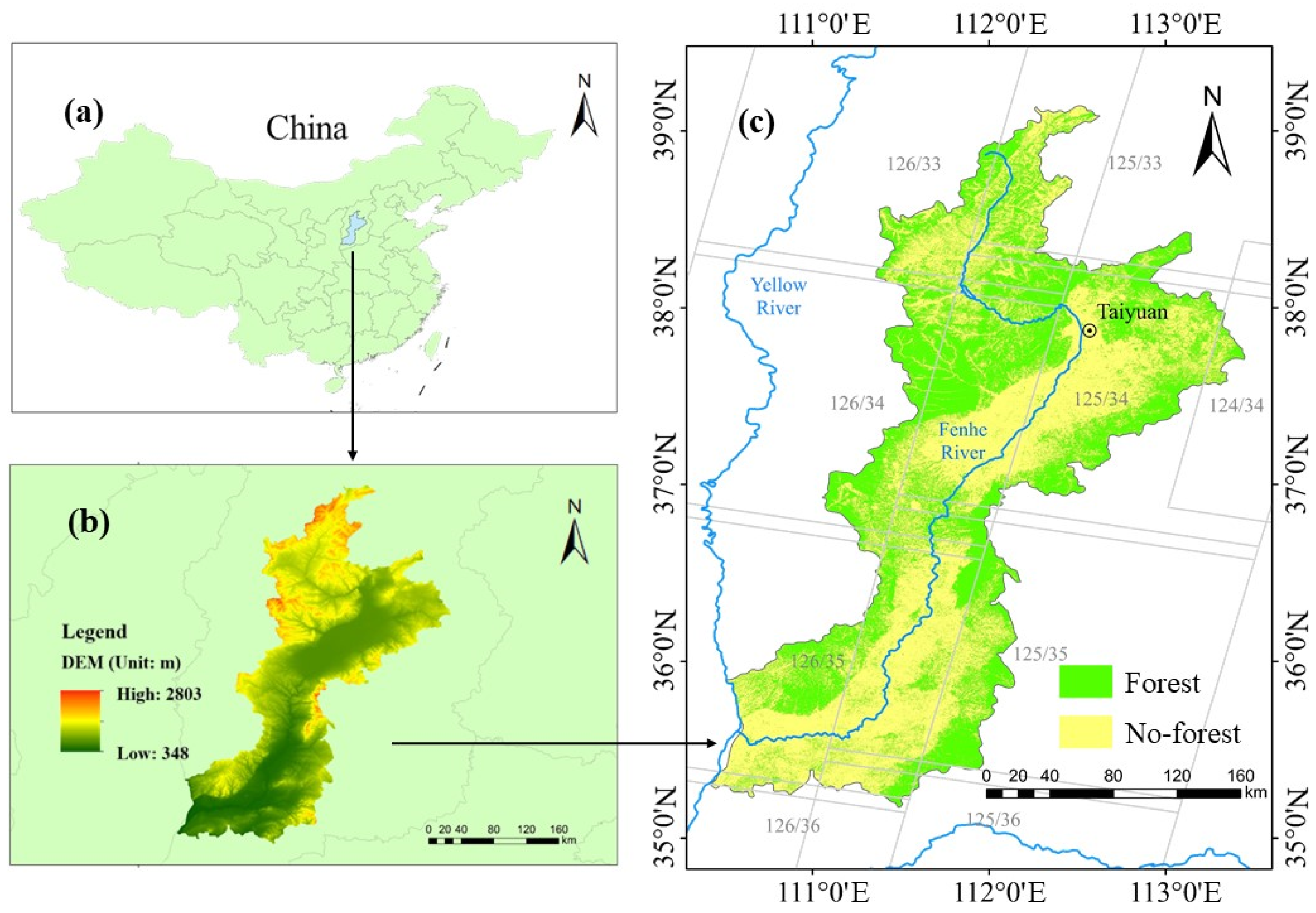
The Fenhe River Basin is located in northern China. Being the second-largest tribu-tary of the Yellow River, the mainstream of the Fenhe River system is 713 km in length, with a basin area of 39,721 km2. It traverses across six cities: Xinzhou, Taiyuan, Jinzhong, Luliang, Linfen, and Yuncheng, and 45 counties (cities, districts). The Fenhe River Basin has a temperate continental climate and belongs to an inland semi-arid area. The annual rainfall is 360 to 700 mm, mainly concentrated between June, July, and August. The mean temperature is 4.2 to 14.2 °C [50]. The terrain of the entire Fenhe River Basin is high in the north and low in the south (Figure 1b). Additionally, the middle zone of the Fenhe River Basin is covered by loess soil (with uneven thickness, undulation, and crisscross ravines), which is a typical landform of the Loess Plateau, and has experienced serious soil and water loss. The Fenhe River Basin is one of the largest coal production zones of China [51]. Mining-related activities have damaged the ecological environment, such as causing forest degradation that is difficult to recovery [52]. Therefore, the government has adopted a series of ecological restoration projects to increase forest coverage. A large amount of agricultural land was converted into economic forest. In the past 30 years, the forest landscape pattern of the Fenhe River Basin has changed frequently with social and natural development [7].
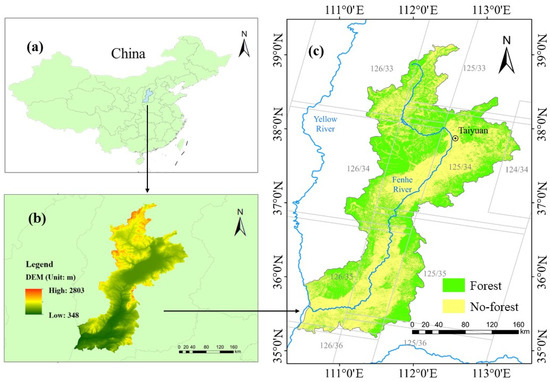
Figure 1.
Location of the study area: (a) general location in China; (b) digital elevation model (DEM) of the study area; and (c) forest area of Fenhe River Basin in 2020.
2.2. Methods
2.2.1. Methodology
The framework of the research method used in this study is shown in Figure 2. First, landscape metrics were calculated according to the land cover map obtained by a random forest classifier on the Google Earth Engine (GEE) platform. Second, the four landscape indices were used to identify the three spatial heterogeneous patterns using the Self Organizing Maps (SOM)+K-means two-stage classification method, and the time series was constructed. Then, the operation rules of frequent sequence pattern mining were defined, frequent sequence patterns under different parameters were mined, and their spatiotemporal variation characteristics were analyzed. “Landscape stability” refers to the ability of a landscape to maintain its states and quickly recover after being disturbed by external forces [53]. By referring to a report by Mukherjee et al. [28], this study defines “landscape stability” from the spatial perspective as the weaker forest landscape stability with greater fragmentation as well as the stronger forest landscape stability with less fragmentation. From the time-scale perspective, the stability of forest landscapes with a high frequency of disturbance and recovery events is weaker, but the stability of those with a low disturbance and recovery frequency is stronger. Finally, based on the types of landscape patterns in the spatial scale and the frequent sequence patterns in the temporal scale, this study evaluates the stability of the forest landscape patterns in the Fenhe River Basin.
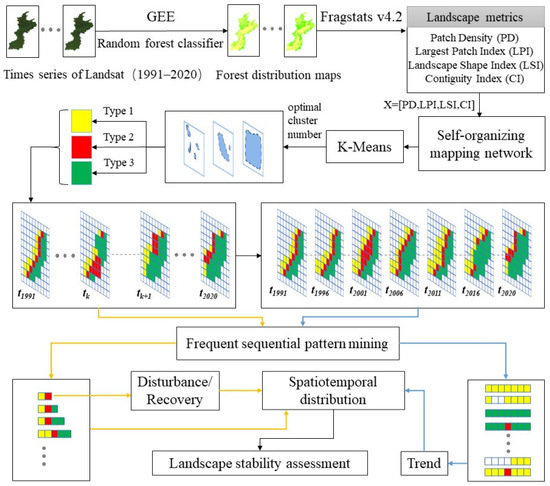
Figure 2.
Schematic representation of the framework of the research method applied in this study; Google Earth Engine, GEE.
2.2.2. Data Preparation
The GEE is a free data cloud platform that can be used for planetary scale analysis (https://earthengine.google.org/ (accessed on 25 March 2021)). Radiation correction with high accuracy was performed on the surface reflectance of the Landsat data archived on the platform. Atmospheric correction eliminated the atmospheric effects due to absorption and scattering. Terrain processing of level 1 accuracy was also performed. We downloaded the annual L1T Landsat remote sensing images of WRS-II numbered 124/34, 125/33–36, and 126/33–36 (Figure 1c) from 1991 to 2020 on the GEE platform. Landsat-5 TM images from 1991–2000 and 2003–2011 were selected as supplements to reduce the impact of SLC-off gaps on Landsat-7 images. Landsat-7 ETM+ images from 2001 to 2002, 2012 and Landsat-8 OLI from 2013 to 2020 were also selected. To reduce the impact of phenological factors, images of the cutting period were selected from June to September for each year. The image quality was controlled by removing all pixels marked as clouds, shadows, or snow from the BQA (Quality Assessment Band) of the satellite images. Finally, the median value of the annual image collection was selected to obtain the annual image. The number of remote sensing image scenes used per year is shown in Table 1. The auxiliary data included the NASA Digital Elevation Model (NASADEM) and high-resolution historical images from Google. The download and processing of all Landsat data and digital elevation models (DEMs) were performed on the GEE platform.

Table 1.
The number of remote sensing image scenes in different years used in this study.
The forest distribution map is the basic data used to calculate the landscape index. The land cover types in the study area were divided into six categories: forest, water, cultivated land, construction land, grassland, and unused land [32,54]. This study defined the Fenhe River Basin forest as land area having a canopy density >30% [32]. The random forest classifier [55] encapsulated on the GEE platform was used to generate land cover maps from 1991 to 2020. All the bands of the Landsat images were input into a random forest classifier for prediction and training samples by visual interpretation based on Landsat images. Approximately 1000 points were marked each year, of which at least 500 were forest samples, and the remaining sample data were used to classify other land cover types. The accuracy of the classification was evaluated using the overall accuracy and kappa coefficient. The accurate criteria of the classification data were that the overall accuracy was >90%, and the Kappa coefficient was >85%. Finally, the forest mask corresponding to the land cover map from 1991 to 2020 was selected as the study area.
2.2.3. Calculating Forest Landscape Metrics
As the calculation of many landscape metrics is based on various statistical processing of patch circumference and area, redundancy is inevitable [56]. We selected four landscape metrics with less correlation: patch density (PD), largest patch index (LPI), landscape shape index (LSI), and contiguity index (CI). These four metrics can be referred to as the “FRAGSTATS Help” [57]. To select an appropriate spatial scale for the forest landscape pattern, we calculated the scale variance of patch density (from 11 × 11 pixels to 111 × 111 pixels (10 pixels between each scale)) and each pixel (with a grid cell size of 30 m × 30 m) [58,59,60]. The smallest scale variance was obtained from 21 × 21 pixels. Therefore, in this study, 21 × 21 pixels was the most appropriate grid cell size. FRAGSTATS 4.2 is a software that quantitatively analyzes landscape structure composition and spatial pattern and can calculate hundreds of landscape metrics [57]. We calculated four landscape metrics using the software; in total, 95712 effective grid cells were calculated.
2.2.4. Extracting Landscape Pattern Types
SOM can reveal the potential distribution patterns and relationships among multiple variables and transform the complex nonlinear statistical relationships between high-dimensional data into simple geometric relationships and show them in a low-dimensional manner [61]. Therefore, we used SOM, which has been proven effective in extracting landscape pattern types in earlier studies [29,62]. Four landscape metrics (PD, LPI, LSI, and CI) were used as input data to construct a feature vector of x = [PD, LPI, LSI, CI]. Notably, the output layer of the SOM calculates the minimum distance of the feature vector, finds the rules, and classifies them. The SOM algorithm references the SOMPY library in Python (https://github.com/sevamoo/SOMPY (accessed on 25 March 2021)), and the SOM algorithm conducts preliminary clustering of massive sample data; feature vectors having similar features are classified into one category. Based on this, the output results of the SOM are taken as the input of the K-means algorithm for further clustering. In this study, the Davies–Bouldin index (DBI) was selected to evaluate the effect of clustering [62]. We selected the optimal cluster number by considering the minimum similarity and maximum heterogeneity within and between the regions, respectively [29,30]. In our study, different labels were assigned to landscape types according to the degree of fragmentation. Notably, we found that landscape fragmentation and the stability of the landscape are inversely proportional to each other [28].
2.2.5. Extracting Frequent Sequential Pattern
Frequent sequential pattern mining refers to the process of finding frequent subsequences (as patterns) from a time-series dataset composed of multiple time series [45]. Furthermore, a candidate set composed of different subsequences is generated, wherein each sequence is ordered by repeatable labels (the landscape pattern type in this study). When a threshold of the occurrence frequency of a subsequence is given, all subsequences that exceed this threshold are called frequent sequence patterns. In this study, we used frequent sequence patterns to identify the temporal relationship between landscape pattern types.
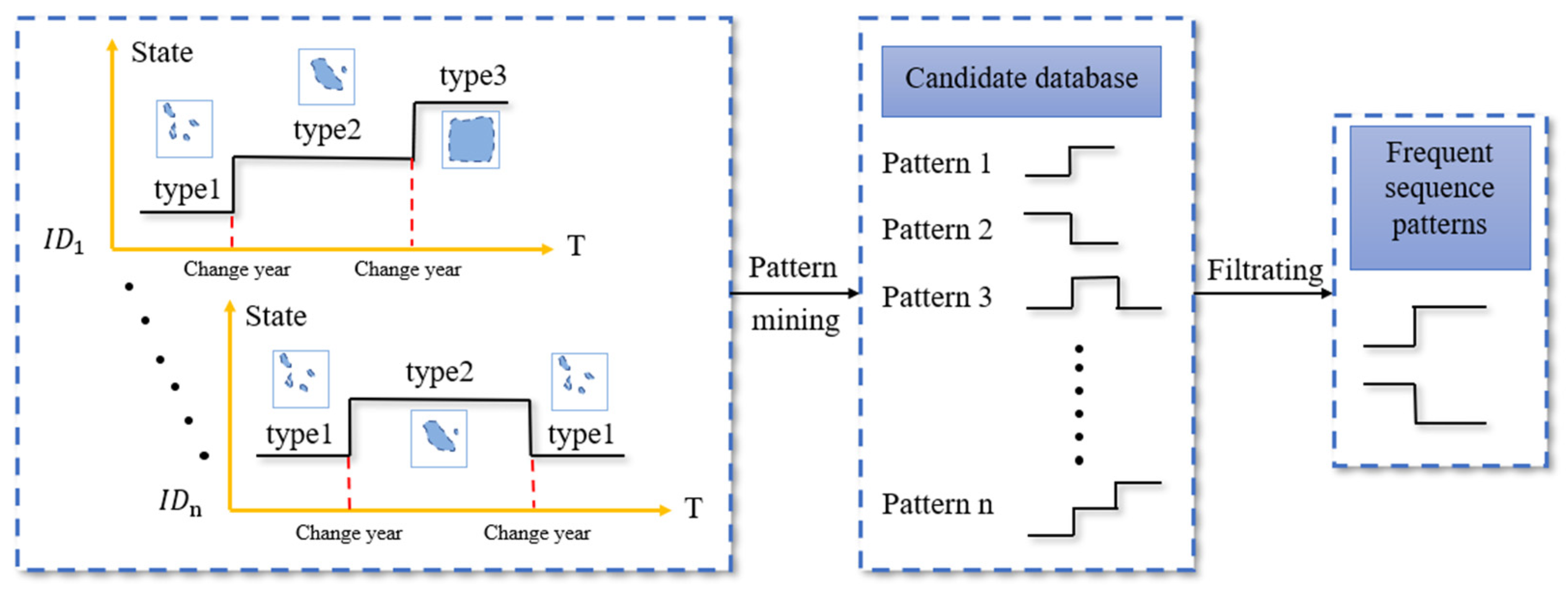
Before data mining, we built a dataset of n time series based on the landscape pattern types data. Frequent sequential pattern mining is divided into two processes: the first step is to generate a candidate database, and the second step is filtration (Figure 3). First, we used the sliding window method to mine the candidate sequence patterns (subsequences). The sliding window is a time window model for common data pattern mining. In this method, the old data are eliminated as the new data enters the window; thus, the internal data of the window are constantly changing. Based on the landscape pattern data set of this study, a sliding window traversed each time series in the data matrix, by automatically adjusting the size of the sliding window. Therefore, each time the window slid, its window sequence formed a candidate pattern. By constantly changing the sliding window size from 1 to 30, all sequence patterns of different lengths were stored to generate a set of candidate sequences. Then, we counted the frequency of candidate sequences, calculated the relative support (Formula (1)) and confidence (Formula (2)) of each sequence pattern, and filtered the patterns that were greater than the minimum relative support () and minimum confidence (β) thresholds. These sequential patterns were classified as frequent sequential patterns and are considered more valuable than other patterns.
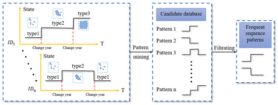
Figure 3.
Schematic of frequent sequential pattern mining. ID is the location of the landscape cell; “T” is the year; “type” is the type of landscape pattern; and “Pattern” is sequence pattern classes.
The support parameter represents the number of occurrences of sequential patterns in the candidate database. If the number of subsequences = <,,……,> in the candidate database is m, and m is called support, which is recorded as , then, relative support is defined as the ratio of the number of to the total number of subsequences. We used to denote the total number of subsequences in the candidate database. The relative support was recorded as . For sequential pattern , the degree of support can be expressed mathematically as follows:
The confidence parameter is defined as the ratio of to , which is recorded as . Here, = <,,……,> and = <,,……, >. The formula is as follows:
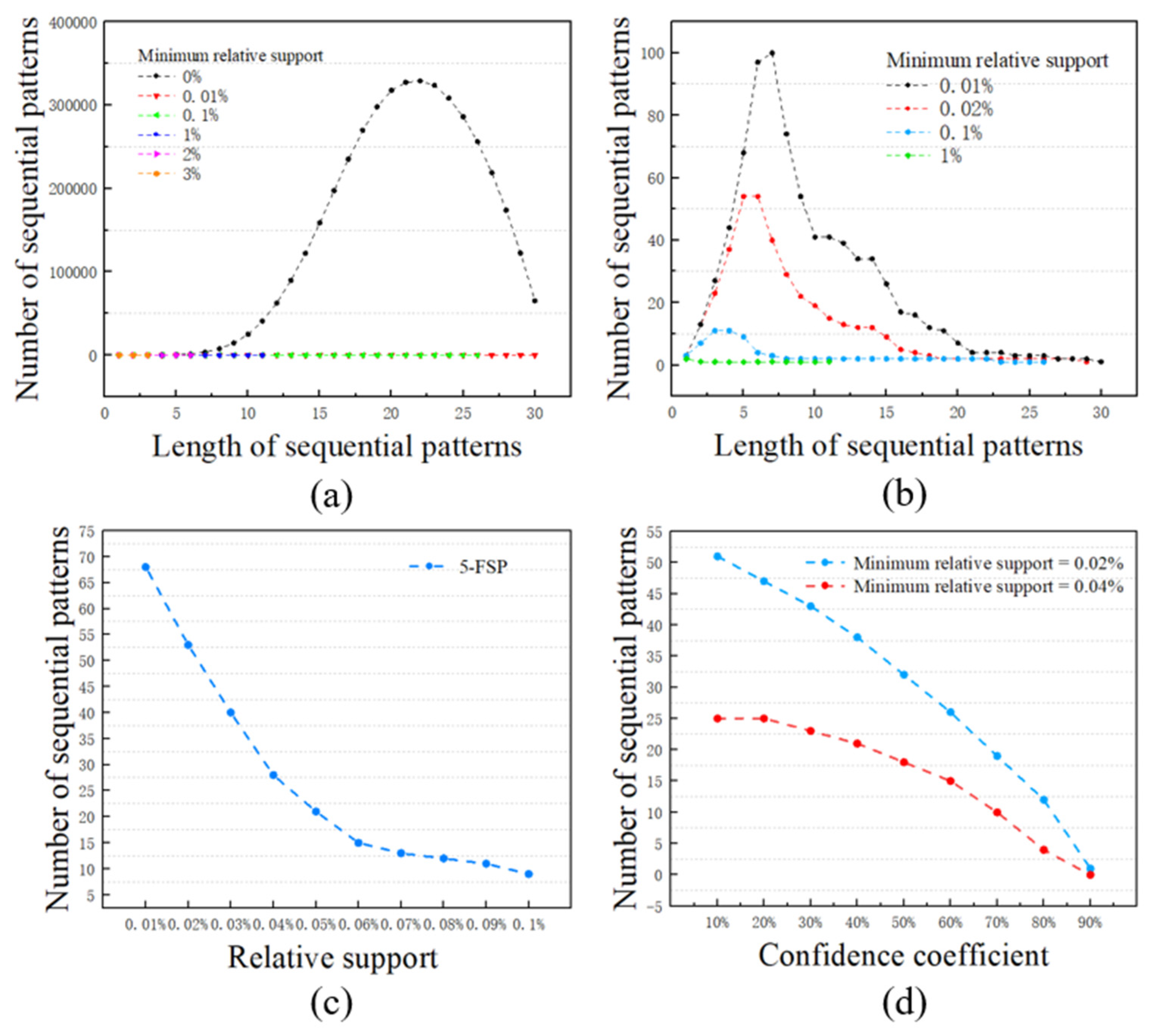
The user specifies the minimum relative support and minimum confidence threshold. The principle of specifying a threshold is: the higher the threshold, the fewer patterns the algorithm generates, and lowering the threshold increases the number of patterns (Figure 4c,d). When is certain for a dataset, the minimum confidence can be eliminated. To ensure the number of patterns generated and the effectiveness of this method, we used a strategy of repeated experiments to determine the threshold. Frequent sequential patterns (FSPs) of length “n” were recorded as “n-FSP”. Assuming that A and B, respectively, represent the type of landscape pattern. Each frequent sequence pattern in the sequence set is expressed by a label, for example, “AAABB” represents the frequent sequence pattern “A→A→A→B→B”. All the programs were implemented in Python.
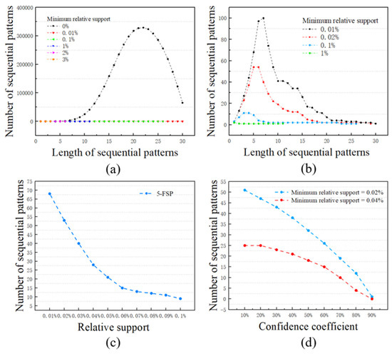
Figure 4.
Plots depicting the relationship between different parameters and the number of frequent sequential patterns. (a) The relationship between the length of the sequence patterns and the number of sequence patterns with minimum relative support under [0, 3%], (b) relationship between the length of the sequence patterns and the number of sequence patterns with minimum relative support under [0.01%, 1%], (c) relationship between relative support and the number of 5-FSP, and (d) relationship between confidence and the number of frequent sequential patterns.
Spatiotemporal Distribution of Typical Frequent Sequential Patterns
First, we mined frequent sequential patterns based on the time series of annual images. We tested the relationship between different parameters (the length of frequent sequential patterns, minimum relative support and minimum confidence threshold) and the number of frequent sequence patterns, as shown in Figure 4. Second, to analyze the spatiotemporal distribution of forest landscape pattern evolution, the following indicators were used to evaluate typical frequent sequence patterns: (1) frequency of pattern in the same area; (2) first occurrence time of the pattern; and (3) the proportion of the area that appears every year, that is, the ratio of the landscape cell area covered by the sequence pattern to the total forest landscape cell area.
Short Patterns about Fragmentation and De-Fragmentation
Each change in landscape pattern type is called an “event”, and these changes were also observed in 2-FSP. These short patterns offer general information about fragmentation and de-fragmentation. Thus, after excluding stable 2-FSP, we categorized other 2-FSPs as fragmentation and de-fragmentation patterns. To reduce the missed detection rate, we set the relative support and confidence to 0. The fragmented and de-fragmented 2-FSPs were defined as disturbance and recovery events, respectively. The number and time of occurrence of the fragmentation and de-fragmentation events in the time series were recorded, and the area proportion of their occurrences each year was counted.
2.2.6. Long-Term Evolution Process and Trend of Forest Landscape Pattern
Due to the significant differences in the geographical location, development stage, and artificial or natural disturbance of the forests in the Fenhe River Basin, there may be potential differences in the forest evolution processes and distribution characteristics. Because there may be many potential sequential patterns in the 30-year-long time series that the coverage area of each pattern is very small, it is not conducive to interpretation and visualization. Thus, we used the method of selecting time intervals of four or five years, reconstructed the time series from the data of 1991, 1996, 2001, 2006, 2011, 2016, and 2020, and extracted the frequent sequence patterns. Further, 7-FSP values larger than the minimum support and minimum confidence were visualized. Notably, the direction of landscape change summarized the historical trends of change and reflected the differences in different periods. According to the fragmentation trend, the long-term evolution process was defined as fragmentation, de-fragmentation, stability, and fluctuation.
3. Results
3.1. Spatial Characteristics and Interannual Trends of Different Landscape Pattern Types
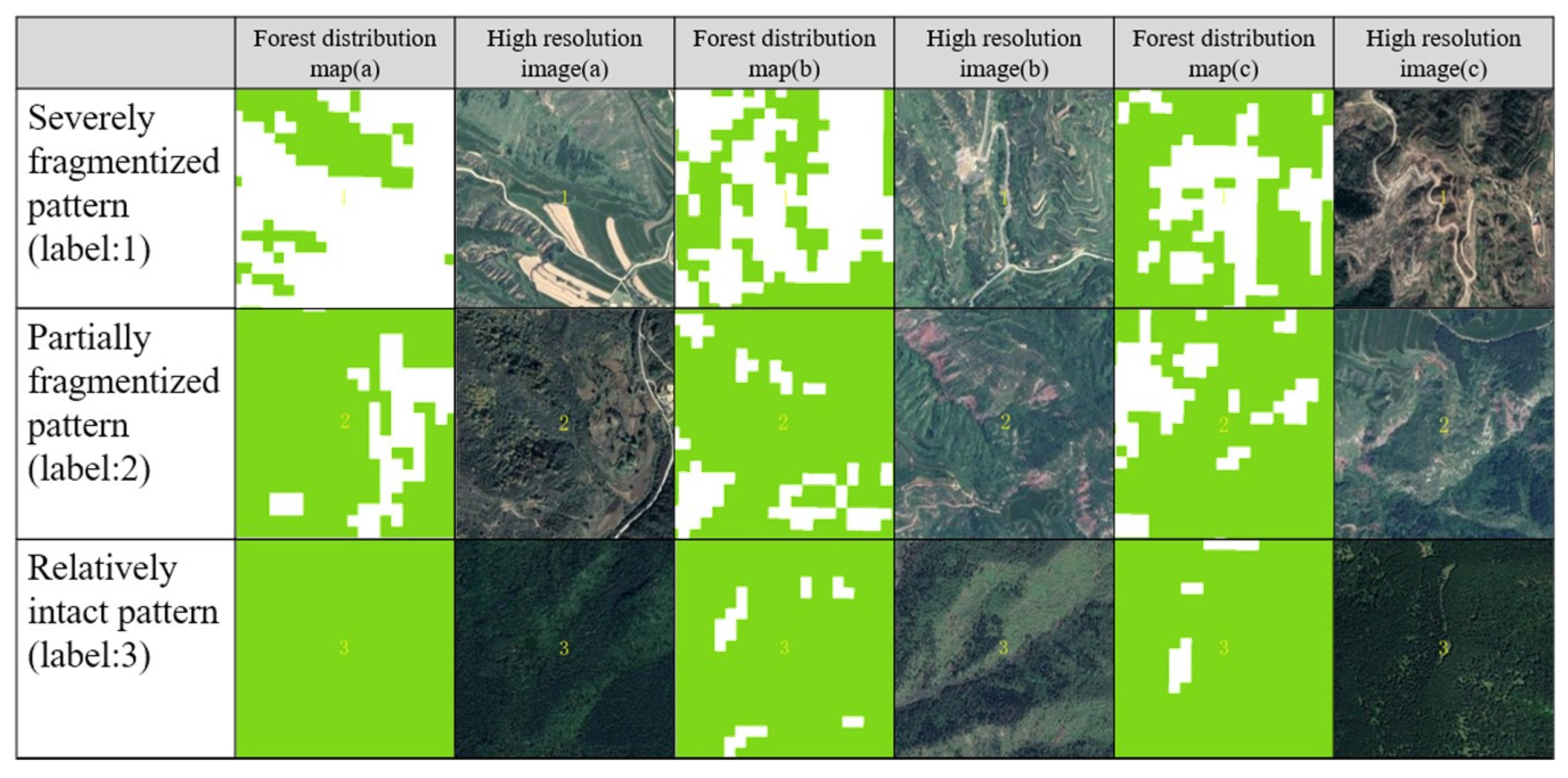
First, we used DBI to test the effect of k-means clustering, and the range of the number of clusters was 3–9. According to the minimum value of the DBI for different cluster numbers, we chose the optimal cluster number as 3 (Table 2). Second, landscape cells that are severely fragmented are labeled 1, partially fragmented are labeled 2, relatively complete are labeled 3, and non-forest are labeled 0. Figure 5 shows a comparison of forest landscape cells and high-resolution images from June to September 2020 with different labels. Third, we constructed a collection of time series, based on the labels of these landscape pattern types.
Table 2.
Performance of Davies–Bouldin index (DBI) in different cluster numbers.

Figure 5.
Tabular depiction of the comparison of forest landscape cells and high-resolution images with different labels (a, b, and c of each category for the same landscape cell).
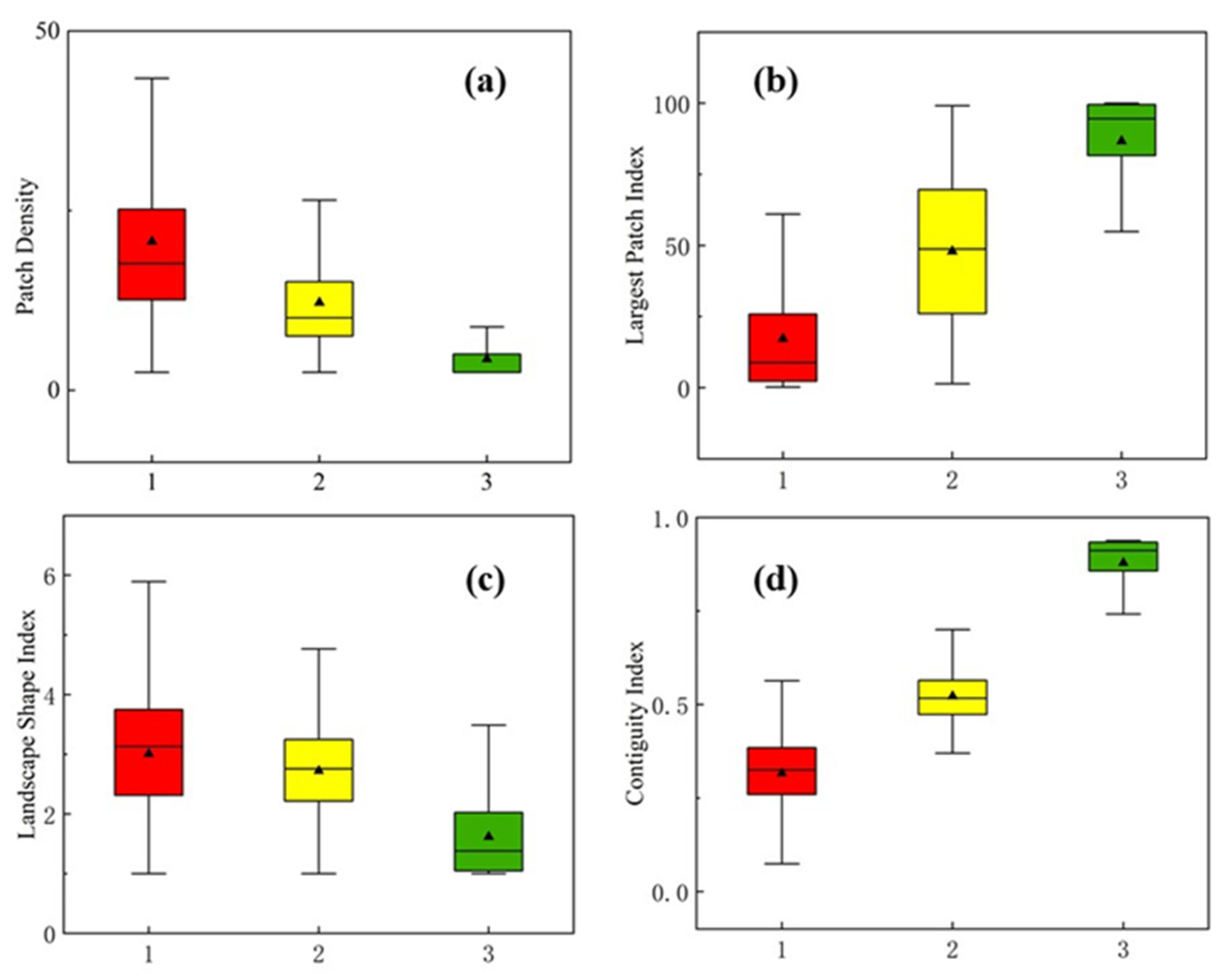
We observed the spatial characteristics and inter-annual trends of different landscape pattern types. As shown in Figure 6, according to each index of landscape in the three types of landscape patterns of the distribution, the severely fragmentized pattern had a larger PD and LSI and a smaller LPI and CI. This indicates that this type of forest landscape cell contains multiple scrawled forest patches, and patches of boundary shape are complicated, or patches with larger internal perforations. Generally, the forest area takes up less of the landscape cell. The average value of each landscape metric in the partially fragmented pattern was between a severely fragmented and a relatively complete pattern, and this category is primarily composed of large patches mixed with small patches. The relatively complete pattern had a larger LPI and CI and a smaller PD and LSI. The forest patches they contained were relatively complete, and almost all of them were covered by forests. As shown in Figure 7, the annual area of the landscape cell category (from 1991 to 2020) was determined.

Figure 6.
Plots showing the distribution of forest landscape metrics: (a) patch density (PD), (b) largest patch index (LPI), (c) landscape shape index (LSI), and (d) contiguity index (CI). (Label 1: severely fragmentized pattern, Label 2: partially fragmented pattern, Label 3: relatively complete pattern).
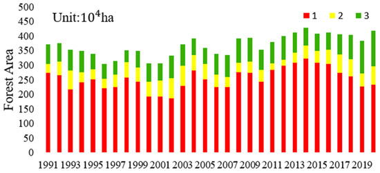
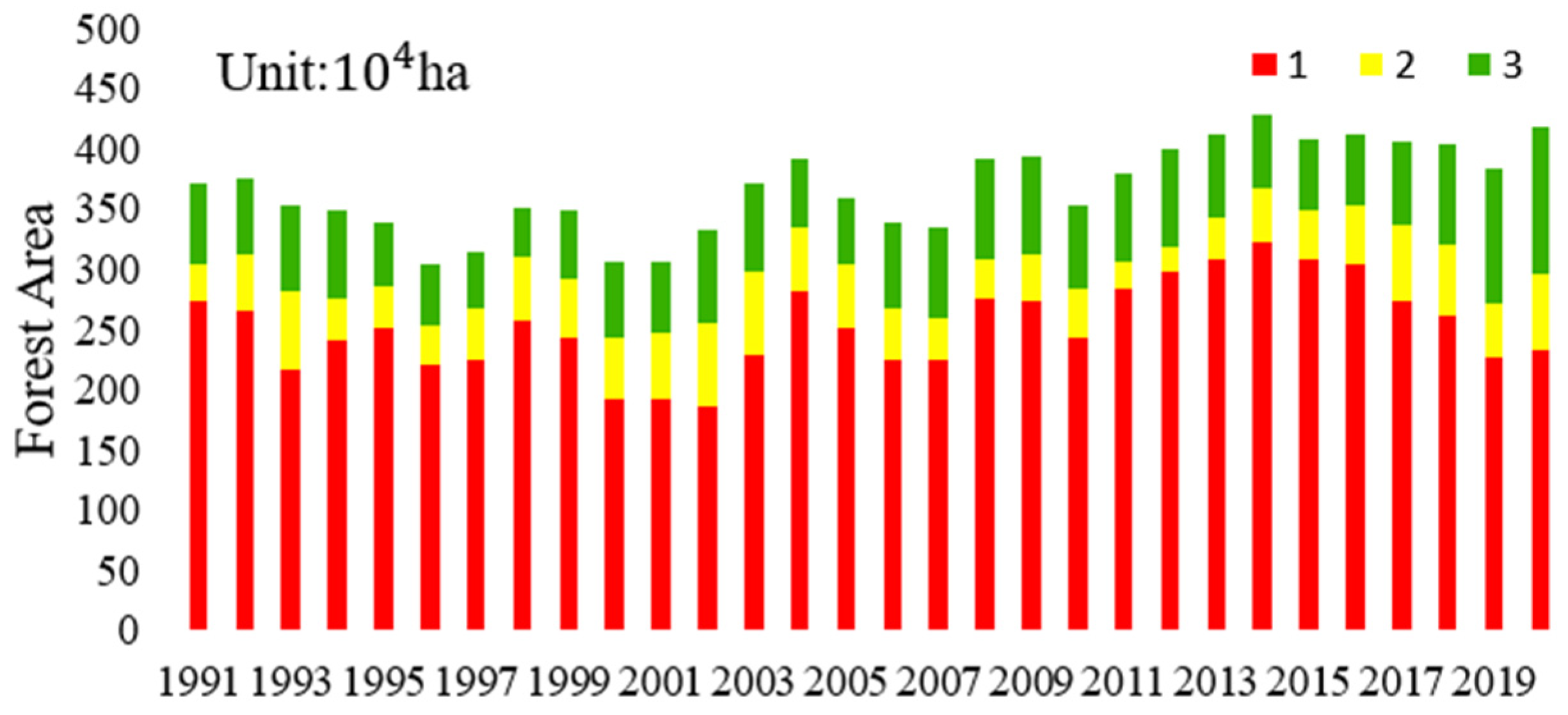
Figure 7.
Graphical representation of the area changes of forest landscape pattern types from 1991 to 2020.
3.2. Extracting Frequent Sequential Pattern
3.2.1. Spatiotemporal Distribution of Typical Frequent Sequential Patterns
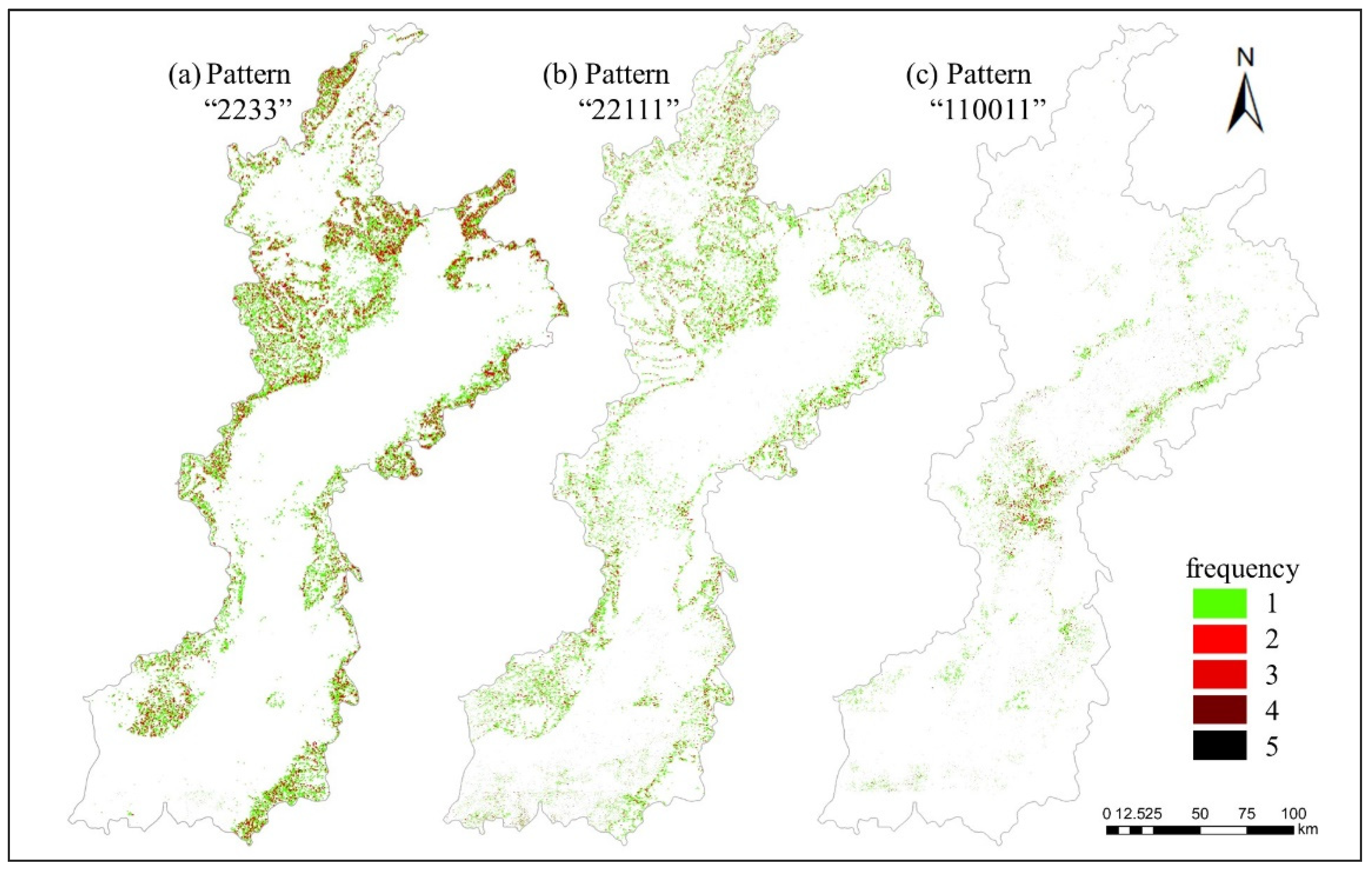
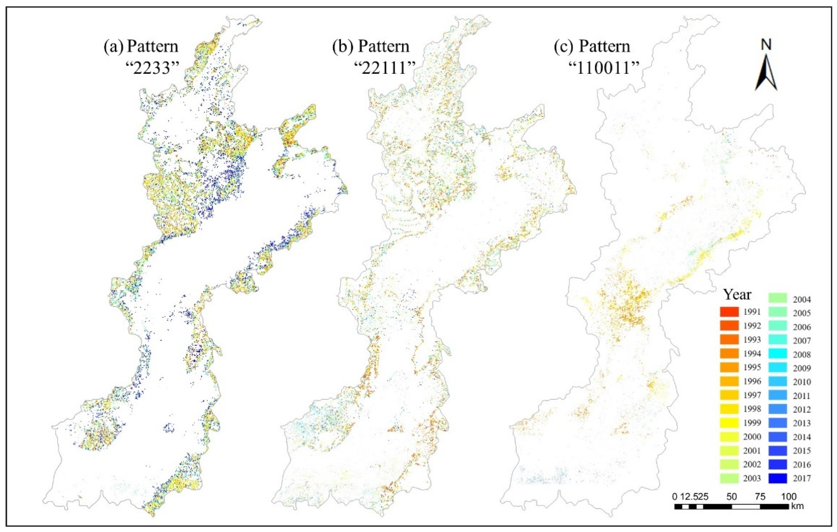
Under the constraint of minimum relative support and minimum confidence of 0.03% and 60%, respectively, we obtained 218 sequential patterns. We considered the sequential patterns “2233”, “22111”, and “110011” as examples because they correspond to the three most common and typical trends in the process of forest change. The relative support and confidence of pattern “2233” were 0.06% and 94.72%, respectively. The relative support and confidence of pattern “22111” were 0.06% and 82.78%, respectively. The relative support and confidence of pattern “110011” were 0.036% and 73.71%, respectively. Generally, the sequence patterns of the downward trend accounted for a small proportion. Notably, the fluctuant trend had the largest number of sequential patterns, and the relative support of each fluctuating sequential pattern was very small.
The pattern “2233” represents that the forest landscape pattern has changed from a partial fragmentation pattern to a relatively complete pattern in the third year, indicating that the local forest has become lush during this period, indicating forest restoration. This pattern has a large number of sequence patterns with time and a large coverage area (Figure 8a). The pattern “22111” changed from a partial to a serious fragmentation pattern in the third year, indicating forest degradation. The most frequent occurrence of this pattern was on the edge of the forest and near the road (Figure 8b). Pattern “110011” indicates that the level of the landscape pattern of forest decreased during a certain period, although the level returned to a seriously fragmented pattern in the fifth year. The pattern is primarily distributed in the middle of the Fenhe River Basin and the forest edge (Figure 8c).
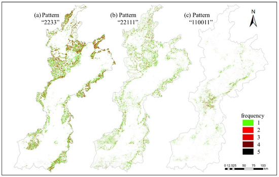
Figure 8.
Spatial gradient map depicting the frequency distribution of frequent sequential patterns: (a) pattern “2233”; (b) pattern “22111”; and (c) pattern “110011”.
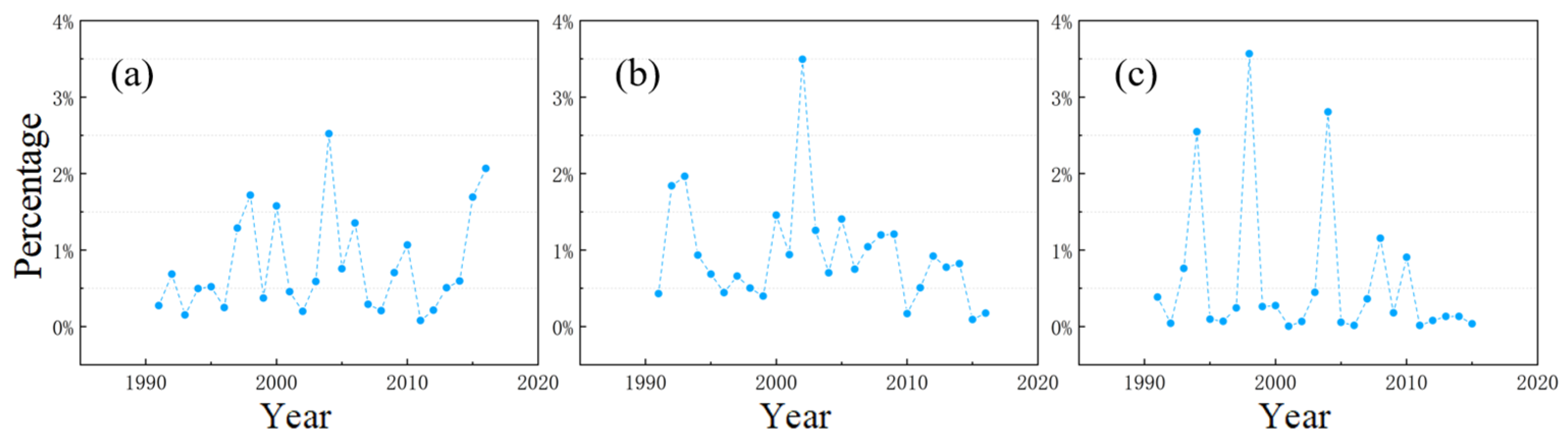
The pattern “2233” showed a maximum of 2.52% in 2004, with an annual increase till 2011 (Figure 9a). The year with the highest frequency of the pattern “22111” was 2002, resulting from 3.49% (Figure 9b). The proportion of pattern “110011” was less in most years (Especially in 2010) and more in 1994, 1998, and 2004 (Figure 9c).
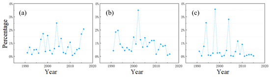
Figure 9.
Plots showing the change of area proportion of frequent sequence patterns with time: (a) pattern “2233”; (b) pattern “22111”; and (c) pattern “110011”.
In 1991, pattern “2233” first appeared within the forest region and then, at the edge of the forest (Figure 10a). This indicates that the forest stability has improved during a certain period, and the process of improvement first occurred in the core area of the forest and then, at the edge of the forest. Pattern “22111” shows that forest stability declined during a certain period, most of which occurred before 2000 (Figure 10b). Pattern “110011” shows that the forest stability decreased first and then, increased in a period; for the first time, the pattern mostly occurred before 2000 (Figure 10c).
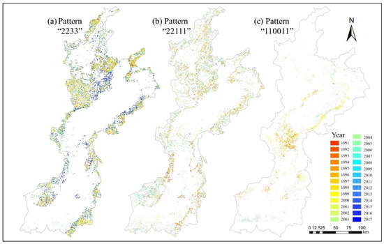
Figure 10.
Gradient overlay map depicting spatial distribution of frequent sequential patterns that appeared for the first time: (a) pattern “2233”; (b) pattern “22111”; and (c) pattern “110011”.
3.2.2. Short Patterns about Fragmentation and De-Fragmentation
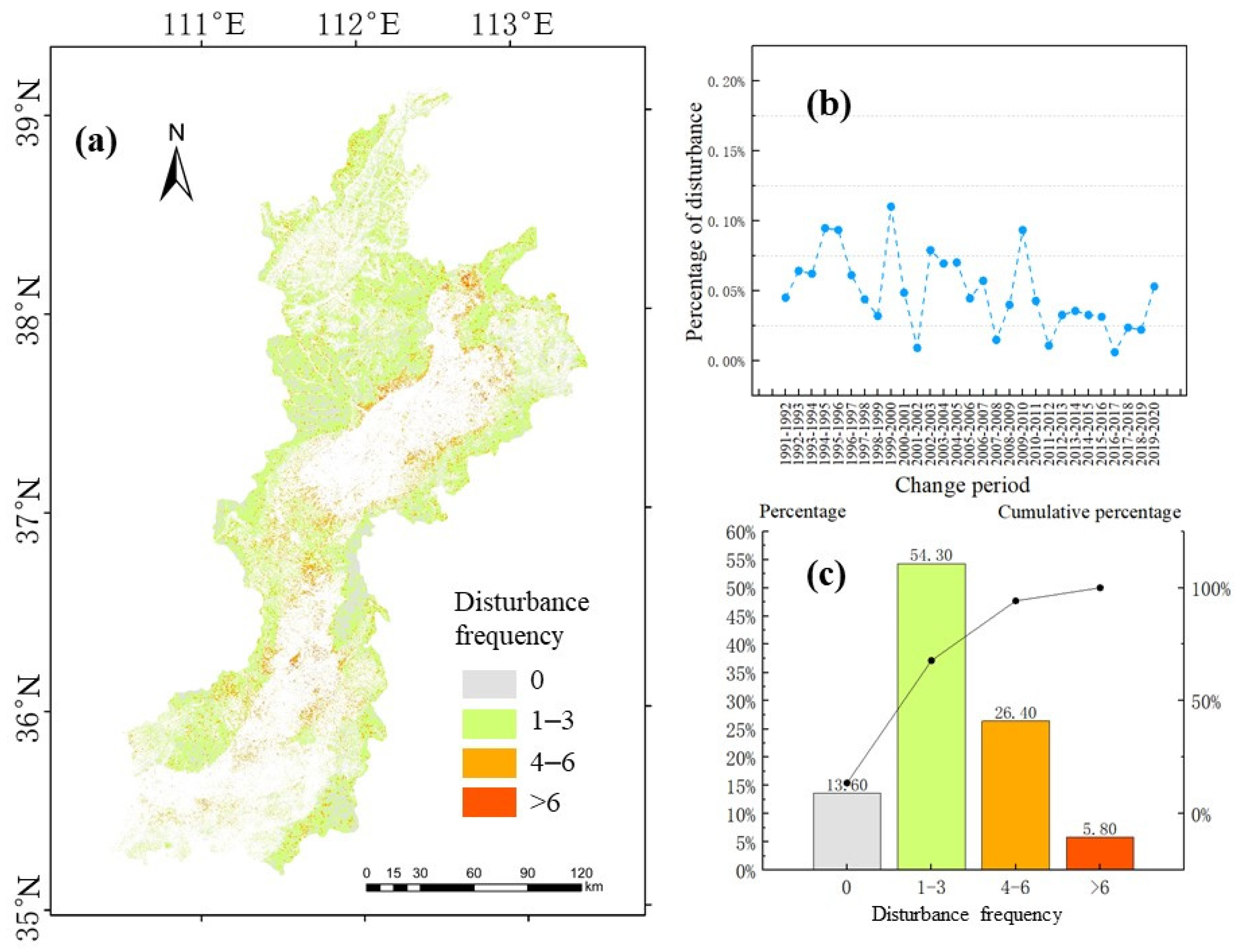
As shown in Figure 11a, the places with more disturbance frequency are primarily distributed in the border area between the forest and non-forest areas and in the middle of the Fenhe River basin. With respect to time, as shown in Figure 11b, the largest area of disturbance occurred during 1991–2000 (0.11%) and the smallest was during 2016–2017 (0.005%). Overall, the proportion of disturbed forests showed a downward trend from 1991 to 2020. From a spatial perspective, as shown in Figure 11c, the ratio of 1–3 times was the highest (54.3%), and that of more than 6 times was the lowest (5.8%).
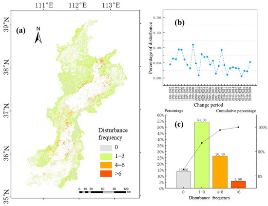
Figure 11.
Temporary and spatial distribution of forest disturbance events: (a) gradient map of the spatial distribution of disturbance events; (b) plot of the area of the disturbance ratio changes over time; and (c) bar plot depicting the statistics of disturbance frequency.
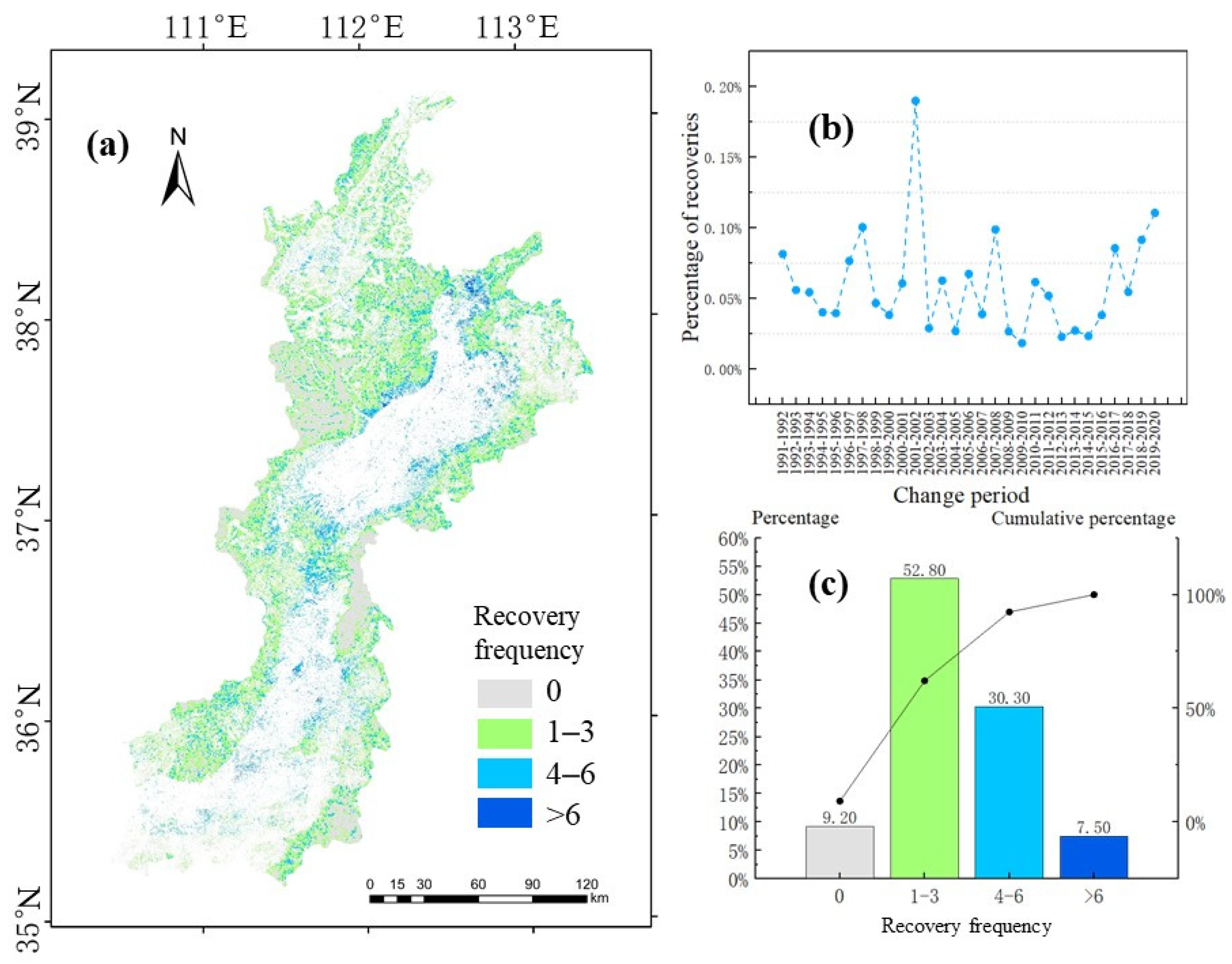
As shown in Figure 12, the places with higher frequency were primarily distributed in the area at the junction of the forest and non-forest areas and in the middle of the Fenhe River Basin. As shown in Figure 12b, there was a sudden increase in the number of recovery events between 2001 and 2002, which accounted for 0.18% of the area; it accounted for 0.018% during 2009–2010. Overall, it fluctuated before 2014 and increased annually since 2014. One of the reasons for the abrupt increase in the area from 2001 to 2002 compared to that of 2000 to 2001 may be that, during the early stage, the original farmland was converted to forests or other economic forests under the promotion of policies that were planted. As shown in Figure 12c, the proportion of 1–3 recoveries were the highest (52.8%), and the lowest was more than 6 times (7.5%).
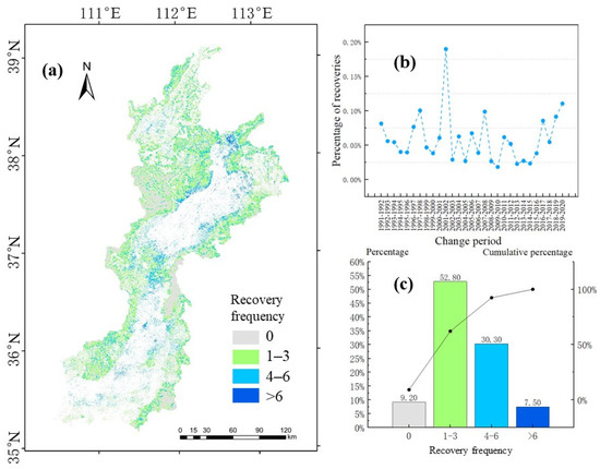
Figure 12.
Temporary and spatial distribution of forest recovery events: (a) gradient map of the spatial distribution of recovery events; (b) plot of the area of the recovery ratio changes over time; and (c) bar graph showing the statistics of recovery event frequency.
In the past 30 years, the total area of forest recovery events was 749 (), which is larger than that of disturbance events of 621 (). The location of the recovery events was similar to that of the disturbance events, and there was a negative correlation with time, with a correlation coefficient of −0.4429.
3.3. Long-Term Evolution Process and Trend of Forest Landscape Pattern
For relative support of 0.10% and confidence of 50%, we obtained ten 7-FSP evolution patterns (Table 3). The distribution map of the pattern is visualized as shown in Figure 13, where different colors are used to distinguish different sequential patterns, which represent the evolutionary trajectory of the landscape pattern. Notably, although all land cover types are forests, the evolutionary history within forests is significantly different. Spatially, the same evolution pattern was gathered. The location was relatively close, which may be due to the same artificial or natural interferences in the same period. Temporally, some patterns showed the transformation from disturbance to restoration. The changes in the fragmentation degree of patterns 1 and 3 were relatively stable, and the elevation of pattern 3 was higher and distributed centrally. Forests in areas covered by patterns 2, 4, 5, and 6 may disappear. Pattern 2 was primarily distributed in the central part of the Fenhe River Basin, and it was observed where terraced fields were widely distributed. Patterns 7 and 8 represented the areas having increased forest coverage.
Table 3.
Ten evolution patterns of forest.
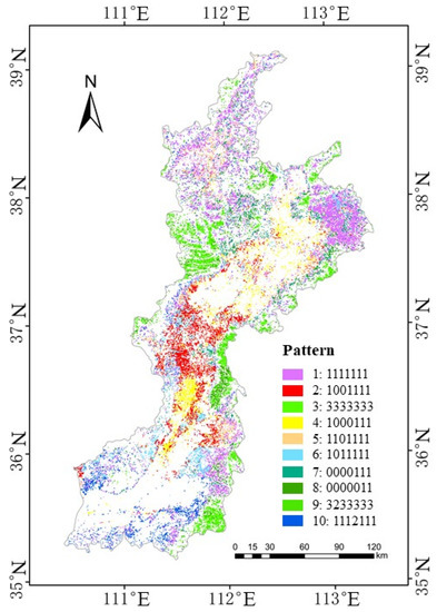
Figure 13.
Spatial gradient map depicting the long-term forest evolution pattern in the Fenhe River Basin.
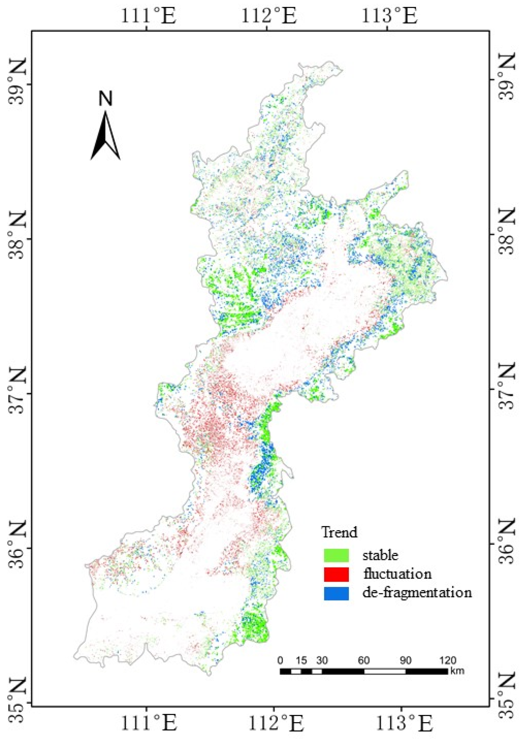
As shown in Figure 14, each color represents an evolutionary trend. The area proportion of the fluctuant pattern was 12.9%, stable pattern was 12.1%, and de-fragmentation pattern was 3.4%. The fluctuating pattern occupied a dominant position in the Fenhe River Basin and was primarily concentrated in the middle of the basin. The local people have developed many terraces in this area, which are also areas with serious soil and water loss. Notably, most of the stable ones are located in areas with higher elevations and less artificial disturbance. Contrastingly, the de-fragmentation regions are scattered in the transitional zone between the forest and non-forest areas.
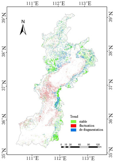
Figure 14.
Spatial gradient map showing the long-term evolution trend of forests in Fenhe River Basin.
4. Discussion
4.1. Value and Applicability of Frequent Sequential Patterns
Landscape analysis aims to not describe the landscape but explain and understand the process [14]. The method proposed in this study can detect rising, falling, stable, and fluctuant frequent sequential patterns at different temporal scales. Sequential patterns can express information in both temporal and spatial dimensions simultaneously, which is difficult for other methods. The sequential pattern can provide scientific support for forest managers to formulate efficient forest management plans. Pattern “110011” may be the area of returning farmland to the forest because the forest may disappear, and it can be used as an area to prevent forest depletion. The pattern “2233” mostly appeared in the core areas within the forest, which can be the areas where the forest ecosystem continues to be optimized. Spatially, similar to the reports of Oikonomakis, Nikolaos, and Petros Ganatsas [63,64], pattern “22111” mostly occurred at the edge of the forest and near the road, and this process may be caused by artificial land-use change, leading to an increase in fragmentation. Temporally, this pattern occurred most frequently in 2002; the transformation of farmland to forests was implemented in this year [65]. The forest area increased rapidly, resulting in a rapid decline in fragmentation. However, many regions reemerged in 2004; this shows that the impact of returning farmland to forests is short-term, and the maintenance capacity of the forest ecosystem covered by the pattern “22111” was poor. Some research of Oikonomakis Nikolaos, and Petros Ganatsas [63,64] has considered the succession process between different tree species and the driving factors behind them. Elevation was regarded as a key driving factor. This study finds that high altitudes affect the evolution of forests because they hinder the fragmentation of forest landscapes. Forests in high-altitude areas maintain relatively complete and large patches with relatively strong landscape connectivity. Although with greater landscape connectivity and higher forest coverage, such areas may have a rich succession process of tree species within a forest. This is worthy of continued research. Therefore, it is a very meaningful effort to detect the succession process of different forest stands from two dimensions of time and space simultaneously by using frequent sequence patterns in the future. This effort can help understand the environment—succession interactions. However, in the loess hilly area in the middle of the Fen River Basin, there are many small and often disappearing patches, because local people have developed the virgin forests into terraces, thus destroying the connectivity of the landscape. In addition, mining activities have also transformed large forest patches into small ones, thus weakening the landscape connectivity of forests. Although the forest coverage has been increased through ecological restoration projects and the forest landscape has become complete, the conversion of farmland into economic forests or artificially planted single stands may deliver certain negative impacts to the ecological environment [66]. All these driving factors affect the succession of forests as well as movements of species between patches.
Jerzy Solon [67] and Lídia S. Bertolo [68] combined fragmentation and important driving factors to analyze landscape changes. Jerzy Solon pointed out that the distance from the traffic route had a significant impact on the landscape structure. They used a comparative analysis method, although they ignored the detailed process between different periods. Our method was able to mine this change process, describing the processes using two dimensions: time and space. In addition, we believe that different drive factors have different effects on the evolution process of the landscape.
Compared with the research of Hermosilla et al. [18]. When considering the overall dynamics of the forest by trend analysis, some instantaneous states are smoothed by “space filtration”, making the dynamics of the entire forest look more stable [43,69]. However, in the history of the evolution of the forest, forest dynamics are not always stable. For example, as shown in Figure 10a, pattern “2233” indicates that the stability is enhanced in a certain period and may be affected by the policy. This process has appeared in the northern part of the Fenhe River Basin after 2000. These staged evolutionary processes show the direction of the forest changes. These typical sequence patterns represent landscape stability within a specific period, which helps to strengthen our understanding of the forest landscape.
Forest disturbance and restoration are usually carried out by detecting breakpoints and deviations in the time series composed of forest functions [70,71]. These detection methods pay attention to the time of disturbance occurrence and the trend of the subsequent recovery. Still, they cannot characterize the whole process of disturbance–recovery in both time and space dimensions simultaneously. Although the landscape pattern change has maintained a stable trend for several years, the forest function may still be disturbed before and after the pattern change. The changes in the forest landscape pattern may fall behind in the forest function. Landscape dynamics cannot completely characterize the evolution of forests. Therefore, there have been some studies on the interaction between forest landscape pattern change and function change recently [18,72,73].
4.2. Evaluation of Landscape Stability
Areas that are disturbed frequently or change rapidly may lead to the extinction of species and affect local biodiversity [72]. As shown in Figure 11a and Figure 12a, the forests in most areas have been disturbed or restored 1–3 times, and the rest periods have kept a constant spatial pattern. This shows that once stable conditions are established, the forest will enter another state and last for several years. More than six times are distributed at the junction of forest and non-forest, which indicates that human activities have a greater driving force on landscape change than nature. We believe that the higher the interference frequency, the more unstable it is. The central area of the Fenhe River basin should also be the key area to prevent soil erosion. We used the proportion of the disturbed area to the total forest landscape area to express the overall stability of the forest in the Fenhe River basin [43,69]. As shown in Figure 11b, the area proportion of disturbance shows a downward trend, which indicates that the stability of the forest landscape in the basin has improved. Although we did not set a threshold to divide the landscape stability, the trend of the area proportion shows that the overall landscape stability of the basin is increasing.
The long-term evolution pattern expresses the difference in forest fragmentation in different periods, which can be used to analyze detailed process information and changes in stability. As shown in Figure 13, patterns 2, 4, 5, 7, and 8 have become landscapes that are severely fragmented forests from the non-forest area in 2001 or after 2001, which is consistent with the fact that China has fully implemented the conversion of farmland to forest to increase forest cover [65]. We take sequence pattern 2 as an example to explain the evolution process. The formation of pattern 2 may be due to excessive deforestation and land development (for construction) in the 1990s, coupled with frequent natural disasters (drought, pests, and diseases), which led to the deterioration of the ecological environment. The forest began to disappear in 1991. Since 2006, forests have reemerged in the area, indicating that local forest cover increased during 2001–2006 and has since been a stable sequence. With the implementation of environmental awareness and policies, forests have been effectively managed. As shown in Figure 14, similar to the report of Jerzy Solon, a specific feature of landscape pattern change is the simultaneous occurrence of numerous and frequently contradictory processes [67]. Although the fluctuation process is dominant, there are still many areas with de-fragmentation processes, which correspond to regions with increased stability. This asymmetrical development process also occurs within the forest, contributing to the comparison of forest landscapes in different regions.
4.3. Research Limitations and Future Work
(1) The frequent sequential pattern mining method is still feasible for detecting other non-forest landscapes and can further explore the pattern changes of different non-forest landscapes.
(2) Although we can adopt measures to reduce errors, such as the SLC-off gaps of Landsat7, there are still challenges in achieving accurate classification in cloudy areas (such as southern China).
(3) Indicators applied to frequent sequence pattern mining are not sufficiently rich. Although Julea et al. [49] detected the spatiotemporal changes in crop species, Normalized Difference Vegetation Index (NDVI), and subsidence/uplift movements related to water level fluctuations on the soil surface, other quantitative indicators or qualitative states are rarely combined with frequent sequential pattern mining methods. Therefore, further research can combine more quantitative indicators and states by exploring the evolution of forests.
(4) The evolution of landscape patterns is the result of the joint action of nature and society. It is necessary to determine the role of different driving factors in landscape change and establish a pattern-ecological process model. Therefore, future research can combine the driving factors (such as fire and logging) to construct time series to analyze the spatiotemporal association rules between driving forces and different indicators, for example, the spatiotemporal correlation between indicators and fire, precipitation, and logging. Mining these frequent event combinations <indicators, drivers> and their sequence patterns are particularly important for understanding the impact of ecological processes on the pattern or function.
5. Conclusions
In this study, we proposed a new method for detecting dynamic changes in landscape patterns. The temporal and spatial dimensions were considered to describe the evolution of forest landscape patterns simultaneously. Experiments were conducted in the Fenhe River Basin. Furthermore, we evaluated the landscape stability of forests in this area. The findings and conclusions drawn from this study can be summarized as follows.
(1) The frequent sequential pattern mining method is effective in mining the secondary evolution processes that frequently occur in the dynamics of landscape patterns. Short-term sequential patterns can describe the process of disturbance, recovery, or interference recovery. Furthermore, long-term evolution patterns can describe the trend of forest evolution, state in the process, and landscape stability, which is difficult for other methods to mine simultaneously. The spatiotemporal distribution of sequential patterns is quite different, and its distribution characteristics are helpful for forest managers to design policies related to land degradation and potential environmental pressures.
(2) In the last 30 years, the total area of disturbed forest is less than the total area of forest recovery. There is a negative correlation between the extent of disturbance and recovery events every year, and the proportion of the disturbed regions show a downward trend overall.
(3) A variety of processes occur simultaneously in the same forest ecosystem. According to the evolution process of forest landscape patterns from 1991 to 2020, the same long-term evolution process is mostly aggregated, and the spatial position is relatively close.
(4) Generally, forest stability in the Fenhe River Basin has improved. Relatively complete forest landscape cells have better stability, although they account for a relatively small proportion. Since 2016, its proportion has increased, i.e., more forest landscapes have become complete and stable.
Author Contributions
Conceptualization, X.L. and Y.Z.; methodology, Y.L. and Y.Z.; validation, X.L., Y.Z. and Q.Y.; writing—original draft preparation, Y.Z. and Z.L.; visualization, Y.Z.; supervision, X.L. All authors have read and agreed to the published version of the manuscript.
Funding
This research was funded by the National Natural Science Foundation of China, grant number 41871223.
Acknowledgments
The authors would like to thank the anonymous reviewers and the editor for their constructive.
Conflicts of Interest
The authors declare no conflict of interest.
References
- Baskent, E.Z. Controlling spatial structure of forested landscapes: A case study towards landscape management. Landsc. Ecol. 1999, 14, 83–97. [Google Scholar] [CrossRef]
- Foley, J.A.; DeFries, R.; Asner, G.; Barford, C.; Bonan, G.; Carpenter, S.R.; Chapin, F.S.; Coe, M.; Daily, G.C.; Gibbs, H.K.; et al. Global Consequences of Land Use. Science 2005, 309, 570–574. [Google Scholar] [CrossRef] [Green Version]
- Aragón, R.; Oesterheld, M.; Irisarri, G.; Texeira, M. Stability of ecosystem functioning and diversity of grasslands at the landscape scale. Landsc. Ecol. 2011, 26, 1011–1022. [Google Scholar] [CrossRef]
- Hess, G.R.; Koch, F.H.; Rubino, M.J.; Eschelbach, K.A.; Drew, C.A.; Favreau, J.M. Comparing the potential effectiveness of conservation planning approaches in central North Carolina, USA. Biol. Conserv. 2005, 128, 358–368. [Google Scholar] [CrossRef]
- Zhang, M.; Wang, J.; Li, S. Tempo-spatial changes and main anthropogenic influence factors of vegetation fractional coverage in a large-scale opencast coal mine area from 1992 to 2015. J. Clean. Prod. 2019, 232, 940–952. [Google Scholar] [CrossRef]
- Yan, D.; Bai, Z.; Liu, X. Heavy-Metal Pollution Characteristics and Influencing Factors in Agricultural Soils: Evidence from Shuozhou City, Shanxi Province, China. Sustainability 2020, 12, 1907. [Google Scholar] [CrossRef] [Green Version]
- Cao, Y.; Bai, Z.; Zhou, W.; Zhang, X. Characteristic analysis and pattern evolution on landscape types in typical compound area of mine agriculture urban in Shanxi Province, China. Environ. Earth Sci. 2016, 75, 1–15. [Google Scholar] [CrossRef]
- Xun, B.; Yu, D.; Liu, Y.; Hao, R.; Sun, Y. Quantifying isolation effect of urban growth on key ecological areas. Ecol. Eng. 2014, 69, 46–54. [Google Scholar] [CrossRef]
- Nordén, B.; Dahlberg, A.; Brandrud, T.E.; Fritz, Ö.; Ejrnæs, R.; Ovaskainen, O. Effects of ecological continuity on species richness and composition in forests and woodlands: A review. Écoscience 2014, 21, 34–45. [Google Scholar] [CrossRef]
- Jaeger, J.A.G.; Bertiller, R.; Schwick, C.; Müller, K.; Steinmeier, C.; Ewald, K.C.; Ghazoul, J. Implementing Landscape Fragmentation as an Indicator in the Swiss Monitoring System of Sustainable Development (MOnet). J. Environ. Manag. 2007, 88, 737–751. [Google Scholar] [CrossRef]
- Kennedy, R.E.; Yang, Z.; Braaten, J.; Copass, C.; Antonova, N.; Jordan, C.; Nelson, P. Attribution of disturbance change agent from Landsat time-series in support of habitat monitoring in the Puget Sound region, USA. Remote Sens. Environ. 2015, 166, 271–285. [Google Scholar] [CrossRef]
- Shimizu, K.; Ahmed, O.S.; Ponce-Hernandez, R.; Ota, T.; Win, Z.C.; Mizoue, N.; Yoshida, S. Attribution of Disturbance Agents to Forest Change Using a Landsat Time Series in Tropical Seasonal Forests in the Bago Mountains, Myanmar. Forests 2017, 8, 218. [Google Scholar] [CrossRef]
- Hu, W.-W.; Wang, G.-X.; Deng, W. Advance in Research of the Relationship between Landscape Patterns and Ecological Processes. Prog. Geog. 2008, 27, 18–24. [Google Scholar]
- Bojie, F.; Liang, D.; Lu, N. Landscape Ecology: Coupling of Pattern, Process, and Scale. Chin. Geogr. Sci. 2011, 21, 385–391. [Google Scholar]
- Hao, R.; Yu, D.; Liu, Y.; Liu, Y.; Qiao, J.; Wang, X.; Du, J. Impacts of changes in climate and landscape pattern on ecosystem services. Sci. Total Environ. 2017, 579, 718–728. [Google Scholar] [CrossRef] [PubMed]
- Xiao, H.-S.; Fu, C.-F.; Zhang, G. Evaluation on the Forest Landscape Stability of Liuxi River National Forest Park. J. Cent. South Univ. For. Technol. 2007, 1, 88–92. [Google Scholar]
- Ju, H.; Niu, C.; Zhang, S.; Jiang, W.; Zhang, Z.; Zhang, X.; Yang, Z.; Cui, Y. Spati-otemporal Patterns and Modifiable Areal Unit Problems of the Landscape Ecological Risk in Coastal Areas: A Case Study of the Shandong Peninsula, China. J. Clean. Prod. 2021, 310, 127522. [Google Scholar] [CrossRef]
- Hermosilla, T.; Wulder, M.; White, J.; Coops, N.C.; Pickell, P.D.; Bolton, D.K. Impact of time on interpretations of forest fragmentation: Three-decades of fragmentation dynamics over Canada. Remote Sens. Environ. 2019, 222, 65–77. [Google Scholar] [CrossRef]
- Sharma, K.; Robeson, S.M.; Thapa, P.; Saikia, A. Land-use/land-cover change and forest fragmentation in the Jigme Dorji National Park, Bhutan. Phys. Geogr. 2017, 38, 18–35. [Google Scholar] [CrossRef]
- Hargis, C.D.; Bissonette, J.A.; Turner, D.L. The influence of forest fragmentation and landscape pattern on American martens. J. Appl. Ecol. 1999, 36, 157–172. [Google Scholar] [CrossRef]
- Zhang, J.; Yang, X.; Wang, Z.; Zhang, T.; Liu, X. Remote Sensing Based Spatial-Temporal Moni-toring of the Changes in Coastline Mangrove Forests in China over the Last 40 Years. Remote. Sens. 2021, 13, 1986. [Google Scholar] [CrossRef]
- Suyadi, G.J.; Lundquist, C.J.; Schwendenmann, L. Characterizing landscape patterns in changing mangrove ecosystems at high latitudes using spatial metrics. Estuarine Coast. Shelf Sci. 2018, 215, 1–10. [Google Scholar] [CrossRef]
- Jaeger, J.A. Landscape division, splitting index, and effective mesh size: New measures of landscape fragmentation. Landsc. Ecol. 2000, 15, 115–130. [Google Scholar] [CrossRef]
- Vogt, P.; Riitters, K.H.; Estreguil, C.; Kozak, J.; Wade, T.G.; Wickham, J.D. Mapping Spatial Patterns with Morphological Image Processing. Landsc. Ecol. 2007, 22, 171–177. [Google Scholar] [CrossRef]
- Zhao, R.; Xie, Z.; Zhang, L.; Zhu, W.; Li, J.; Liang, D. Assessment of wetland fragmentation in the middle reaches of the Heihe River by the type change tracker model. J. Arid Land 2014, 7, 177–188. [Google Scholar] [CrossRef]
- Cosentino, B.J.; Schooley, R.L. Dispersal and Wetland Fragmentation. 2018. Volume 13. Available online: https://landscapemosaic.org/documents/cosentino_wetland_2018.pdf (accessed on 25 March 2021).
- Zhang, Y.; Shen, W.; Li, M.; Lv, Y. Integrating Landsat Time Series Observations and Corona Images to Characterize Forest Change Patterns in a Mining Region of Nanjing, Eastern China from 1967 to 2019. Remote Sens. 2020, 12, 3191. [Google Scholar] [CrossRef]
- Mukherjee, K.; Pal, S. Hydrological and landscape dynamics of floodplain wetlands of the Diara region, Eastern India. Ecol. Indic. 2021, 121, 106961. [Google Scholar] [CrossRef]
- Yu, L.; Meiling, L.; Xiangnan, L.; Wenfu, Y.; Wenwen, W. Characterising Three Decades of Evolution of Forest Spatial Pattern in a Major Coal-Energy Province in Northern China Using Annual Landsat Time Series. Int. J. Appl. Earth Obs. Geoinf. 2021, 95, 102254. [Google Scholar]
- Xiao, F.; Gao, G.; Shen, Q.; Wang, X.; Ma, Y.; Lü, Y.; Fu, B. Spatio-temporal characteristics and driving forces of landscape structure changes in the middle reach of the Heihe River Basin from 1990 to 2015. Landsc. Ecol. 2019, 34, 755–770. [Google Scholar] [CrossRef]
- Wang, X.; Blanchet, F.G.; Koper, N. Measuring habitat fragmentation: An evaluation of landscape pattern metrics. Methods Ecol. Evol. 2014, 5, 634–646. [Google Scholar] [CrossRef]
- Zhou, D.; Zhao, S.; Zhu, C. The Grain for Green Project induced land cover change in the Loess Plateau: A case study with Ansai County, Shanxi Province, China. Ecol. Indic. 2012, 23, 88–94. [Google Scholar] [CrossRef]
- Usher, M. Markovian Approaches to Ecological Succession. J. Anim. Ecol. 1979, 48, 4170. [Google Scholar] [CrossRef]
- Van Hulst, R. On the dynamics of vegetation: Markov chains as models of succession. Vegetatio 1979, 40, 3–14. [Google Scholar] [CrossRef]
- Pastor, J.; Sharp, A.; Wolter, P. An application of Markov models to the dynamics of Minnesota’s forests. Can. J. For. Res. 2005, 35, 3011–3019. [Google Scholar] [CrossRef]
- Hogeweg, P. Cellular Automata as a Paradigm for Ecological Modeling. Appl. Math. Comput. 1988, 27, 81–100. [Google Scholar] [CrossRef]
- Lett, C.; Silber, C.; Dubé, P.; Walter, J.-M.; Raffy, M. Forest Dynamics: A Spatial Gap Model Simulated on a Cellular Au-tomata Network. Can. J. Remote. Sens. 1999, 25, 403–411. [Google Scholar] [CrossRef]
- Geri, F.; Rocchini, D.; Chiarucci, A. Landscape metrics and topographical determinants of large-scale forest dynamics in a Mediterranean landscape. Landsc. Urban Plan. 2010, 95, 46–53. [Google Scholar] [CrossRef]
- Brown, D.G.; Duh, J.-D.; A Drzyzga, S. Estimating Error in an Analysis of Forest Fragmentation Change Using North American Landscape Characterization (NALC) Data. Remote Sens. Environ. 2000, 71, 106–117. [Google Scholar] [CrossRef]
- Phiri, D.; Morgenroth, J.; Xu, C. Four decades of land cover and forest connectivity study in Zambia—An object-based image analysis approach. Int. J. Appl. Earth Obs. Geoinf. 2019, 79, 97–109. [Google Scholar] [CrossRef]
- Li, H.; Wu, J. Use and misuse of landscape indices. Landsc. Ecol. 2004, 19, 389–399. [Google Scholar] [CrossRef] [Green Version]
- Crews-Meyer, K.A. Agricultural landscape change and stability in northeast Thailand: Historical patch-level analysis. Agric. Ecosyst. Environ. 2004, 101, 155–169. [Google Scholar] [CrossRef]
- Turner, M.G.; Romme, W.H.; Gardner, R.H.; O’Neill, R.V.; Kratz, T.K. A revised concept of landscape equilibrium: Disturbance and stability on scaled landscapes. Landsc. Ecol. 1993, 8, 213–227. [Google Scholar] [CrossRef]
- Wright, A.P.; Wright, A.T.; McCoy, A.B.; Sittig, D.F. The use of sequential pattern mining to predict next prescribed medications. J. Biomed. Inform. 2015, 53, 73–80. [Google Scholar] [CrossRef] [PubMed] [Green Version]
- Agrawal, R.; Srikant, R. Mining Sequential Patterns. In Proceedings of the Eleventh International Conference on Data Engineering, Taipei, Taiwan, 6–10 March 1995; pp. 3–14. [Google Scholar]
- Shaw, A.A.; Gopalan, N. Finding frequent trajectories by clustering and sequential pattern mining. J. Traffic Transp. Eng. Eng. Ed. 2014, 1, 393–403. [Google Scholar] [CrossRef] [Green Version]
- Han, J.H.; Wooong, Y.J.; Hwan, B.C.; Young, L.J.; Min, P.Y.; Jun, L.S.; Hyun, L.J. Evaluation of Relationships between Atopic Dermatitis and Infectious Disorders Using Sequential Pattern Mining. World Allergy Organ. J. 2020, 13, 100230. [Google Scholar] [CrossRef]
- Zhang, L.; Yang, G.; Li, X. Mining sequential patterns of PM2.5 pollution between 338 cities in China. J. Environ. Manag. 2020, 262, 110341. [Google Scholar] [CrossRef]
- Julea, A.; Meger, N.; Bolon, P.; Rigotti, C.; Doin, M.-P.; Lasserre, C.; Trouve, E.; Lazarescu, V.N. Unsupervised Spatiotemporal Mining of Satellite Image Time Series Using Grouped Frequent Sequential Patterns. IEEE Trans. Geosci. Remote Sens. 2010, 49, 1417–1430. [Google Scholar] [CrossRef]
- Gao, F.; Wang, Y.; Chen, X.; Yang, W. Trend Analysis of Rainfall Time Series in Shanxi Province, Northern China (1957–2019). Water 2020, 12, 2335. [Google Scholar] [CrossRef]
- Peng, H.; Liu, S.; Xing, Y.; Yue, X. Environmental Risk and Policy Choices in an Energy Intensive Region of China—An Empirical Study in Shanxi Province. IEEE Access 2020, 8, 63134–63143. [Google Scholar] [CrossRef]
- Miao, Z.; Marrs, R. Ecological restoration and land reclamation in open-cast mines in Shanxi Province, China. J. Environ. Manag. 2000, 59, 205–215. [Google Scholar] [CrossRef]
- Prokopová, M.; Salvati, L.; Egidi, G.; Cudlín, O.; Včeláková, R.; Plch, R.; Cudlín, P. Envi-sioning Present and Future Land-Use Change under Varying Ecological Regimes and Their Influence on Landscape Stability. Sustainability 2019, 11, 4654. [Google Scholar] [CrossRef] [Green Version]
- Wang, X.; Huang, H.; Gong, P.; Biging, G.; Xin, Q.; Chen, Y.; Yang, J.; Liu, C. Quanti-fying Multi-Decadal Change of Planted Forest Cover Using Airborne Lidar and Landsat Imagery. Remote. Sens. 2016, 8, 62. [Google Scholar] [CrossRef] [Green Version]
- Breiman, L. Random Forests. Mach. Learn. 2001, 45, 5–32. [Google Scholar] [CrossRef] [Green Version]
- Riitters, H.K.; O’Neill, R.V.; Hunsaker, C.T.; Wickham, J.D.; Yankee, D.H.; Timmins, S.P.; Jones, K.B.; Jackson, B.L. A Factor Analysis of Landscape Pattern and Structure Metrics. Landsc. Ecol. 1995, 10, 23–39. [Google Scholar] [CrossRef]
- McGarigal, K. Fragstats Help; University of Massachusetts: Amherst, MA, USA, 2015; p. 182. [Google Scholar]
- Townshend, J.R.G.; Justice, C.O. The spatial variation of vegetation changes at very coarse scales. Int. J. Remote Sens. 1990, 11, 149–157. [Google Scholar] [CrossRef]
- Townshend, J.R.G.; Justice, C.O. Selecting the spatial resolution of satellite sensors required for global monitoring of land transformations. Int. J. Remote Sens. 1988, 9, 187–236. [Google Scholar] [CrossRef]
- Lam, N.S.-N.; Cheng, W.; Zou, L.; Cai, H. Effects of landscape fragmentation on land loss. Remote Sens. Environ. 2018, 209, 253–262. [Google Scholar] [CrossRef]
- Kohonen, T. Self-organized formation of topologically correct feature maps. Biol. Cybern. 1982, 43, 59–69. [Google Scholar] [CrossRef]
- Pérez-Hoyos, A.; Martínez, B.; García-Haro, F.J.; Moreno, A.; Gilabert, M. Identification of Ecosystem Functional Types from Coarse Resolution Imagery Using a Self-Organizing Map Approach: A Case Study for Spain. Remote Sens. 2014, 6, 11391–11419. [Google Scholar] [CrossRef] [Green Version]
- Oikonomakis, N.; Ganatsas, P. Land cover changes and forest succession trends in a site of Natura 2000 network (Elatia forest), in northern Greece. For. Ecol. Manag. 2012, 285, 153–163. [Google Scholar] [CrossRef]
- Oikonomakis, N.G.; Ganatsas, P. Secondary forest succession in Silver birch (Betula pendula Roth) and Scots pine (Pinus sylvestris L.) southern limits in Europe, in a site of Natura 2000 network—An ecogeographical approach. For. Syst. 2020, 29, 81–96. [Google Scholar] [CrossRef]
- Xiao, J. Satellite evidence for significant biophysical consequences of the “Grain for Green” Program on the Loess Plateau in China. J. Geophys. Res. Biogeosciences 2014, 119, 2261–2275. [Google Scholar] [CrossRef] [Green Version]
- Feng, X.; Fu, B.; Piao, S.; Wang, S.; Ciais, P.; Zeng, Z.; Lü, Y.; Zeng, Y.; Li, Y.; Jiang, X.; et al. Revegetation in China’s Loess Plateau is approaching sustainable water resource limits. Nat. Clim. Chang. 2016, 6, 1019–1022. [Google Scholar] [CrossRef]
- Solon, J. Spatial Context of Urbanization: Landscape Pattern and Changes between 1950 and 1990 in the Warsaw Metropolitan Area, Poland. Landsc. Urban Plan. 2009, 93, 250–261. [Google Scholar] [CrossRef] [Green Version]
- Bertolo, L.S.; Lima, G.T.; Santos, R.F. Identifying change trajectories and evolutive phases on coastal landscapes. Case study: São Sebastião Island, Brazil. Landsc. Urban Plan. 2012, 106, 115–123. [Google Scholar] [CrossRef]
- Wu, J.; Jelinski, D.E.; Qi, Y. Spatial Pattern Analysis of a Boreal Forest Landscape: Scale Effects and Interpretation. In Proceedings of the VI International Congress of Ecology (INTECOL), Manchester, UK, 21–26 August 1994. [Google Scholar]
- Kennedy, R.E.; Yang, Z.G.; Cohen, W.B. Detecting trends in forest disturbance and recovery using yearly Landsat time series: 1. LandTrendr—Temporal segmentation algorithms. Remote Sens. Environ. 2010, 114, 2897–2910. [Google Scholar] [CrossRef]
- Zhu, Z.; Woodcock, C.E. Continuous change detection and classification of land cover using all available Landsat data. Remote Sens. Environ. 2014, 144, 152–171. [Google Scholar] [CrossRef] [Green Version]
- Kennedy, R.E.; Yang, Z.; Cohen, W.B.; Pfaff, E.; Braaten, J.; Nelson, P. Spatial and temporal patterns of forest disturbance and regrowth within the area of the Northwest Forest Plan. Remote Sens. Environ. 2012, 122, 117–133. [Google Scholar] [CrossRef]
- Liu, M.; Liu, X.; Wu, L.; Tang, Y.; Li, Y.; Zhang, Y.; Ye, L.; Zhang, B. Establishing forest resilience indicators in the hilly red soil region of southern China from vegetation greenness and landscape metrics using dense Landsat time series. Ecol. Indic. 2021, 121, 106985. [Google Scholar] [CrossRef]


Publisher’s Note: MDPI stays neutral with regard to jurisdictional claims in published maps and institutional affiliations. |
© 2021 by the authors. Licensee MDPI, Basel, Switzerland. This article is an open access article distributed under the terms and conditions of the Creative Commons Attribution (CC BY) license (https://creativecommons.org/licenses/by/4.0/).