
The Total Operating Characteristic from Stratified Random Sampling with an Application to Flood Mapping


Abstract
:
1. Introduction
2. Methods
2.1. Illustrative Example
2.2. Practical Example
3. Results
4. Discussion
4.1. TOC Interpretation
4.2. Optimal Threshold and Summary Metrics
4.3. Sample Design
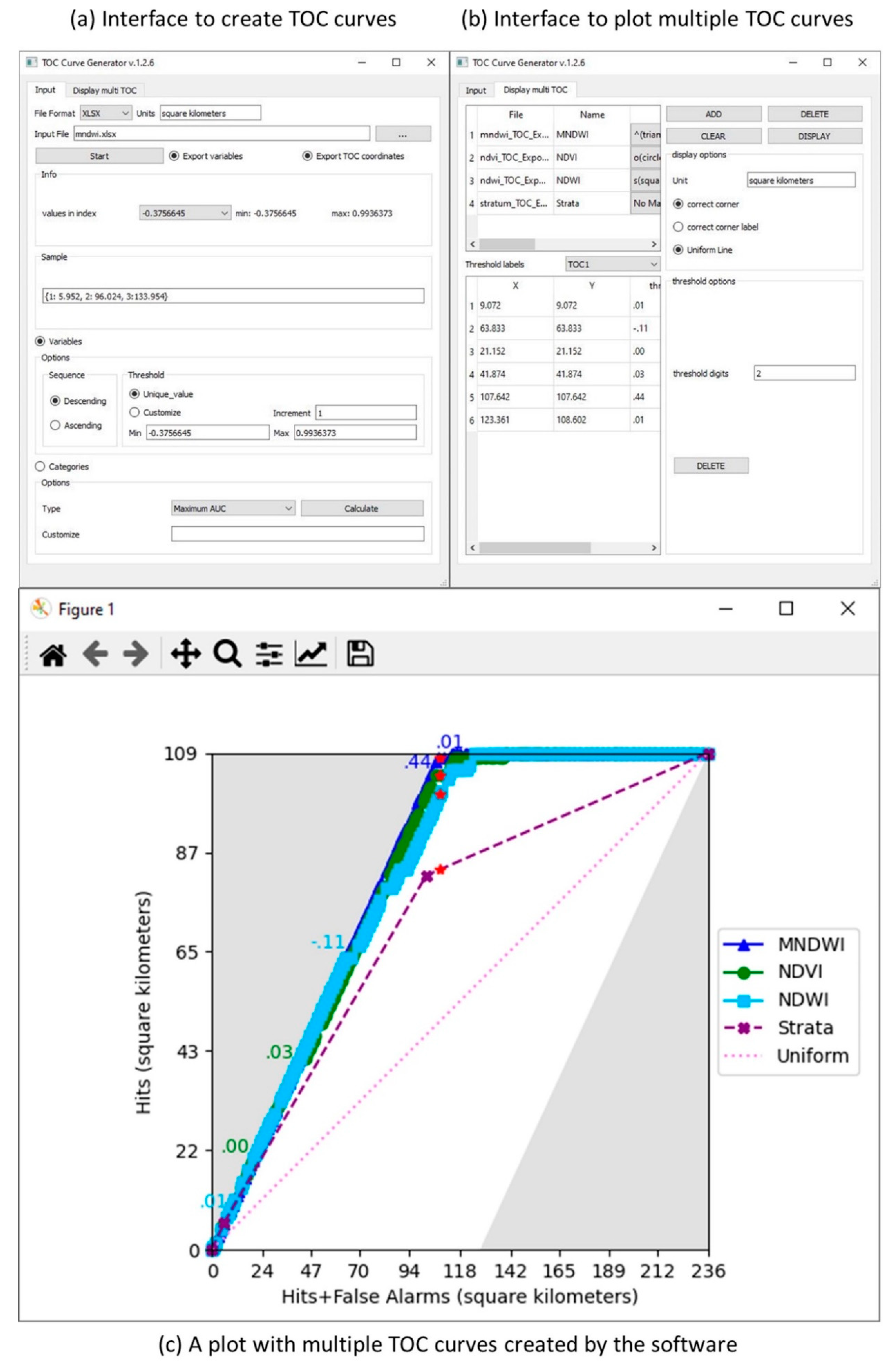
4.4. Software
4.5. Limitations and Next Steps
5. Conclusions
Author Contributions
Funding
Acknowledgments
Conflicts of Interest
References
- Tellman, B.; Sullivan, J.A.; Kuhn, C.; Kettner, A.J.; Doyle, C.S.; Brakenridge, G.R.; Erickson, T.A.; Slayback, D.A. Satellite imaging reveals increased proportion of population exposed to floods. Nature 2021, 596, 80–86. [Google Scholar] [CrossRef]
- Townsend, J.R.G.; Justice, C.O. Analysis of the Dynamics of African Vegetation Using the Normalized Difference Vegetation Index. Int. J. Remote Sens. 1986, 7, 1435–1445. [Google Scholar] [CrossRef]
- McFeeters, S.K. The Use of the Normalized Difference Water Index (NDWI) in the Delineation of Open Water Features. Int. J. Remote Sens. 1996, 17, 1425–1432. [Google Scholar] [CrossRef]
- Xu, H. Modification of Normalised Difference Water Index (NDWI) to Enhance Open Water Features in Remotely Sensed Imagery. Int. J. Remote Sens. 2006, 27, 3025–3033. [Google Scholar] [CrossRef]
- Leiden, J.; Sorn, S.; Hem, S.; Huy, R.; Buchy, P.; Tarantola, A.; Capelle, J. Assessing the performance of remotely-sensed flooding indicators and their potential contribution to early warning for leptospirosis in Cambodia. PLoS ONE 2017, 12, e0181044. [Google Scholar] [CrossRef] [PubMed] [Green Version]
- Sivanpillai, R.; Jacobs, K.M.; Mattilio, C.M.; Piskorski, E.V. Rapid flood inundation mapping by differencing water indices from pre- and post-flood Landsat images. Front. Earth Sci. 2021, 15, e0181044. [Google Scholar] [CrossRef]
- Feyisa, G.L.; Meilby, H.; Fensholt, R.; Proud, S.R. Automated Water Extraction Index: A New Technique for Surface Water Mapping Using Landsat Imagery. Remote Sens. Environ. 2014, 140, 23–35. [Google Scholar] [CrossRef]
- Munasinghe, D.; Cohen, S.; Huang, Y.; Tsang, Y.-P.; Zhang, J.; Fang, Z. Intercomparison of Satellite Remote Sensing-Based Flood Inundation Mapping Techniques. J. Am. Water Resour. Assoc. 2018, 54, 834–846. [Google Scholar] [CrossRef]
- Ji, L.; Zhang, L.; Wylie, B. Analysis of Dynamic Thresholds for the Normalized Difference Water Index. Photogramm. Eng. Remote Sens. 2009, 75, 1307–1317. [Google Scholar] [CrossRef]
- Pontius Jr, R.G.; Si, K. The Total Operating Characteristic to Measure Diagnostic Ability for Multiple Thresholds. Int. J. Geogr. Inf. Sci. 2014, 28, 570–583. [Google Scholar] [CrossRef]
- Cushman, S.A.; Macdonald, E.A.; Landguth, E.L.; Malhi, Y.; Macdonald, D.W. Multiple-Scale Prediction of Forest Loss Risk across Borneo. Landsc. Ecol. 2017, 32, 1581–1598. [Google Scholar] [CrossRef] [Green Version]
- Dustin, D.L.; Jacobson, P.C. Predicting the Extent of Lakeshore Development Using GIS Datasets. Lake Reserv. Manag. 2015, 31, 169–179. [Google Scholar] [CrossRef]
- Harati, S.; Pérez, L.; Molowny-Horas, R.; Pontius Jr, R.G. Validating Models of One-Way Land Change: An Example Case of Forest Insect Disturbance. Landsc. Ecol. 2021, 36, 2919–2935. [Google Scholar] [CrossRef]
- Kamusoko, C.; Gamba, J. Simulating Urban Growth Using a Random Forest-Cellular Automata (RF-CA) Model. IJGI 2015, 4, 447–470. [Google Scholar] [CrossRef]
- Shafizadeh-Moghadam, H.; Minaei, M.; Pontius Jr, R.G.; Asghari, A.; Dadashpoor, H. Integrating a Forward Feature Selection Algorithm, Random Forest, and Cellular Automata to Extrapolate Urban Growth in the Tehran-Karaj Region of Iran. Comput. Environ. Urban Syst. 2021, 87, 101595. [Google Scholar] [CrossRef]
- Swets, J.A. Measuring the Accuracy of Diagnostic Systems. Science 1988, 240, 1285–1293. [Google Scholar] [CrossRef] [PubMed] [Green Version]
- Swets, J.A.; Dawes, R.M.; Monahan, J. Better DECISIONS through SCIENCE. Sci. Am. 2000, 283, 82–87. [Google Scholar] [CrossRef]
- Olofsson, P.; Foody, G.M.; Herold, M.; Stehman, S.V.; Woodcock, C.E.; Wulder, M.A. Good Practices for Estimating Area and Assessing Accuracy of Land Change. Remote Sens. Environ. 2014, 148, 42–57. [Google Scholar] [CrossRef]
- Vox Media. What the Historic Midwest Floods Look Like from Space—And from the Ground. 2019. Available online: https://www.vox.com/energy-and-environment/2019/3/18/18271101/nebraska-flooding-photos (accessed on 24 September 2021).
- Pontius Jr, R.G.; Millones, M. Death to Kappa: Birth of Quantity Disagreement and Allocation Disagreement for Accuracy Assessment. Int. J. Remote Sens. 2011, 32, 4407–4429. [Google Scholar] [CrossRef]
- Foody, G.M. Explaining the Unsuitability of the Kappa Coefficient in the Assessment and Comparison of the Accuracy of Thematic Maps Obtained by Image Classification. Remote Sens. Environ. 2020, 239, 111630. [Google Scholar] [CrossRef]
- Fielding, A.H.; Bell, J.F. A Review of Methods for the Assessment of Prediction Errors in Conservation Presence/Absence Models. Environ. Conserv. 1997, 24, 38–49. [Google Scholar] [CrossRef]
- Liu, Z. TOC Curve Generator. 2020. Available online: https://lazygis.github.io/projects/TOCCurveGenerator (accessed on 24 September 2021).
- Pontius Jr, R.G.; Santacruz, A.; Tayyebi, A.; Parmentier, B. TOC: Total Operating Characteristic Curve and ROC Curve. 2015. Available online: https://cran.r-project.org/web/packages/TOC (accessed on 24 September 2021).
- Pontius Jr, R.G.; Parmentier, B. Recommendations for using the relative operating characteristic (ROC). Landsc. Ecol. 1997, 29, 367–382. [Google Scholar] [CrossRef]


| Observation | Stratum | Size | Weight | Reference | Index | Rank |
|---|---|---|---|---|---|---|
| 1 | 1 | 20 | 10 | 1 | 11 | 1 |
| 2 | 2 | 40 | 5 | 1 | 22 | 2 |
| 3 | 1 | 20 | 10 | 0 | 31 | 3 |
| 4 | 2 | 40 | 5 | 1 | 42 | 4 |
| 5 | 2 | 40 | 5 | 1 | 52 | 5 |
| 6 | 2 | 40 | 5 | 1 | 52 | 5 |
| 7 | 2 | 40 | 5 | 0 | 52 | 5 |
| 8 | 3 | 40 | 10 | 1 | 63 | 6 |
| 9 | 2 | 40 | 5 | 0 | 72 | 7 |
| 10 | 2 | 40 | 5 | 0 | 72 | 7 |
| 11 | 2 | 40 | 5 | 0 | 72 | 7 |
| 12 | 3 | 40 | 10 | 0 | 83 | 8 |
| 13 | 3 | 40 | 10 | 0 | 93 | 9 |
| 14 | 3 | 40 | 10 | 0 | 93 | 9 |
| Symbol | Meaning |
|---|---|
| Dj | Size of Diagnosed Presence at rank j |
| Hj | Size of Hits at rank j |
| j | Rank for a point on the TOC curve where 0 indicates the point at the origin, 1 indicates the first point near the origin, and J indicates the last point at the top right of the TOC |
| J | Number of unique index values among the observations |
| m | Identifier for stratum = 1, 2, …, M |
| M | Number of strata |
| nm | Number of observations in stratum m |
| Number of observations in stratum m diagnosed as a presence at rank j | |
| Number of observations in stratum m diagnosed correctly as a presence at rank j | |
| Sm | Size of stratum m |
| Tj | Threshold value at rank j |
| Wm | Weight as size per observation for observations in stratum m |
| Criterion to Select Threshold | Metric’s Expression |
|---|---|
| Minimum Quantity Difference | |F − M| |
| Minimum Weighted Cost | f F + m M |
| Maximum Correct | H + C |
| Maximum Odds Ratio | |
| Maximum Intersection over Union | |
| Maximum F1 Score | |
| Maximum Kappa | |
| Maximum Phi |
Publisher’s Note: MDPI stays neutral with regard to jurisdictional claims in published maps and institutional affiliations. |
© 2021 by the authors. Licensee MDPI, Basel, Switzerland. This article is an open access article distributed under the terms and conditions of the Creative Commons Attribution (CC BY) license (https://creativecommons.org/licenses/by/4.0/).
Share and Cite
Liu, Z.; Pontius Jr, R.G. The Total Operating Characteristic from Stratified Random Sampling with an Application to Flood Mapping. Remote Sens. 2021, 13, 3922. https://doi.org/10.3390/rs13193922
Liu Z, Pontius Jr RG. The Total Operating Characteristic from Stratified Random Sampling with an Application to Flood Mapping. Remote Sensing. 2021; 13(19):3922. https://doi.org/10.3390/rs13193922
Chicago/Turabian StyleLiu, Zhen, and Robert Gilmore Pontius Jr. 2021. "The Total Operating Characteristic from Stratified Random Sampling with an Application to Flood Mapping" Remote Sensing 13, no. 19: 3922. https://doi.org/10.3390/rs13193922
APA StyleLiu, Z., & Pontius Jr, R. G. (2021). The Total Operating Characteristic from Stratified Random Sampling with an Application to Flood Mapping. Remote Sensing, 13(19), 3922. https://doi.org/10.3390/rs13193922