
LR-TSDet: Towards Tiny Ship Detection in Low-Resolution Remote Sensing Images


Abstract
:
1. Introduction
- An effective detector, LR-TSDet, is proposed to achieve tiny ship detection in low-resolution RSIs; this detector is equipped with a filtered feature aggregation (FFA) module, a hierarchical-atrous spatial pyramid (HASP) module and the IoU-Joint loss.
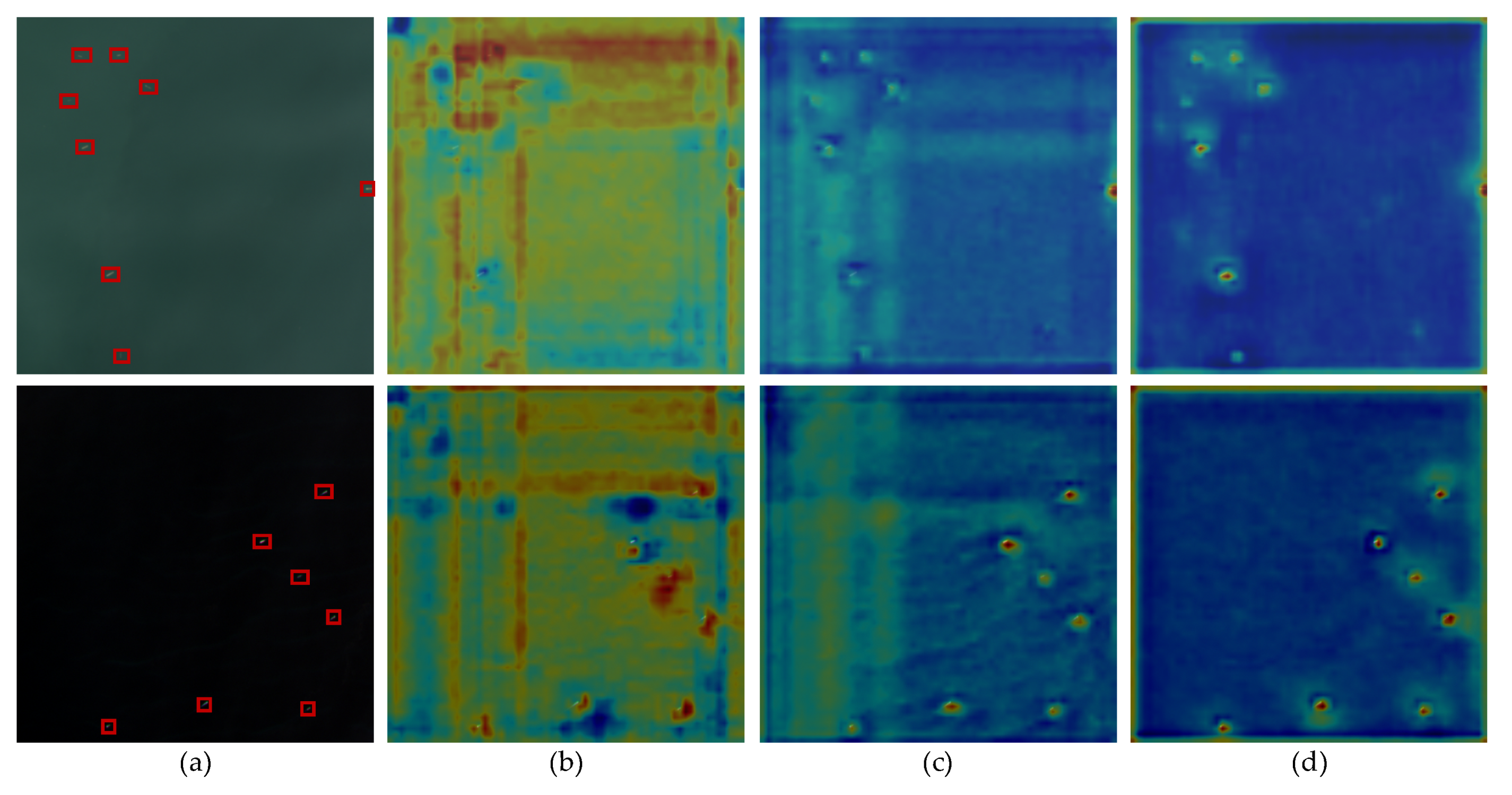
- The FFA module is plugged into the FPN, which aims to suppress the interference of redundant background noise and highlight the response of regions of interest by learning global context information.
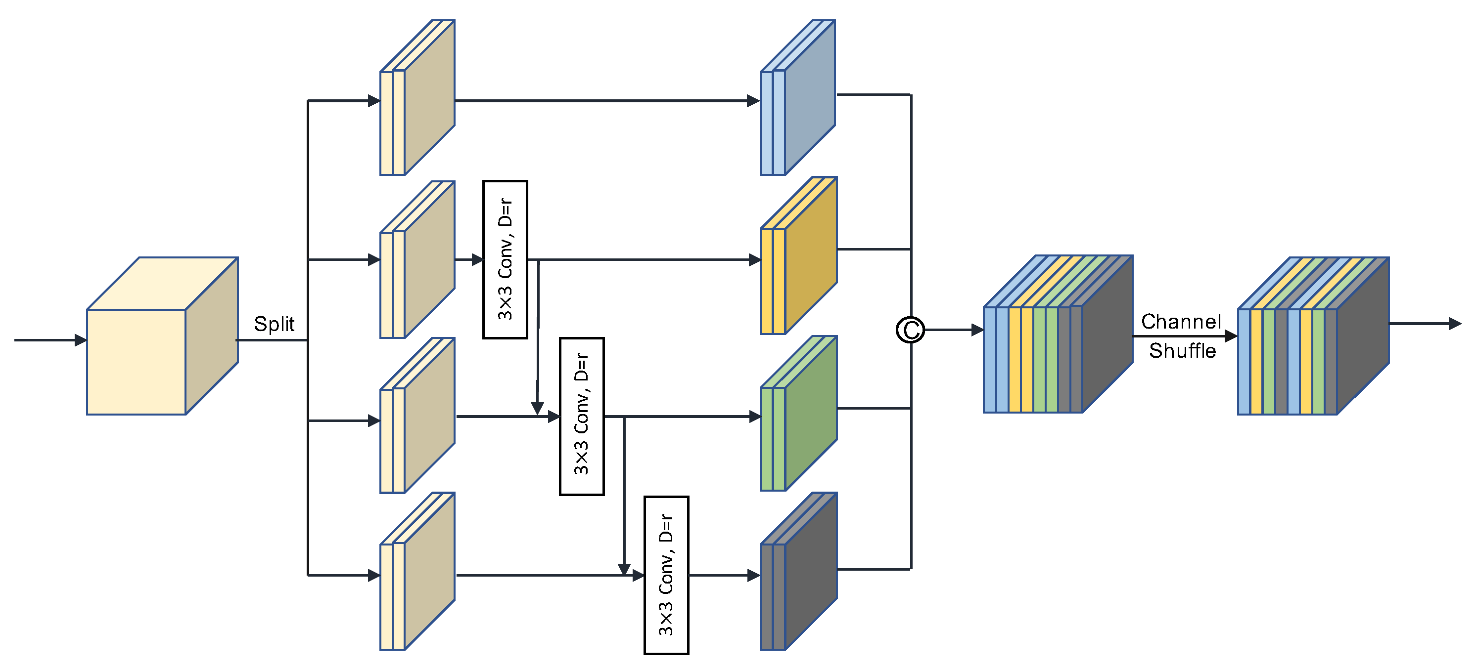
- The HASP module is designed to extract multi-scale local semantic information through aggregating features with different receptive fields.
- The IoU-Joint loss utilizes the IoU score to jointly optimize the classification and regression subnets, further refining the multi-task training process.
- Extensive experiments on our built datasets, GF1-LRSD and DOTA-Ship, validate the performance of our proposed method, which outperforms other comparison methods by a large margin.
2. Related Work
2.1. Object Detection in Remote Sensing Images
2.2. Tiny Object Detection
3. Methods
3.1. Overview
3.2. Filtered Feature Aggregation (FFA) Module
3.3. Hierarchical-Atrous Spatial Pyramid (HASP)
3.4. Loss Function Design
3.4.1. IoU-Joint Classification Loss
3.4.2. Bounding-Box Regression Loss
4. Experiments
4.1. Dataset
4.1.1. GF1-LRSD
Construction Process
- Raw Data Acquisition and PreprocessingGaofen–1 (GF–1) is an optical remote sensing satellite equipped with four 16 m resolution multispectral cameras which can obtain rich remote sensing images. Meanwhile, its complex imaging environment increases the difficulty of detection compared to other data. In order to build a sufficiently effective dataset, we collected a total of 145 wide–field–of–view (WFV) scenes of 1A level with a resolution of 16 m to filter the needed targets. The images with 12,000 × 12,000 pixels are 16-bit and have four bands (the extra is near-infrared), which are difficult to directly apply to the network. Figure 7 shows the detailed data processing flow. We converted the 16-bit data into 8-bit and cropped the large-scale images into a set of slices with the size of . Different from the regular sliding window mechanism, we directly cut the image without overlap for efficiency. As a result, nearly 83,520 sub-images were obtained. To enhance the contrast of images, we used the truncated linear stretch method for quantification, calculated as follows:where and denote the pixel value at in the c-th band of the input and output image, respectively. The is finally limited to 0∼255 to meet the standard format. and are the truncated upper and lower thresholds.
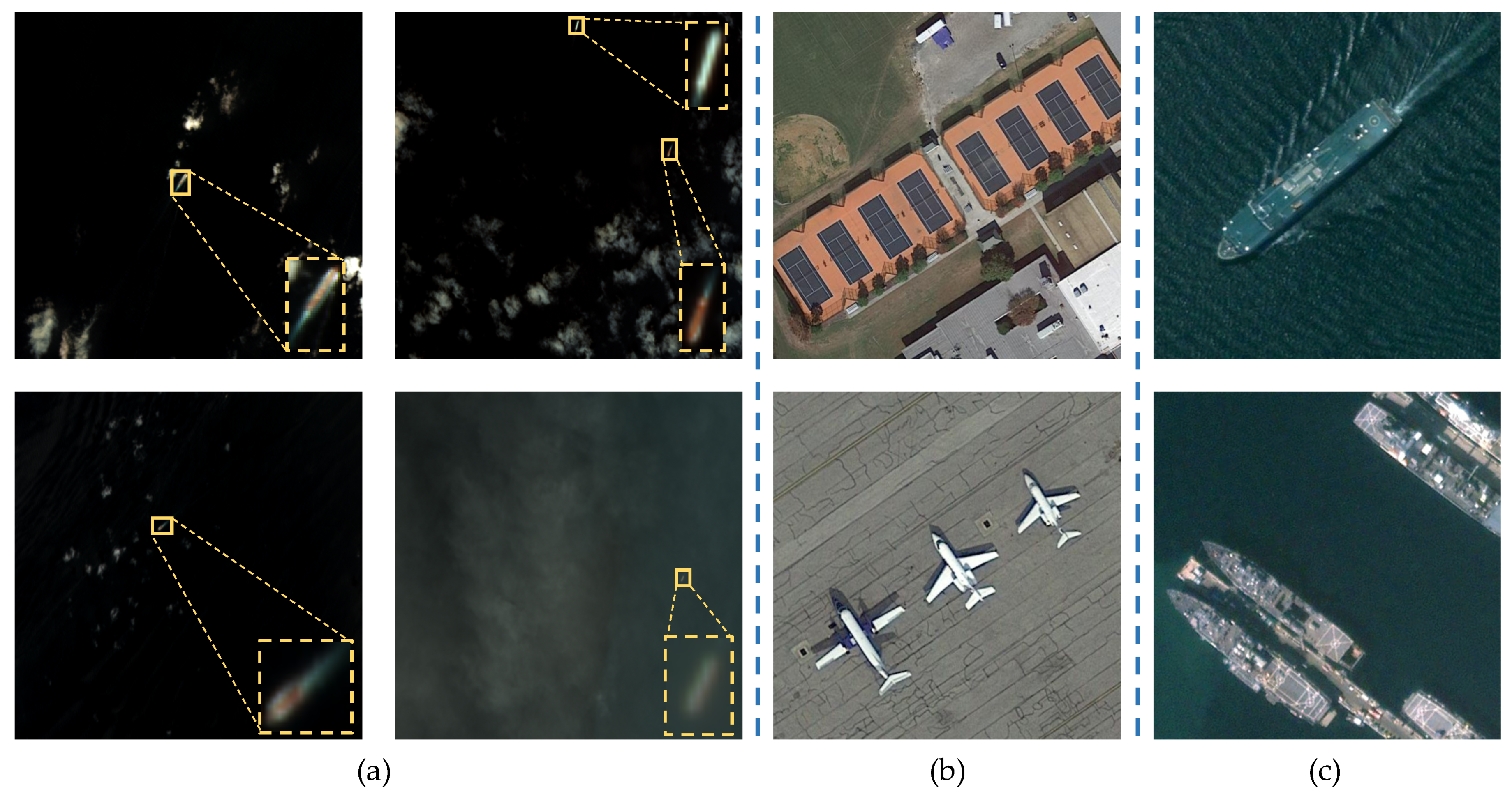
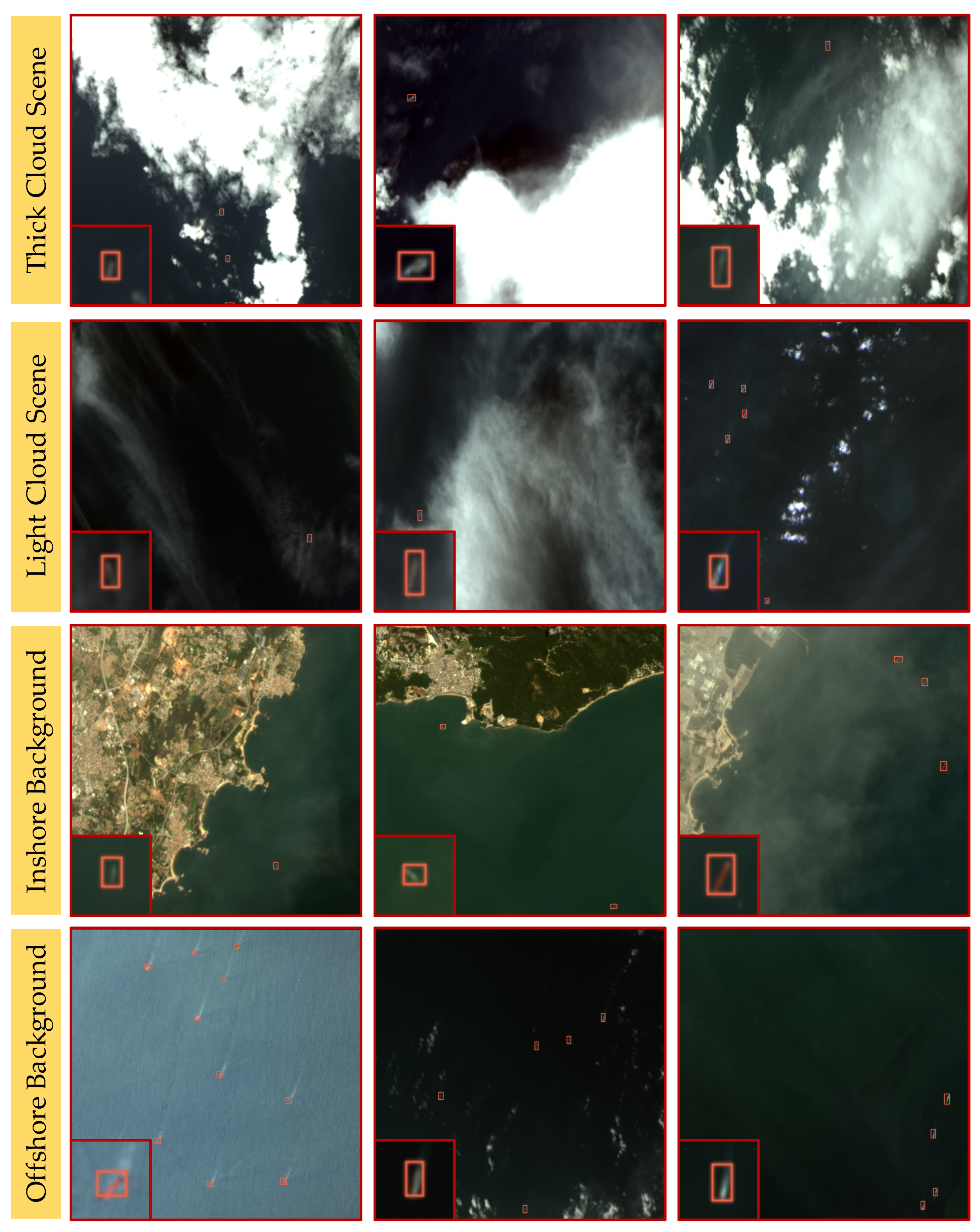
- Image AnnotationWe kept the data organization the same as PASCAL VOC [23] for convenience, wherein is used to describe the labeled bounding box. Let and denote the coordinates of the top-left and bottom-right corners of the bounding box, respectively. The toolbox LabelImg [70] was used to finish the annotation, and we used the horizontal rectangular box to locate the objects. After the identification and correction by experts, we collected, in total, 4406 images and 7172 labeled instances labeled as ship. For dataset splits, 3/5, 1/5, 1/5 of the images were used to form the training set, validation set and test set. Some samples are shown in Figure 1a.
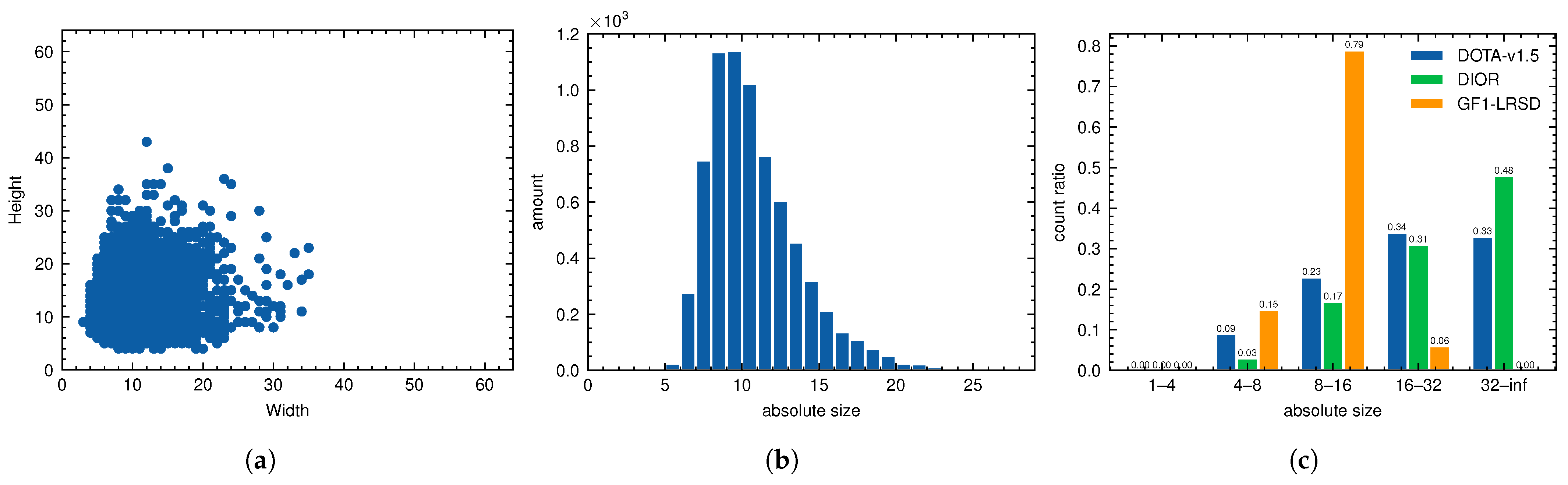
Dataset Statistics
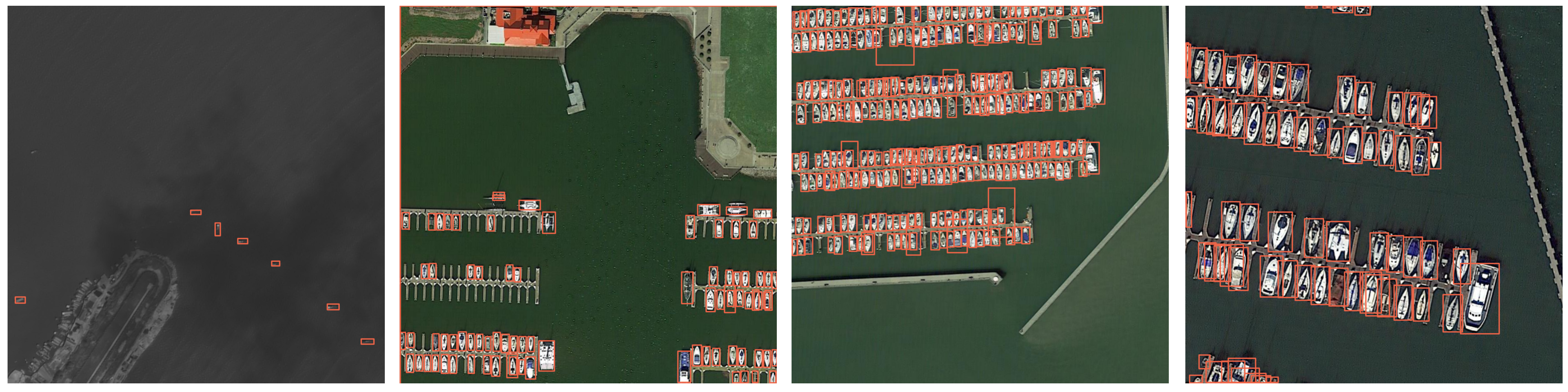
4.1.2. DOTA-Ship
4.2. Implementation Details
4.3. Evaluation Metrics
4.4. Ablation Studies
4.4.1. RetinaNet as Baseline
4.4.2. Individual Contributions of Each Component
- Efficacy of FFA. As discussed in the previous section, FFA processes the feature maps of each residual stage, aiming to suppress the non-object responses. We first applied FFA to the baseline, and it lead to a considerable gain of 1.29 AP, as shown in Experiment #2 in Table 3. FFA utilizes non-local blocks [34] to capture long-range dependencies, which is helpful to obtain global contextual information. Meanwhile, as a kind of attention mechanism, FFA could enhance the feature expression of targets and make it more discriminative.
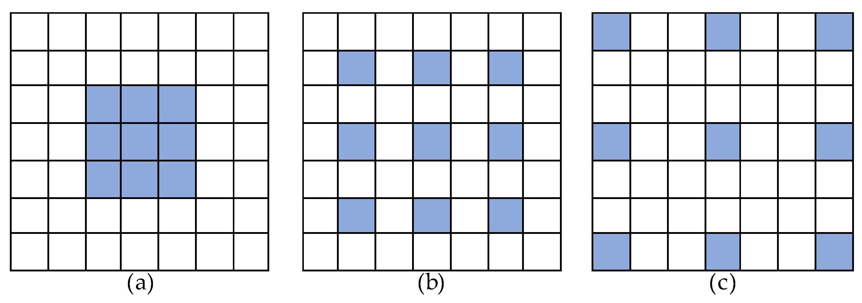
- Influence of HASP. The purpose of designing HASP was to obtain more abundant semantic information while maintaining the resolution of feature maps. To verify its impact, we added HASP on the basis of Experiment #2, and the result is shown in Experiment #3 in Table 3. The detection AP was improved by 0.83 (81.04 → 81.87). HASP aggregates four parallel hierarchical-atrous convolution blocks (HACB) to obtain multi-scale information, where HACB consists of cascaded group dilation convolution. Furthermore, the integration of FFA and HASP further boosted the performance by 2.12, as shown in Experiment {#1, #3} in Table 3.
- Effect of the loss function. As analyzed above, our network is optimized by a multi-task loss, including the classification loss and regression loss. The default setting was focal loss [26] and smooth loss [38] in our experiments. As can be seen in Experiment {#3, #4, #5, #6} in Table 3, both losses contributed to the improvement of the final detection AP. By replacing focal loss with IoU-Joint loss, the network achieved an AP of 82.66, 0.79 higher than the default setting (81.87 vs. 82.66). The reason is that the IoU-Joint loss merges the localization score (i.e., IoU) into the calculation of classification loss, which could strengthen the connection between the two detection branches. Similarly, the performance was improved by 0.75 (81.87 → 82.62) by replacing smooth loss with GIoU loss. The GIoU loss treats the position information as a whole during training, which could result in more accurate training effects. It is worth mentioning that the combination of the two losses brought different degrees of improvement of the detection AP (82.66 → 83.87, 82.62 → 83.87). Finally, the LR-TSDet achieved the best performance of 83.87 AP, which outperformed the baseline by 4.12 AP, demonstrating the effectiveness of the proposed strategies.
4.4.3. Evaluation of HASP
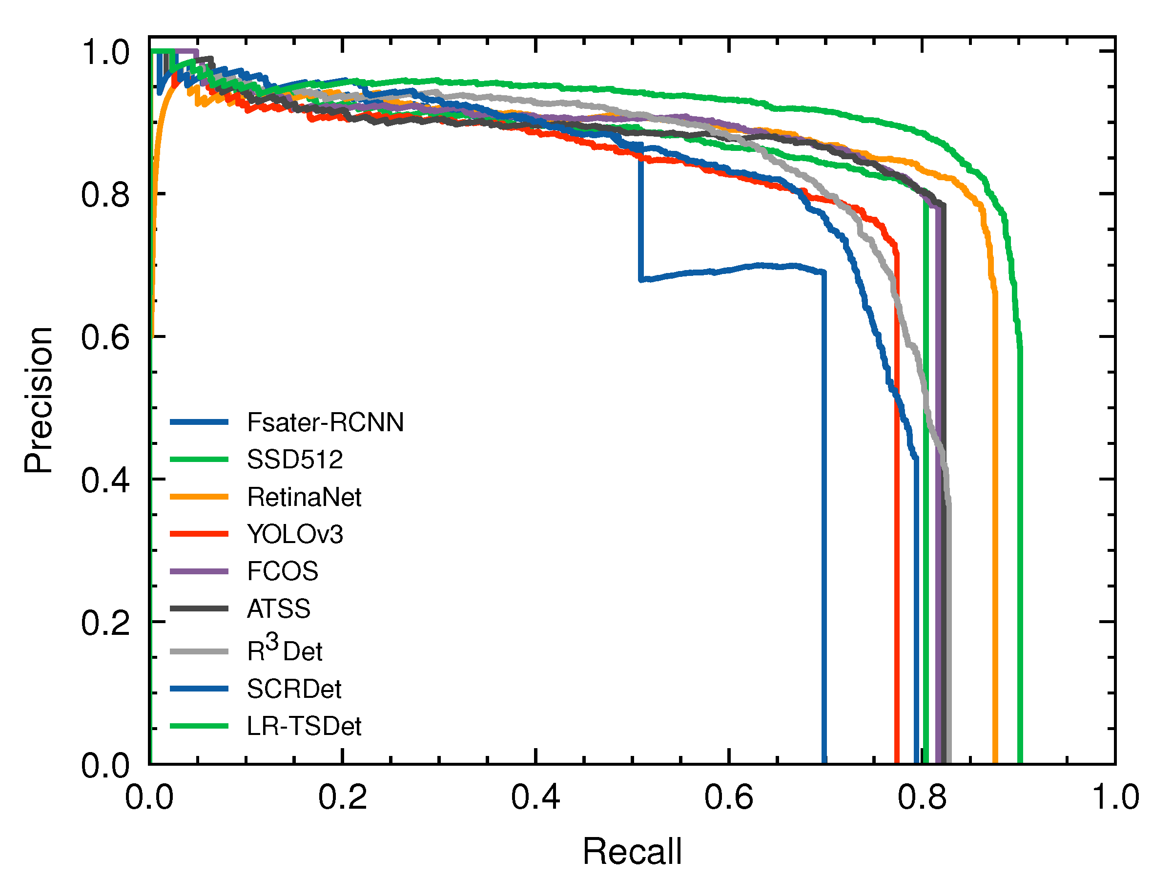
4.5. Comparisons with Other Approaches
4.5.1. Experiments on LR-TSDet
4.5.2. Experiments on DOTA-Ship
5. Conclusions
Author Contributions
Funding
Data Availability Statement
Conflicts of Interest
References
- Cheng, G.; Han, J. A survey on object detection in optical remote sensing images. ISPRS J. Photogramm. Remote Sens. 2016, 117, 11–28. [Google Scholar] [CrossRef] [Green Version]
- Xia, G.S.; Bai, X.; Ding, J.; Zhu, Z.; Belongie, S.; Luo, J.; Datcu, M.; Pelillo, M.; Zhang, L. DOTA: A Large-Scale Dataset for Object Detection in Aerial Images. In Proceedings of the IEEE Conference on Computer Vision and Pattern Recognition (CVPR), Salt Lake City, UT, USA, 18–22 June 2018. [Google Scholar]
- Li, K.; Wan, G.; Cheng, G.; Meng, L.; Han, J. Object detection in optical remote sensing images: A survey and a new benchmark. ISPRS J. Photogramm. Remote Sens. 2020, 159, 296–307. [Google Scholar] [CrossRef]
- Yang, X.; Sun, H.; Fu, K.; Yang, J.; Sun, X.; Yan, M.; Guo, Z. Automatic ship detection in remote sensing images from google earth of complex scenes based on multiscale rotation dense feature pyramid networks. Remote Sens. 2018, 10, 132. [Google Scholar] [CrossRef] [Green Version]
- Zhang, Z.; Guo, W.; Zhu, S.; Yu, W. Toward arbitrary-oriented ship detection with rotated region proposal and discrimination networks. IEEE Geosci. Remote Sens. Lett. 2018, 15, 1745–1749. [Google Scholar] [CrossRef]
- Liu, L.; Shi, Z. Airplane detection based on rotation invariant and sparse coding in remote sensing images. Optik 2014, 125, 5327–5333. [Google Scholar] [CrossRef]
- Li, Y.; Fu, K.; Sun, H.; Sun, X. An aircraft detection framework based on reinforcement learning and convolutional neural networks in remote sensing images. Remote Sens. 2018, 10, 243. [Google Scholar] [CrossRef] [Green Version]
- Zhang, L.; Shi, Z.; Wu, J. A hierarchical oil tank detector with deep surrounding features for high-resolution optical satellite imagery. IEEE J. Sel. Top. Appl. Earth Obs. Remote Sens. 2015, 8, 4895–4909. [Google Scholar] [CrossRef]
- Ok, A.O.; Başeski, E. Circular oil tank detection from panchromatic satellite images: A new automated approach. IEEE Geosci. Remote Sens. Lett. 2015, 12, 1347–1351. [Google Scholar] [CrossRef]
- Xia, G.S.; Hu, J.; Hu, F.; Shi, B.; Bai, X.; Zhong, Y.; Zhang, L.; Lu, X. AID: A benchmark data set for performance evaluation of aerial scene classification. IEEE Trans. Geosci. Remote Sens. 2017, 55, 3965–3981. [Google Scholar] [CrossRef] [Green Version]
- Diakogiannis, F.I.; Waldner, F.; Caccetta, P.; Wu, C. ResUNet-a: A deep learning framework for semantic segmentation of remotely sensed data. ISPRS J. Photogramm. Remote Sens. 2020, 162, 94–114. [Google Scholar] [CrossRef] [Green Version]
- Van Etten, A. You only look twice: Rapid multi-scale object detection in satellite imagery. arXiv 2018, arXiv:1805.09512. [Google Scholar]
- Pang, J.; Li, C.; Shi, J.; Xu, Z.; Feng, H. R2-CNN: Fast Tiny Object Detection in Large-Scale Remote Sensing Images. IEEE Trans. Geosci. Remote Sens. 2019, 57, 5512–5524. [Google Scholar] [CrossRef] [Green Version]
- Shao, J.; Du, B.; Wu, C.; Zhang, L. Tracking objects from satellite videos: A velocity feature based correlation filter. IEEE Trans. Geosci. Remote Sens. 2019, 57, 7860–7871. [Google Scholar] [CrossRef]
- Long, G.; Chen, X.Q. A method for automatic detection of ships in harbor area in high-resolution remote sensing image. Comput. Simul. 2007, 24, 198–201. [Google Scholar]
- Xu, J.; Sun, X.; Zhang, D.; Fu, K. Automatic detection of inshore ships in high-resolution remote sensing images using robust invariant generalized Hough transform. IEEE Geosci. Remote Sens. Lett. 2014, 11, 2070–2074. [Google Scholar]
- Dalal, N.; Triggs, B. Histograms of oriented gradients for human detection. In Proceedings of the 2005 IEEE Computer Society Conference on Computer Vision and Pattern Recognition (CVPR’05), San Diego, CA, USA, 20–26 June 2005; Volume 1, pp. 886–893. [Google Scholar]
- Liao, S.; Zhu, X.; Lei, Z.; Zhang, L.; Li, S.Z. Learning multi-scale block local binary patterns for face recognition. In Proceedings of the International Conference on Biometrics, Seoul, Korea, 27–29 August 2007; pp. 828–837. [Google Scholar]
- Lowe, D. Object recognition from local scale-invariant features. In Proceedings of the Seventh IEEE International Conference on Computer Vision, Kerkyra, Greece, 20–27 September 1999; Volume 2, pp. 1150–1157. [Google Scholar] [CrossRef]
- Yang, F.; Xu, Q.; Li, B. Ship detection from optical satellite images based on saliency segmentation and structure-LBP feature. IEEE Geosci. Remote Sens. Lett. 2017, 14, 602–606. [Google Scholar] [CrossRef]
- Freund, Y.; Schapire, R.E. A decision-theoretic generalization of on-line learning and an application to boosting. J. Comput. Syst. Sci. 1997, 55, 119–139. [Google Scholar] [CrossRef] [Green Version]
- Deng, J.; Dong, W.; Socher, R.; Li, L.J.; Li, K.; Fei-Fei, L. ImageNet: A large-scale hierarchical image database. In Proceedings of the 2009 IEEE Conference on Computer Vision and Pattern Recognition, Miami, FL, USA, 20–25 June 2009; pp. 248–255. [Google Scholar] [CrossRef] [Green Version]
- Everingham, M.; Van Gool, L.; Williams, C.K.; Winn, J.; Zisserman, A. The pascal visual object classes (VOC) challenge. Int. J. Comput. Vis. 2010, 88, 303–338. [Google Scholar] [CrossRef] [Green Version]
- Lin, T.Y.; Maire, M.; Belongie, S.; Hays, J.; Perona, P.; Ramanan, D.; Dollár, P.; Zitnick, C.L. Microsoft coco: Common objects in context. In Proceedings of the European Conference on Computer Vision, Zurich, Switzerland, 6–12 September 2014; pp. 740–755. [Google Scholar]
- Ren, S.; He, K.; Girshick, R.; Sun, J. Faster R-CNN: Towards Real-Time Object Detection with Region Proposal Networks. IEEE Trans. Pattern Anal. Mach. Intell. 2017, 39, 1137–1149. [Google Scholar] [CrossRef] [Green Version]
- Lin, T.Y.; Goyal, P.; Girshick, R.; He, K.; Dollár, P. Focal Loss for Dense Object Detection. In Proceedings of the 2017 IEEE International Conference on Computer Vision (ICCV), Venice, Italy, 22–29 October 2017; pp. 2999–3007. [Google Scholar] [CrossRef] [Green Version]
- Lam, D.; Kuzma, R.; McGee, K.; Dooley, S.; Laielli, M.; Klaric, M.; Bulatov, Y.; McCord, B. xview: Objects in context in overhead imagery. arXiv 2018, arXiv:1802.07856. [Google Scholar]
- Liu, Z.; Yuan, L.; Weng, L.; Yang, Y. A High Resolution Optical Satellite Image Dataset for Ship Recognition and Some New Baselines. In Proceedings of the 6th International Conference on Pattern Recognition Applications and Methods—ICPRAM, Porto, Portugal, 24–26 February 2017; pp. 324–331. [Google Scholar] [CrossRef]
- Ding, J.; Xue, N.; Long, Y.; Xia, G.S.; Lu, Q. Learning roi transformer for oriented object detection in aerial images. In Proceedings of the IEEE/CVF Conference on Computer Vision and Pattern Recognition, Long Beach, CA, USA, 16–20 June 2019; pp. 2849–2858. [Google Scholar]
- Yang, X.; Yan, J.; Feng, Z.; He, T. R3Det: Refined Single-Stage Detector with Feature Refinement for Rotating Object. In Proceedings of the AAAI Conference on Artificial Intelligence, Palo Alto, CA, USA, 2–9 February 2021; Volume 35, pp. 3163–3171. [Google Scholar]
- Wang, J.; Yang, W.; Guo, H.; Zhang, R.; Xia, G.S. Tiny Object Detection in Aerial Images. In Proceedings of the 2020 25th International Conference on Pattern Recognition (ICPR), Milan, Italy, 10–15 January 2021; pp. 3791–3798. [Google Scholar]
- Yang, X.; Hou, L.; Zhou, Y.; Wang, W.; Yan, J. Dense Label Encoding for Boundary Discontinuity Free Rotation Detection. In Proceedings of the IEEE Computer Vision and Pattern Recognition (CVPR), Online, 19–25 June 2021; pp. 15819–15829. [Google Scholar]
- Lin, T.Y.; Dollár, P.; Girshick, R.; He, K.; Hariharan, B.; Belongie, S. Feature Pyramid Networks for Object Detection. In Proceedings of the 2017 IEEE Conference on Computer Vision and Pattern Recognition (CVPR), Honolulu, HI, USA, 21–26 July 2017; pp. 936–944. [Google Scholar] [CrossRef] [Green Version]
- Wang, X.; Girshick, R.; Gupta, A.; He, K. Non-local Neural Networks. In Proceedings of the 2018 IEEE/CVF Conference on Computer Vision and Pattern Recognition, Salt Lake City, UT, USA, 18–22 June 2018; pp. 7794–7803. [Google Scholar] [CrossRef] [Green Version]
- Yu, F.; Koltun, V. Multi-Scale Context Aggregation by Dilated Convolutions. In Proceedings of the International Conference on Learning Representations (ICLR), San Juan, PR, USA, 2–4 May 2016. [Google Scholar]
- Gao, S.; Cheng, M.M.; Zhao, K.; Zhang, X.Y.; Yang, M.H.; Torr, P.H. Res2net: A new multi-scale backbone architecture. arXiv 2019, arXiv:1904.01169. [Google Scholar] [CrossRef] [PubMed] [Green Version]
- Li, X.; Wang, W.; Wu, L.; Chen, S.; Hu, X.; Li, J.; Tang, J.; Yang, J. Generalized Focal Loss: Learning Qualified and Distributed Bounding Boxes for Dense Object Detection. arXiv 2020, arXiv:2006.04388. [Google Scholar]
- Girshick, R. Fast R-CNN. In Proceedings of the IEEE International Conference on Computer Vision (ICCV), Santiago, Chile, 7–13 December 2015. [Google Scholar]
- Liu, W.; Anguelov, D.; Erhan, D.; Szegedy, C.; Reed, S.; Fu, C.Y.; Berg, A.C. SSD: Single Shot MultiBox Detector; ECCV: Amsterdam, The Netherlands, 8–16 October 2016. [Google Scholar]
- Redmon, J.; Farhadi, A. YOLOv3: An Incremental Improvement. arXiv 2018, arXiv:1804.02767. [Google Scholar]
- Pang, J.; Chen, K.; Shi, J.; Feng, H.; Ouyang, W.; Lin, D. Libra r-cnn: Towards balanced learning for object detection. In Proceedings of the IEEE/CVF Conference on Computer Vision and Pattern Recognition, Long Beach, CA, USA, 16–20 June 2019; pp. 821–830. [Google Scholar]
- Zhang, G.; Lu, S.; Zhang, W. CAD-Net: A context-aware detection network for objects in remote sensing imagery. IEEE Trans. Geosci. Remote Sens. 2019, 57, 10015–10024. [Google Scholar] [CrossRef] [Green Version]
- An, Q.; Pan, Z.; Liu, L.; You, H. DRBox-v2: An improved detector with rotatable boxes for target detection in SAR images. IEEE Trans. Geosci. Remote Sens. 2019, 57, 8333–8349. [Google Scholar] [CrossRef]
- Yang, X.; Yan, J.; Qi, M.; Wang, W.; Xiaopeng, Z.; Qi, T. Rethinking Rotated Object Detection with Gaussian Wasserstein Distance Loss. In Proceedings of the International Conference on Machine Learning (ICML), Online, 18–24 July 2021. [Google Scholar]
- Xu, Y.; Fu, M.; Wang, Q.; Wang, Y.; Chen, K.; Xia, G.S.; Bai, X. Gliding vertex on the horizontal bounding box for multi-oriented object detection. arXiv 2020, arXiv:1911.09358. [Google Scholar] [CrossRef] [Green Version]
- Han, J.; Ding, J.; Li, J.; Xia, G.S. Align deep features for oriented object detection. arXiv 2021, arXiv:2008.09397. [Google Scholar]
- Tian, Z.; Shen, C.; Chen, H.; He, T. FCOS: Fully Convolutional One-Stage Object Detection. In Proceedings of the IEEE/CVF International Conference on Computer Vision (ICCV), Seoul, Korea, 27 October–2 November 2019. [Google Scholar]
- Zhou, X.; Wang, D.; Krähenbühl, P. Objects as points. arXiv 2019, arXiv:1904.07850. [Google Scholar]
- Law, H.; Deng, J. Cornernet: Detecting objects as paired keypoints. In Proceedings of the European Conference on Computer Vision (ECCV), Munich, Germany, 8–14 September 2018; pp. 734–750. [Google Scholar]
- Qiu, H.; Ma, Y.; Li, Z.; Liu, S.; Sun, J. Borderdet: Border feature for dense object detection. In Proceedings of the European Conference on Computer Vision, Glasgow, UK, 23–28 August 2020; pp. 549–564. [Google Scholar]
- Wei, H.; Zhang, Y.; Chang, Z.; Li, H.; Wang, H.; Sun, X. Oriented objects as pairs of middle lines. ISPRS J. Photogramm. Remote Sens. 2020, 169, 268–279. [Google Scholar] [CrossRef]
- Lin, Y.; Feng, P.; Guan, J.; Wang, W.; Chambers, J. IENet: Interacting embranchment one stage anchor free detector for orientation aerial object detection. arXiv 2019, arXiv:1912.00969. [Google Scholar]
- Xiao, Z.; Qian, L.; Shao, W.; Tan, X.; Wang, K. Axis Learning for Orientated Objects Detection in Aerial Images. Remote Sens. 2020, 12, 908. [Google Scholar] [CrossRef] [Green Version]
- Yang, Y.; Pan, Z.; Hu, Y.; Ding, C. CPS-Det: An Anchor-Free Based Rotation Detector for Ship Detection. Remote Sens. 2021, 13, 2208. [Google Scholar] [CrossRef]
- Kisantal, M.; Wojna, Z.; Murawski, J.; Naruniec, J.; Cho, K. Augmentation for small object detection. arXiv 2019, arXiv:1902.07296. [Google Scholar]
- Singh, B.; Davis, L.S. An analysis of scale invariance in object detection snip. In Proceedings of the IEEE Conference on Computer Vision and Pattern Recognition, Salt Lake City, UT, USA, 18–22 June 2018; pp. 3578–3587. [Google Scholar]
- Noh, J.; Bae, W.; Lee, W.; Seo, J.; Kim, G. Better to follow, follow to be better: Towards precise supervision of feature super-resolution for small object detection. In Proceedings of the IEEE/CVF International Conference on Computer Vision, Seoul, Korea, 27 October–2 November 2019; pp. 9725–9734. [Google Scholar]
- Yu, X.; Gong, Y.; Jiang, N.; Ye, Q.; Han, Z. Scale match for tiny person detection. In Proceedings of the IEEE/CVF Winter Conference on Applications of Computer Vision, The Westin Snowmass Resort, Snowmass Village, CO, USA, 1–5 March 2020; pp. 1257–1265. [Google Scholar]
- Yang, X.; Yang, J.; Yan, J.; Zhang, Y.; Zhang, T.; Guo, Z.; Sun, X.; Fu, K. Scrdet: Towards more robust detection for small, cluttered and rotated objects. In Proceedings of the IEEE/CVF International Conference on Computer Vision, Seoul, Korea, 27–28 October 2019; pp. 8232–8241. [Google Scholar]
- Hu, P.; Ramanan, D. Finding Tiny Faces. In Proceedings of the IEEE Conference on Computer Vision and Pattern Recognition (CVPR), Honolulu, HI, USA, 21–26 July 2017. [Google Scholar]
- He, K.; Zhang, X.; Ren, S.; Sun, J. Deep Residual Learning for Image Recognition. In Proceedings of the 2016 IEEE Conference on Computer Vision and Pattern Recognition (CVPR), Las Vegas, NV, USA, 27–30 June 2016; pp. 770–778. [Google Scholar] [CrossRef] [Green Version]
- Tan, M.; Le, Q. Efficientnet: Rethinking model scaling for convolutional neural networks. In Proceedings of the International Conference on Machine Learning, Long Beach, CA, USA, 9–15 June 2019; PMLR, 2019; pp. 6105–6114. [Google Scholar]
- Liu, Z.; Lin, Y.; Cao, Y.; Hu, H.; Wei, Y.; Zhang, Z.; Lin, S.; Guo, B. Swin Transformer: Hierarchical Vision Transformer using Shifted Windows. arXiv 2021, arXiv:2103.14030. [Google Scholar]
- Long, J.; Shelhamer, E.; Darrell, T. Fully convolutional networks for semantic segmentation. In Proceedings of the IEEE Conference on Computer Vision and Pattern Recognition, Boston, MA, USA, 7–12 June 2015; pp. 3431–3440. [Google Scholar]
- Vaswani, A.; Shazeer, N.; Parmar, N.; Uszkoreit, J.; Jones, L.; Gomez, A.N.; Kaiser, L.u.; Polosukhin, I. Attention is All you Need. In Advances in Neural Information Processing Systems; Guyon, I., Luxburg, U.V., Bengio, S., Wallach, H., Fergus, R., Vishwanathan, S., Garnett, R., Eds.; Curran Associates, Inc.: Long Beach, CA, USA, 2017; Volume 30. [Google Scholar]
- Wu, Y.; He, K. Group normalization. In Proceedings of the European Conference on Computer Vision (ECCV), Munich, Germany, 8–14 September 2018; pp. 3–19. [Google Scholar]
- Nair, V.; Hinton, G.E. Rectified Linear Units Improve Restricted Boltzmann Machines; Icml: Haifa, Israel, 21–24 June 2010. [Google Scholar]
- Ma, N.; Zhang, X.; Zheng, H.T.; Sun, J. Shufflenet v2: Practical guidelines for efficient cnn architecture design. In Proceedings of the European Conference on Computer Vision (ECCV), Munich, Germany, 8–14 September 2018; pp. 116–131. [Google Scholar]
- Rezatofighi, H.; Tsoi, N.; Gwak, J.; Sadeghian, A.; Reid, I.; Savarese, S. Generalized Intersection Over Union: A Metric and a Loss for Bounding Box Regression. In Proceedings of the IEEE/CVF Conference on Computer Vision and Pattern Recognition (CVPR), Long Beach, CA, USA, 16–20 June 2019. [Google Scholar]
- Tzutalin, D. LabelImg. GitHub Repository. 2015, Volume 6. Available online: https://github.com/tzutalin/labelImg (accessed on 5 October 2015).
- Chen, K.; Wang, J.; Pang, J.; Cao, Y.; Xiong, Y.; Li, X.; Sun, S.; Feng, W.; Liu, Z.; Xu, J.; et al. MMDetection: Open MMLab Detection Toolbox and Benchmark. arXiv 2019, arXiv:1906.07155. [Google Scholar]
- Wang, P.; Chen, P.; Yuan, Y.; Liu, D.; Huang, Z.; Hou, X.; Cottrell, G. Understanding convolution for semantic segmentation. In Proceedings of the 2018 IEEE winter conference on applications of computer vision (WACV), Lake Tahoe, NV, USA, 12–15 March 2018; pp. 1451–1460. [Google Scholar]
- Zhang, S.; Chi, C.; Yao, Y.; Lei, Z.; Li, S.Z. Bridging the Gap Between Anchor-based and Anchor-free Detection via Adaptive Training Sample Selection. arXiv 2020, arXiv:1912.02424. [Google Scholar]


| Dataset | Absolute Size | Relative Size |
|---|---|---|
| DOTA-v1.0 trainval | 55.3 ± 63.1 | 0.028 ± 0.034 |
| DOTA-v1.5 trainval | 34.0 ± 47.8 | 0.016 ± 0.026 |
| DIOR | 65.7 ± 91.8 | 0.082 ± 0.115 |
| HRSC2016 | 140.6 ± 67.9 | 0.149 ± 0.072 |
| GF1-LRSD | 10.9 ± 3.0 | 0.021 ± 0.006 |
| Model | FPN | Head | AP (%) | FLOPs (G) | #Params (M) |
|---|---|---|---|---|---|
| RetinaNet-D | {P3, P4, P5, P6, P7} | - | 79.00 | 52.28 | 36.1 |
| RetinaNet-B | {P3, P4, P5} | + GN | 79.75 | 51.57 | 30.8 |
| ID | FFA | HASP | IoU-Joint Loss | GIoU Loss | AP (%) |
|---|---|---|---|---|---|
| #1 | - | - | - | - | 79.75 |
| #2 | ✓ | - | - | - | 81.04 |
| #3 | ✓ | ✓ | - | - | 81.87 |
| #4 | ✓ | ✓ | ✓ | - | 82.66 |
| #5 | ✓ | ✓ | - | ✓ | 82.62 |
| #6 | ✓ | ✓ | ✓ | ✓ | 83.87 |
| ID | Dilations | HACB | AP (%) |
|---|---|---|---|
| #1 | {1, 1, 1, 1} | ✓ | 82.98 |
| #2 #3 | {1, 2, 3, 4} | - ✓ | 82.84 83.44 |
| #4 #5 | {2, 4, 6, 8} | - ✓ | 83.31 83.87 |
| #6 | {6, 6, 6, 6} | ✓ | 83.15 |
| Method | Backbone | AP (%) | FLOPs (G) | #Params (M) |
|---|---|---|---|---|
| Faster-RCNN [25] | ResNet50 | 60.49 | 63.25 | 41.12 |
| RetinaNet [26] | ResNet50 | 79.00 | 52.28 | 36.10 |
| SSD512 [39] | VGG16 | 72.28 | 87.72 | 24.39 |
| YOLOv3 [40] | DarkNet53 | 67.82 | 49.62 | 61.52 |
| FCOS [47] | ResNet50 | 74.16 | 50.30 | 31.84 |
| ATSS [73] | ResNet50 | 73.84 | 51.52 | 31.89 |
| SCRDet [59] | ResNet50 | 69.29 | - | - |
| R3Det [30] | ResNet50 | 73.04 | - | - |
| LR-TSDet (ours) | ResNet50 | 83.87 | 54.67 | 32.53 |
| Scene | Method | Recall (%) | Precision (%) | AP (%) |
|---|---|---|---|---|
| Offshore | RetinaNet LR-TSDet | 89.64 91.65 | 65.96 66.11 | 81.62 86.43 |
| Inshore | RetinaNet LR-TSDet | 78.46 82.69 | 41.63 42.74 | 65.35 71.30 |
| Method | Backbone | AP (%) |
|---|---|---|
| Faster-RCNN [25] | ResNet50 | 79.49 |
| RetinaNet [26] | ResNet50 | 75.58 |
| SSD512 [39] | VGG16 | 76.92 |
| YOLOv3 [40] | DarkNet53 | 66.17 |
| FCOS [47] | ResNet50 | 77.08 |
| ATSS [73] | ResNet50 | 78.17 |
| SCRDet [59] | ResNet50 | 79.57 |
| R3Det [30] | ResNet50 | 75.15 |
| LR-TSDet (ours) | ResNet50 | 83.62 |
Publisher’s Note: MDPI stays neutral with regard to jurisdictional claims in published maps and institutional affiliations. |
© 2021 by the authors. Licensee MDPI, Basel, Switzerland. This article is an open access article distributed under the terms and conditions of the Creative Commons Attribution (CC BY) license (https://creativecommons.org/licenses/by/4.0/).
Share and Cite
Wu, J.; Pan, Z.; Lei, B.; Hu, Y. LR-TSDet: Towards Tiny Ship Detection in Low-Resolution Remote Sensing Images. Remote Sens. 2021, 13, 3890. https://doi.org/10.3390/rs13193890
Wu J, Pan Z, Lei B, Hu Y. LR-TSDet: Towards Tiny Ship Detection in Low-Resolution Remote Sensing Images. Remote Sensing. 2021; 13(19):3890. https://doi.org/10.3390/rs13193890
Chicago/Turabian StyleWu, Jixiang, Zongxu Pan, Bin Lei, and Yuxin Hu. 2021. "LR-TSDet: Towards Tiny Ship Detection in Low-Resolution Remote Sensing Images" Remote Sensing 13, no. 19: 3890. https://doi.org/10.3390/rs13193890
APA StyleWu, J., Pan, Z., Lei, B., & Hu, Y. (2021). LR-TSDet: Towards Tiny Ship Detection in Low-Resolution Remote Sensing Images. Remote Sensing, 13(19), 3890. https://doi.org/10.3390/rs13193890