
Branch-Pipe: Improving Graph Skeletonization around Branch Points in 3D Point Clouds


Abstract
:1. Introduction
Related Work
2. Methods
2.1. Overview
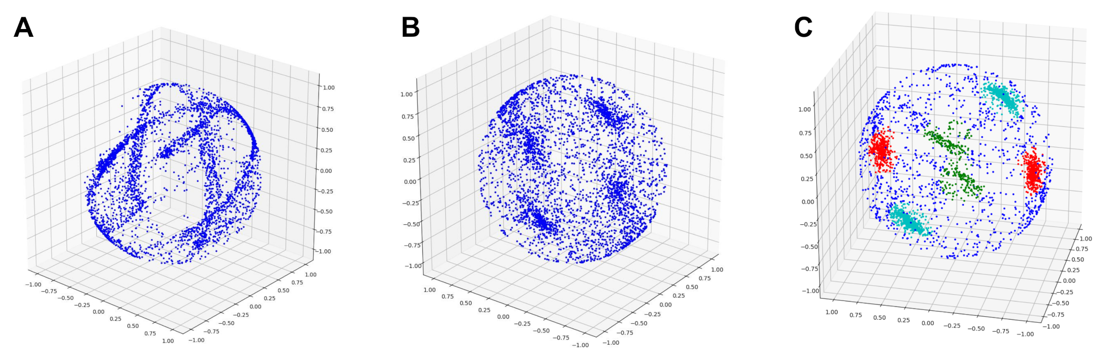
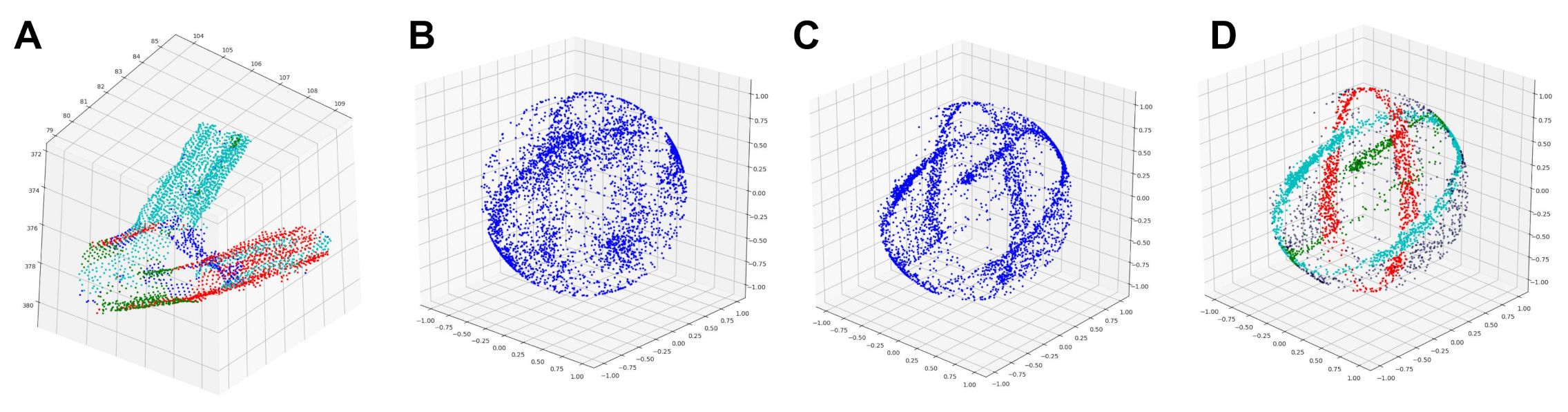
2.2. Gaussian Sphere Mapping
2.3. Sampling of Cylinder Axes
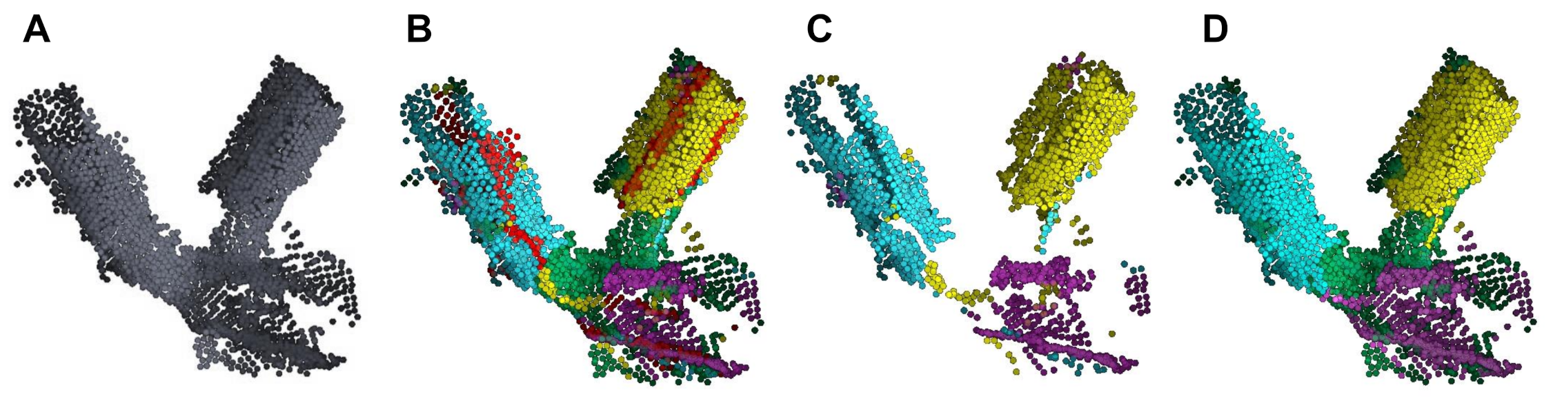
2.4. Clustering Cylinder Axes
2.4.1. A Modified Clustering Algorithm
2.4.2. Dealing with Ambiguous Points
2.5. Final Skeleton Graph
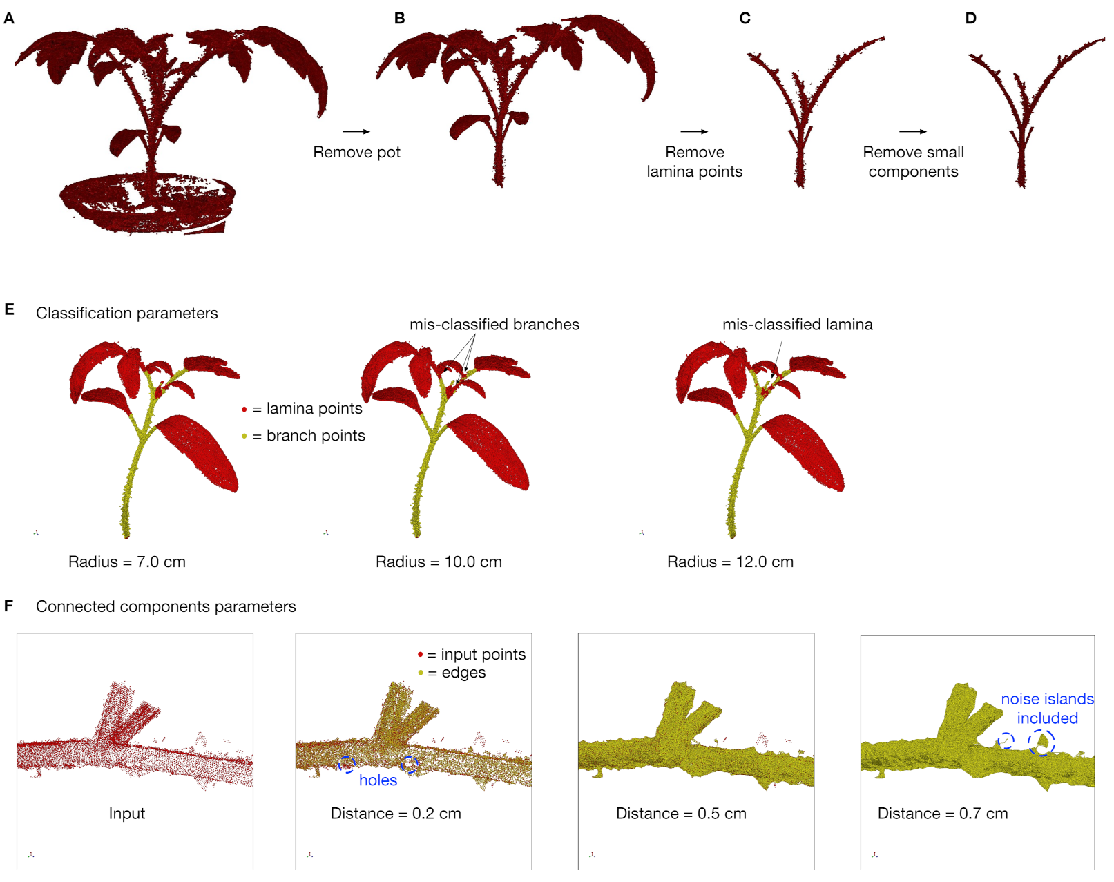
2.6. Plant Data
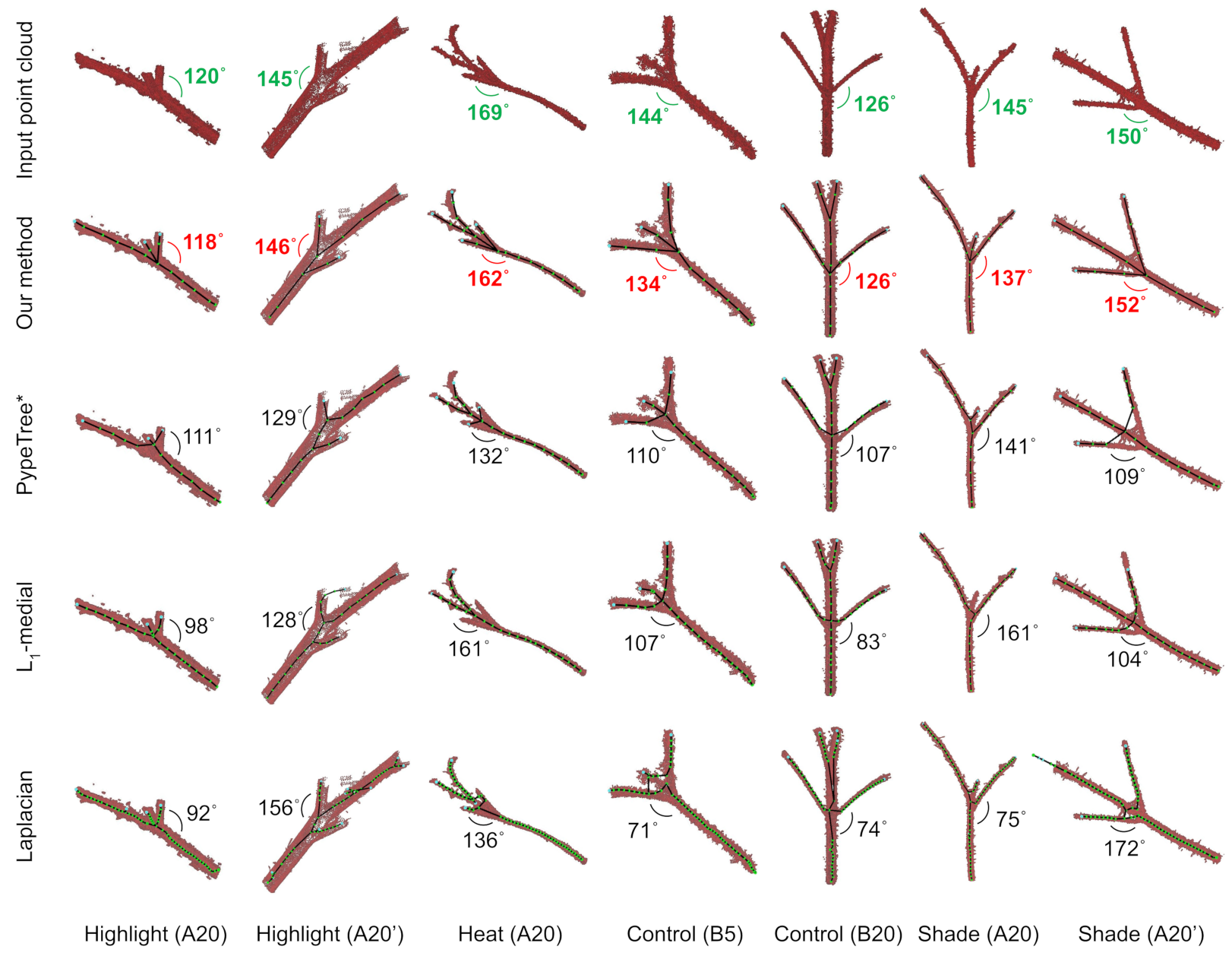
3. Results
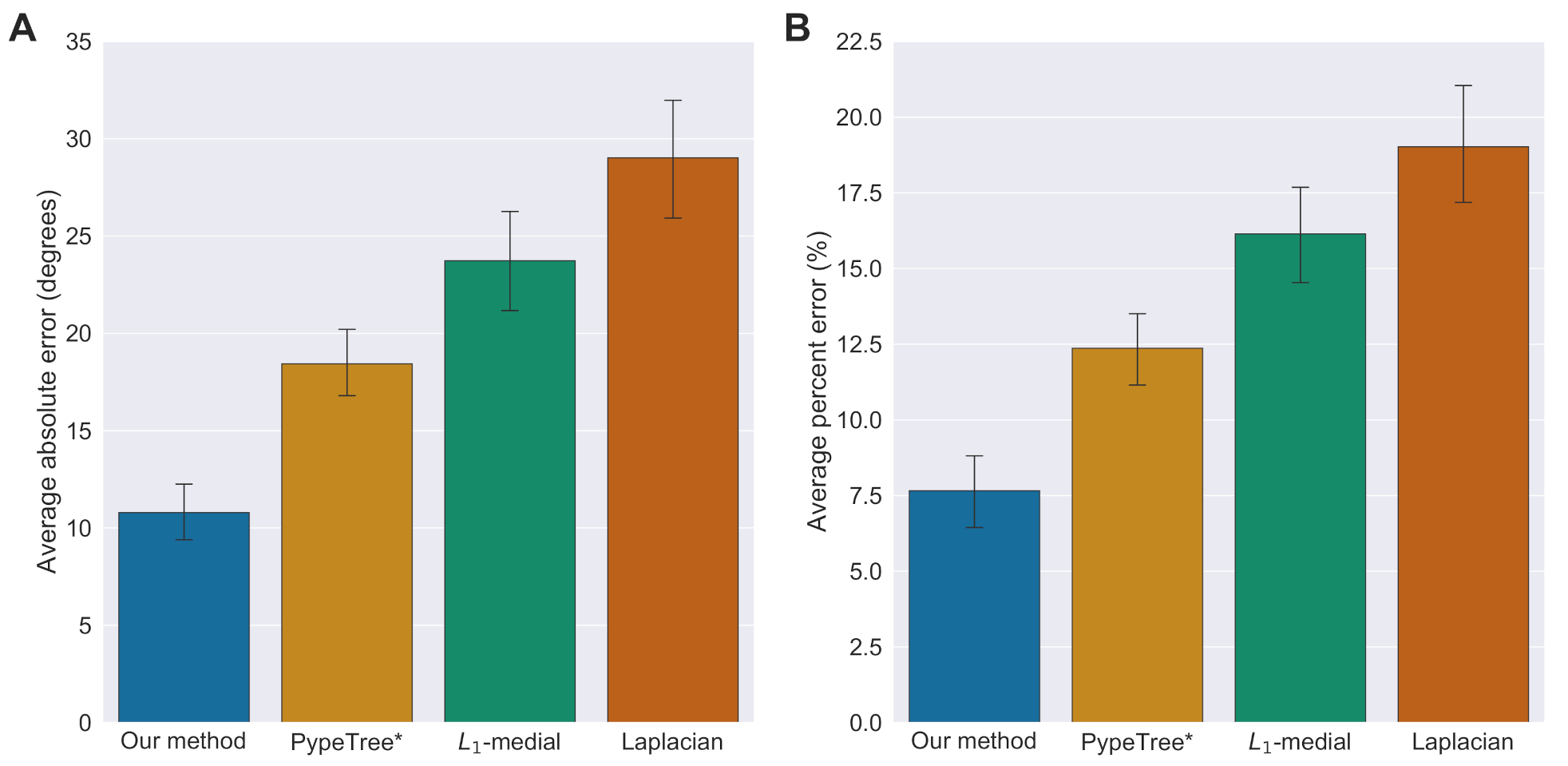
3.1. Accuracy of Branch Angles
3.2. Run-Time Performance
4. Conclusions
Author Contributions
Funding
Institutional Review Board Statement
Informed Consent Statement
Data Availability Statement
Conflicts of Interest
References
- Cornea, N.D.; Silver, D.; Min, P. Curve-Skeleton Properties, Applications, and Algorithms. IEEE Trans. Vis. Comput. Graph. 2007, 13, 530–548. [Google Scholar] [CrossRef] [PubMed] [Green Version]
- Tagliasacchi, A.; Zhang, H.; Cohen-Or, D. Curve Skeleton Extraction from Incomplete Point Cloud. In ACM SIGGRAPH 2009 Papers; Association for Computing Machinery: New York, NY, USA, 2009; pp. 1–9. [Google Scholar]
- Cao, J.; Tagliasacchi, A.; Olson, M.; Zhang, H.; Su, Z. Point Cloud Skeletons via Laplacian Based Contraction. In Proceedings of the 2010 Shape Modeling International Conference, Aix-en-Provence, France, 21–23 June 2010; pp. 187–197. [Google Scholar] [CrossRef] [Green Version]
- Au, O.K.C.; Tai, C.L.; Chu, H.K.; Cohen-Or, D.; Lee, T.Y. Skeleton Extraction by Mesh Contraction. ACM Trans. Graph. 2008, 27, 1–10. [Google Scholar] [CrossRef]
- Delagrange, S.; Jauvin, C.; Rochon, P. PypeTree: A Tool for Reconstructing Tree Perennial Tissues from Point Clouds. Sensors 2014, 14, 4271–4289. [Google Scholar] [CrossRef] [PubMed] [Green Version]
- Verroust, A.; Lazarus, F. Extracting Skeletal Curves from 3D Scattered Data. Vis. Comput. 2000, 16, 15–25. [Google Scholar] [CrossRef]
- Huang, H.; Wu, S.; Cohen-Or, D.; Gong, M.; Zhang, H.; Li, G.; Chen, B. L1-Medial Skeleton of Point Cloud. ACM Trans. Graph. 2013, 32, 1–8. [Google Scholar] [CrossRef] [Green Version]
- Sharf, A.; Lewiner, T.; Shamir, A.; Kobbelt, L. On-the-fly Curve-skeleton Computation for 3D Shapes. In Computer Graphics Forum; Blackwell Publishing Ltd.: Oxford, UK, 2007; Volume 26, pp. 323–328. [Google Scholar]
- Ai, M.; Yao, Y.; Hu, Q.; Wang, Y.; Wang, W. An Automatic Tree Skeleton Extraction Approach Based on Multi-View Slicing Using Terrestrial LiDAR Scans Data. Remote Sens. 2020, 12, 3824. [Google Scholar] [CrossRef]
- Conn, A.; Pedmale, U.V.; Chory, J.; Navlakha, S. High-Resolution Laser Scanning Reveals Plant Architectures That Reflect Universal Network Design Principles. Cell Syst. 2017, 5, 53–62. [Google Scholar] [CrossRef] [PubMed] [Green Version]
- Bucksch, A.; Atta-Boateng, A.; Azihou, A.F.; Battogtokh, D.; Baumgartner, A.; Binder, B.M.; Braybrook, S.A.; Chang, C.; Coneva, V.; DeWitt, T.J.; et al. Morphological plant modeling: Unleashing geometric and topological potential within the plant sciences. Front. Plant Sci. 2017, 8, 900. [Google Scholar] [CrossRef] [PubMed]
- Prusinkiewicz, P.; Lindenmayer, A. The Algorithmic Beauty of Plants; Springer Science & Business Media: Berlin/Heidelberg, Germany, 2012. [Google Scholar]
- Perez-Sanz, F.; Navarro, P.J.; Egea-Cortines, M. Plant Phenomics: An Overview of Image Acquisition Technologies and Image Data Analysis Algorithms. GigaScience 2017, 6, gix092. [Google Scholar] [CrossRef] [Green Version]
- Pieruschka, R.; Schurr, U. Plant phenotyping: Past, present, and future. Plant Phenomics 2019, 2019, 7507131. [Google Scholar] [CrossRef]
- Li, M.; Frank, M.H.; Coneva, V.; Mio, W.; Chitwood, D.H.; Topp, C.N. The Persistent Homology Mathematical Framework Provides Enhanced Genotype-to-Phenotype Associations for Plant Morphology. Plant Physiol. 2018, 177, 1382–1395. [Google Scholar] [CrossRef] [Green Version]
- Gaetan, L.; Serge, C.; Annie, E.; Didier, C.; Frederic, B. Characterization of Whole Plant Leaf Area Properties Using Laser Scanner Point Clouds. In Proceedings of the 2012 IEEE 4th International Symposium on Plant Growth Modeling, Simulation, Visualization and Applications, Shanghai, China, 31 October–3 November 2012; pp. 250–253. [Google Scholar] [CrossRef] [Green Version]
- Xu, H.; Bassel, G.W. Linking Genes to Shape in Plants Using Morphometrics. Annu. Rev. Genet. 2020, 54, 417–437. [Google Scholar] [CrossRef]
- Sun, S.; Li, C.; Paterson, A.H.; Jiang, Y.; Xu, R.; Robertson, J.S.; Snider, J.L.; Chee, P.W. In-Field High Throughput Phenotyping and Cotton Plant Growth Analysis Using LiDAR. Front. Plant Sci. 2018, 9, 16. [Google Scholar] [CrossRef] [Green Version]
- Andújar, D.; Rueda-Ayala, V.; Moreno, H.; Rosell-Polo, J.; Escolá, A.; Valero, C.; Gerhards, R.; Fernández-Quintanilla, C.; Dorado, J.; Griepentrog, H.W. Discriminating Crop, Weeds and Soil Surface with a Terrestrial LIDAR Sensor. Sensors 2013, 13, 14662–14675. [Google Scholar] [CrossRef] [Green Version]
- Mathan, J.; Bhattacharya, J.; Ranjan, A. Enhancing Crop Yield by Optimizing Plant Developmental Features. Development 2016, 143, 3283–3294. [Google Scholar] [CrossRef] [Green Version]
- Giovannetti, M.; Małolepszy, A.; Göschl, C.; Busch, W. Large-Scale Phenotyping of Root Traits in the Model Legume Lotus Japonicus. In Plant Genomics; Springer: New York, NY, USA, 2017; Volume 1610, pp. 155–167. [Google Scholar] [CrossRef]
- Yang, W.; Duan, L.; Chen, G.; Xiong, L.; Liu, Q. Plant phenomics and high-throughput phenotyping: Accelerating rice functional genomics using multidisciplinary technologies. Curr. Opin. Plant Biol. 2013, 16, 180–187. [Google Scholar] [CrossRef]
- Hackenberg, J.; Spiecker, H.; Calders, K.; Disney, M.; Raumonen, P. SimpleTree—An efficient open source tool to build tree models from TLS clouds. Forests 2015, 6, 4245–4294. [Google Scholar] [CrossRef]
- Morsdorf, F.; Meier, E.; Kötz, B.; Itten, K.I.; Dobbertin, M.; Allgöwer, B. LIDAR-based geometric reconstruction of boreal type forest stands at single tree level for forest and wildland fire management. Remote Sens. Environ. 2004, 92, 353–362. [Google Scholar] [CrossRef]
- Zhang, X.; Li, H.; Dai, M.; Ma, W.; Quan, L. Data-driven synthetic modeling of trees. IEEE Trans. Vis. Comput. Graph. 2014, 20, 1214–1226. [Google Scholar] [CrossRef]
- Qiu, R.; Zhou, Q.Y.; Neumann, U. Pipe-Run Extraction and Reconstruction from Point Clouds. In Computer Vision–ECCV 2014; Fleet, D., Pajdla, T., Schiele, B., Tuytelaars, T., Eds.; Springer International Publishing: Cham, Switzerland, 2014; Volume 8691, pp. 17–30. [Google Scholar] [CrossRef] [Green Version]
- Han, X.F.; Jin, J.S.; Wang, M.J.; Jiang, W.; Gao, L.; Xiao, L. A review of algorithms for filtering the 3D point cloud. Signal Process. Image Commun. 2017, 57, 103–112. [Google Scholar] [CrossRef]
- Pauly, M.; Mitra, N.J.; Guibas, L.J. Uncertainty and Variability in Point Cloud Surface Data. In Proceedings of the Eurographics Symposium on Point-Based Graphics, SPBG’04. Zurich, Switzerland, 2–4 June 2004; Eurographics Association: Goslar, Germany, 2004; pp. 77–84. [Google Scholar]
- Xia, S.; Chen, D.; Wang, R.; Li, J.; Zhang, X. Geometric primitives in LiDAR point clouds: A review. IEEE J. Sel. Top. Appl. Earth Obs. Remote Sens. 2020, 13, 685–707. [Google Scholar] [CrossRef]
- Ziamtsov, I.; Navlakha, S. Machine Learning Approaches to Improve Three Basic Plant Phenotyping Tasks Using Three-Dimensional Point Clouds. Plant Physiol. 2019, 181, 1425–1440. [Google Scholar] [CrossRef] [Green Version]
- Hassouna, M.S.; Farag, A.A. Robust centerline extraction framework using level sets. In Proceedings of the 2005 IEEE Computer Society Conference on Computer Vision and Pattern Recognition (CVPR’05), San Diego, CA, USA, 20–25 June 2005; Volume 1, pp. 458–465. [Google Scholar]
- Mei, J.; Zhang, L.; Wu, S.; Wang, Z.; Zhang, L. 3D tree modeling from incomplete point clouds via optimization and L 1-MST. Int. J. Geogr. Inf. Sci. 2017, 31, 999–1021. [Google Scholar] [CrossRef]
- Wang, Z.; Zhang, L.; Fang, T.; Mathiopoulos, P.T.; Qu, H.; Chen, D.; Wang, Y. A structure-aware global optimization method for reconstructing 3-D tree models from terrestrial laser scanning data. IEEE Trans. Geosci. Remote Sens. 2014, 52, 5653–5669. [Google Scholar] [CrossRef]
- Ogniewicz, R.; Ilg, M. Voronoi Skeletons: Theory and Applications. In Proceedings of the 1992 IEEE Computer Society Conference on Computer Vision and Pattern Recognition, Champaign, IL, USA, 15–18 June 1992; pp. 63–69. [Google Scholar] [CrossRef]
- Dey, T.K.; Sun, J. Defining and computing curve-skeletons with medial geodesic function. In Proceedings of the Symposium on Geometry Processing, Cagliari, Italy, 26–28 June 2006; Volume 6, pp. 143–152. [Google Scholar]
- Mitra, N.J.; Nguyen, A. Estimating surface normals in noisy point cloud data. In Proceedings of the Nineteenth Annual Symposium on Computational Geometry, San Diego, CA, USA, 8–10 June 2003; pp. 322–328. [Google Scholar]
- Zhang, J.; Cao, J.; Liu, X.; Wang, J.; Liu, J.; Shi, X. Point cloud normal estimation via low-rank subspace clustering. Comput. Graph. 2013, 37, 697–706. [Google Scholar] [CrossRef]
- Fischler, M.A.; Bolles, R.C. Random Sample Consensus: A Paradigm for Model Fitting with Applications to Image Analysis and Automated Cartography. Commun. ACM 1981, 24, 381–395. [Google Scholar] [CrossRef]
- Marton, Z.C.; Pangercic, D.; Blodow, N.; Kleinehellefort, J.; Beetz, M. General 3D modelling of novel objects from a single view. In Proceedings of the 2010 IEEE/RSJ International Conference on Intelligent Robots and Systems, Taipei, Taiwan, 18–22 October 2010; pp. 3700–3705. [Google Scholar] [CrossRef] [Green Version]
- Comaniciu, D.; Meer, P. Mean Shift: A Robust Approach Toward Feature Space Analysis. IEEE Trans. Pattern Anal. Mach. Intell. 2002, 24, 603–619. [Google Scholar] [CrossRef] [Green Version]
- Conn, A.; Pedmale, U.V.; Chory, J.; Stevens, C.F.; Navlakha, S. A Statistical Description of Plant Shoot Architecture. Curr. Biol. 2017, 27, 2078–2088.e3. [Google Scholar] [CrossRef] [Green Version]
- Rusu, R.B.; Blodow, N.; Beetz, M. Fast Point Feature Histograms (FPFH) for 3D registration. In Proceedings of the 2009 IEEE International Conference on Robotics and Automation, Kobe, Japan, 12–17 May 2009; pp. 3212–3217. [Google Scholar] [CrossRef]
- Nguyen, T.T.; Slaughter, D.C.; Max, N.; Maloof, J.N.; Sinha, N. Structured light-based 3D reconstruction system for plants. Sensors 2015, 15, 18587–18612. [Google Scholar] [CrossRef] [PubMed] [Green Version]
- Ziamtsov, I.; Navlakha, S. Plant 3D (P3D): A Plant Phenotyping Toolkit for 3D Point Clouds. Bioinformatics 2020, 36, 3949–3950. [Google Scholar] [CrossRef]


| Species | Point Cloud | Our Method | PypeTree* | -Medial | Laplacian |
|---|---|---|---|---|---|
| Tomato | Control (B5) | 1.40 | 1.26 | 3.76 | 41.77 |
| Tomato | Control (B20) | 6.13 | 5.25 | 5.69 | 494.49 |
| Tomato | Heat (A20) | 2.51 | 2.06 | 4.05 | 53.91 |
| Tomato | Highlight (A20) | 1.68 | 1.34 | 3.06 | 47.44 |
| Tomato | Highlight (A20’) | 1.89 | 1.62 | 5.22 | 77.95 |
| Tomato | Shade (A20) | 2.68 | 2.19 | 3.05 | 68.12 |
| Tomato | Shade (A20’) | 2.27 | 2.03 | 2.98 | 91.01 |
| Tomato | Drought (A12) | 1.27 | 1.01 | 4.49 | 73.22 |
| Tomato | Highlight (B4) | 0.75 | 0.67 | 3.64 | 20.56 |
| Tomato | Shade (B20) | 9.73 | 7.98 | 9.99 | 491.51 |
| Tobacco | Control (B6) | 0.27 | 0.23 | 4.34 | 13.77 |
| Tobacco | Control (B12) | 0.82 | 0.64 | 4.20 | 21.66 |
| Tobacco | Heat (B6) | 0.25 | 0.19 | 2.42 | 14.98 |
| Tobacco | Heat (B20) | 7.37 | 5.49 | 5.77 | 360.03 |
Publisher’s Note: MDPI stays neutral with regard to jurisdictional claims in published maps and institutional affiliations. |
© 2021 by the authors. Licensee MDPI, Basel, Switzerland. This article is an open access article distributed under the terms and conditions of the Creative Commons Attribution (CC BY) license (https://creativecommons.org/licenses/by/4.0/).
Share and Cite
Ziamtsov, I.; Faizi, K.; Navlakha, S. Branch-Pipe: Improving Graph Skeletonization around Branch Points in 3D Point Clouds. Remote Sens. 2021, 13, 3802. https://doi.org/10.3390/rs13193802
Ziamtsov I, Faizi K, Navlakha S. Branch-Pipe: Improving Graph Skeletonization around Branch Points in 3D Point Clouds. Remote Sensing. 2021; 13(19):3802. https://doi.org/10.3390/rs13193802
Chicago/Turabian StyleZiamtsov, Illia, Kian Faizi, and Saket Navlakha. 2021. "Branch-Pipe: Improving Graph Skeletonization around Branch Points in 3D Point Clouds" Remote Sensing 13, no. 19: 3802. https://doi.org/10.3390/rs13193802
APA StyleZiamtsov, I., Faizi, K., & Navlakha, S. (2021). Branch-Pipe: Improving Graph Skeletonization around Branch Points in 3D Point Clouds. Remote Sensing, 13(19), 3802. https://doi.org/10.3390/rs13193802