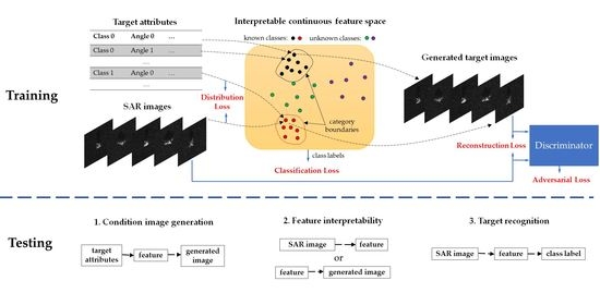
1. Introduction
Automatic target recognition (ATR) is a challenging task for synthetic aperture radar (SAR) [
1,
2]. In general, SAR-ATR may consist of two stages: first extract the representative features of SAR image and then assign the image to a predetermined set of classes using a classifier. The discriminative features are crucial for SAR-ATR and can significantly influence the success of the latter classifier. In the last few decades, lots of feature-extracted technologies have been proposed in SAR-ATR, including but not limited to the principal component analysis (PCA)-based method [
3,
4], the scattering center model (SCM)-based method [
5,
6], sparse representation method [
7,
8], Krawtchouk moments method [
9], and multi-features fusion method [
10]. Different from the traditional technologies which extract the image features manually, the deep learning (DL) technology can automatically extract the image features by combining the feature extractor and the classifier, so the remarkable performance on target recognition can be achieved. Several results on some public data sets for SAR-ATR by using DL (deep learning) have been reported and are far beyond the results by using traditional technologies [
11,
12,
13]. However, there are some obvious limitations on the DL-based SAR-ATR studies at present. On one hand, many of the existing DL models are black boxes that do not explain their predictions in a way that humans can understand, so it is hard to ensure the rationality and reliability of the predictive models. On the other hand, most of the existing SAR target recognition methods suppose that the target classes in the test set have appeared in the training set. However, in a realistic scenario, there probably exist some unknown target classes. The traditional SAR-ATR methods will not work or deteriorate seriously for the unknown classes.
In order to cope with the above challenges, some researches have been done. In [
14,
15], the transfer learning is studied to transfer the knowledge from some SAR data sets with abundant labeled samples to the target task with limited labeled samples. In [
16], the recognition model is firstly trained on the simulated SAR data, and then is transferred to the transferred target task. In [
17,
18], the simulated SAR images are refined to reduce the difference between the simulated image and the real image. Besides the transfer learning methods, the generative networks [
19,
20] are also used to produce the SAR images that are not contained in the training data. All the above studies are helpful to improve the classification results for the case that only few samples of the SAR target classes are available. However, for the target classes with no one sample, the few-shot learning (FSL) methods are valid. To address this issue, several zero-shot learning (ZSL) methods have been studied in SAR-ATR. In [
21,
22], the optical images or the simulated SAR images of the unknown class targets are utilized to provide the aided information for zero-shot target recognition. Without adding extra information, a feature space for SAR-ATR is built based on the known class targets in [
23]. By mapping the SAR images of the unknown class targets into the feature space, the attribute of the target can be explained in some extent. Moreover, the feature space is continuous and is able to generate the target images that are not in the training data, although the generated images are usually obscure. In [
24], a more stable feature space is built which has the better interpretability. The problem in [
23,
24] is the feature space can only explain the unknown class qualitatively, but can’t distinguish the unknown class from the known classes effectively. Open set recognition (OSR) is a similar task as zero-shot recognition. Besides several known classes, OSR takes all the unknown classes as an extra class. In test, it can classify targets of the known classes and reject targets of the unknown classes. Several studies have been done on OSR for SAR targets, such as the support vector machine (SVM)-based methods [
25] and the edge exemplar selection methods [
26,
27]. These methods don’t exploit the strong ability of feature extraction in DL. Recently, a OSR method for SAR-ATR is proposed based on Generative Adversarial Network (GAN) [
28]. A classification branch is added to the discriminator, so the discriminator can provide the target class as well as the score of probability that the target belongs to the known class. However, the recognition accuracy decreases obviously as the number of know classes increases. What is more, the proposed model also lacks transparency and interpretability, like most of existing DL models.
In this paper, we focus on the problem of OSR in SAR-ATR where there is no information about the unknown classes, including the training samples, class number, semantic information, etc. The feature learning method is studied for SAR-ATR, which should classify the known classes, reject the unknown classes and is also explainable in some degree. Inspired by [
23,
24], a feature space which can well represent the attributes of the SAR target and also has the ability of image generation is expected in the paper. Variational Auto-encoder (VAE) [
29,
30] and GAN [
31,
32] are the two most popular deep generative models, which can both generate images by inputting random noise. The noise in VAE is supposed to have some certain distribution and can be seen as the representation of images. VAE is rigorous in theory, but the generated images are often blurry. GAN has no explicit assumption on the noise distribution and can usually produce clear images. However, the input noise in GAN can’t represent the images and the interpretability is not enough. What is more, the traditional VAE and GAN can’t conduct the conditional generation. It is possible to improve the generated image by combining VAE and GAN [
33,
34]. In the paper, a conditional VAE (CVAE) together with GAN (CVAE-GAN) is proposed for feature learning in SAR-ATR. The latent variable space in VAE, where the noise is produced, is selected as the feature space. Both the target representation and classification are conducted in this feature space. The attribute and class label of the target are used as the conditions to control the image generation. An extra discriminator is used to improve the quality of the generated image. Compared with the existing approaches, the proposed CVAE-GAN model can obtain a feature space for SAR-ATR, which has three main advantages.
Condition generation for SAR images. By using the encoder network and the generation network in CVAE-GAN jointly, clear SAR images, which are absent in the training data set, can be generated with the given target class label and target attributes, while the network in [
23] only produces the obscure images. It can be used in data augmentation and benefit for SAR-ATR with limited labeled data.
Feature interpretability in some degree. Different from that of auto-encoder, the latent variable of VAE is continuous in the variable space. Therefore, the latent variable obtained via the encoder network can act as the representation of SAR images and reflects some attributes of the target. The network in [
28] is incapable of the interpretability.
Recognition of unknown classes. Because of the additive angular margin in the feature space, the intra-class distance of the known classes is decreased and the inter-class distance is increased. As a result, it is possible to classify the known classes and recognize the unknown target classes whose features are outside the angular range of the known classes. The networks in [
23,
24] can’t recognize the unknown classes.
The rest of this paper is organized as follows. In
Section 2, the proposed CVAE-GAN is introduced in detail, including the model derivation, loss function and network structure. In
Section 3, experimental results are shown to demonstrate the effectiveness of the proposal. In
Section 4, the results are further discussed compared with the previous studies. The work is concluded in
Section 5.
2. CVAE-GAN for SAR-ATR with Unknown Target Classes
The main objective in this paper is to find an explicable feature space, in which the attributes of the SAR images can be well represented and the unknown classes can be distinguished. The generative model is a good choice to achieve the interpretability. We select VAE as the generative model, because it not only has the generation ability, but also can obtain the feature representation of images. Considering only random images can be generated in the original VAE, in this section, we will firstly derive a conditional VAE model by embedding the target attributes. And then integrate the classification loss and GAN loss into the CVAE model and achieve the CVAE-GAN model. The resultant model encourages the abilities of conditional image generation, feature interpretability and target classification simultaneously. A deep network will be built based on the proposed model in the last.
2.1. CVAE-GAN Model
We expect to generate the corresponding target SAR image with a given class label and some attribute parameters such as the observation angle, resolution, frequency and polarization mode. Let
denote the target image, the class label and the related attribute parameters, respectively. The generation model can be realized by maximizing the conditional log-likelihood function
where
are the prior distribution and posterior distribution of
. According to the idea of VAE, an auxiliary latent variable
is added to represent
. Let
be the posterior distribution of
, and
can be expressed as
where
refers to the (Kullback–Leibler, KL)-divergence between the distributions
and
. Because of the non-negativity of KL-divergence, we can get the variational lower bound of
which is written as
Therefore, the maximization of
can be converted to maximize its variational lower bound, which is further derived as
Consider the latent variable
can be generated with
by
, so the term
in (4) is simplified as
. That means the latent variable
contains the information of target class label and target attribute, so it can be used to generate the corresponding target image. As a result, the generation problem in (1) can be re-expressed as
In Equation (5), the expectation sign is omitted for simplicity. The first term in Equation (5) aims to minimize the difference between the distribution and . As a result, the latent variable produced from will have the information of . This makes it possible for conditional image generation and the latter target classification compared with the original VAE. The purpose of the second term in Equation (5) is to maximize the probability of generating the image from the corresponding which is produced by . The two losses above are called as the distribution loss and the reconstruction loss, respectively, in the following.
Since the latent variable
contains the target class information, it can be used as the recognition feature for target classification. Therefore, a classification loss
is added in Equation (5) and the problem is further expressed as
Considering the generated images via VAE are often blurry, GAN is combined with CVAE in this paper to improve the image quality. Let
be an extra discriminator, and then the problem of the generation model is expressed as
The adversarial loss for the discriminator is expressed as
Equations (7) and (8) are the final objective functions for the CVAE-GAN model, which will be solved alternately in training.
2.2. Realization of Loss Functions
The concrete form of the loss function in Equation (7) is derived in the following.
2.2.1. Distribution Loss
We suppose
and
in the first term of Equation (7) have the normal distribution
and
, respectively. The mean value
and standard deviation
are the functions of
, while
are the functions of
. Different from the standard normal distribution used for all samples in the original VAE, the distributions for different samples can be various based on the target attributes. Therefore, it is possible to distinguish the samples with different target attributes in the feature space. Mark
as
, respectively, for simply, and the distribution loss in (7) can be expressed as
If both
and
are alterable, the possible results of
and
may be both close to 0 in order to maximize
. In this case, the randomness which is expected in VAE will have disappeared. To avoid this problem, we fix
and let
in this paper. And then (9) is revised as
As the latent variable is multidimensional, the final loss is the sum of in all the dimensions.
2.2.2. Reconstruction Loss
Suppose
in the second loss of Equation (7) has the normal distribution
, where
is a function of
and
is a constant. Thus, the reconstruction loss is expressed as
It can be seen from Equation (11) that, the maximization of is equal to the minimization of .
2.2.3. Classification Loss
The cross-entropy loss (CEL) is the commonly used classification loss. For the
th target sample and the corresponding feature
, whose class label is
, the CEL (maximization) is expressed as
where
is the number of the known target classes,
is the score that
belongs to the
th class,
are the weight and bias in the classifier corresponding to the
th class. However, just as stated in the introduction, there may exist some unknown classes in practice and the traditional CEL can’t distinguish them from the known classes. In order to recognize the unknown classes, an idea is to incorporate the margin in the softmax loss functions, which can push the classification boundary closer to the weight vectors and add the inter-class separability. It is a popular line of research for face recognition in recent years [
35,
36,
37,
38,
39,
40]. In this paper, we apply the ArcFace [
40] to add the angular margin for the known classes in the feature space. Let
and
,
is a predetermined constant. And then the classification loss is expressed as
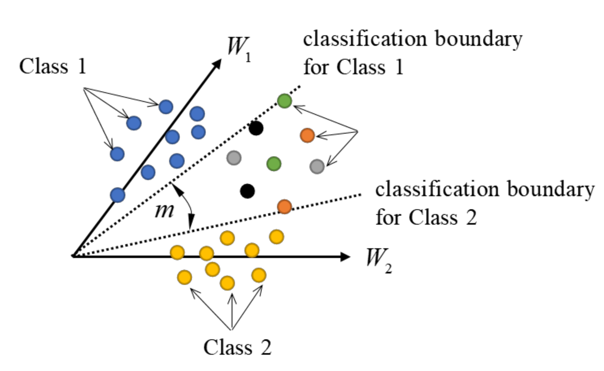
where
,
,
and
are the angles between
and
,
, respectively,
is the additive angular margin. In Equation (13), the different classes can be separated in angle. For the simplest binary classification, the classification boundaries for Class 1 and Class 2 are
and
, respectively. The schematic diagram is shown in
Figure 1. For
, the two classification boundaries coincide with each other and the unknown classes can’t be identified, while
the two classification boundaries are separated and the unknown classes are possible to be distinguished from the known.
The fourth term in Equation (7) is realized by using the traditional GAN loss and more details can be found in [
31].
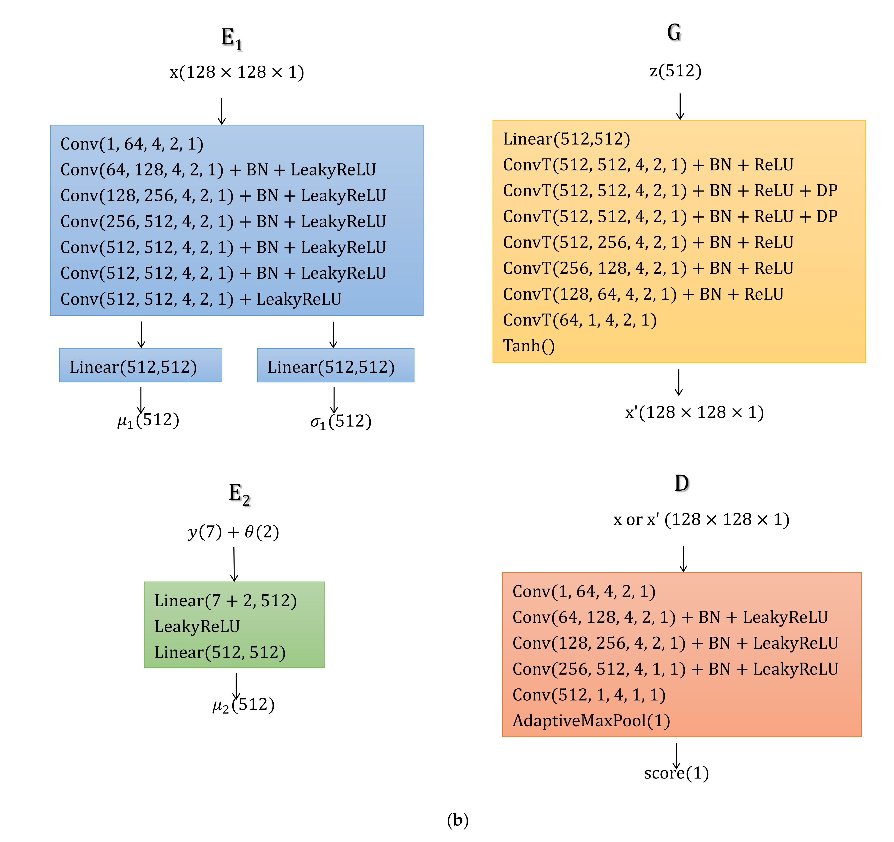
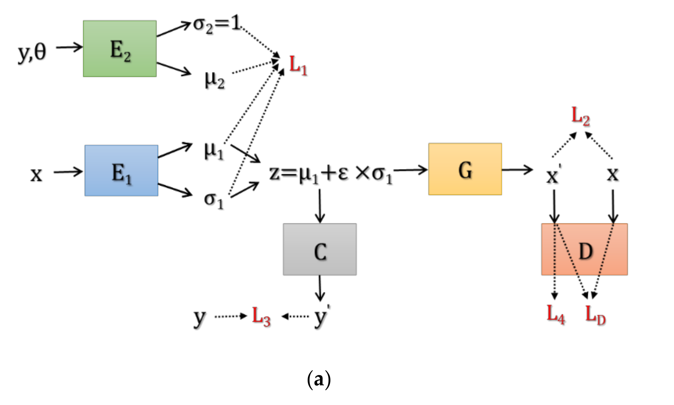
2.3. Network Architecture
Based on the above model, the overall network of the proposed CVAE-GAN is shown in
Figure 2a. It is composed of 5 sub-networks, i.e., the encoder networks
and
, the generation network
, the classification network
and the discrimination network
.
,
,
,
are expected to fit the distributions
and
in Equation (7), respectively. More specifically,
is used to realize the functions of
in
,
is used to realize the function
in
, and
is used to realize the function
in
. The function of condition generation is realized by jointly utilizing the encoder network
and the generation network
. By projecting the images into the feature space with
and generating the images from the features with
, the attributes of the target can be explained in some extent. Besides, by using
and
, we can classify the known classes and recognize the unknown classes.
The particular architectures of the sub-networks used in the experiment section are shown in
Figure 2b.
,
and
are all modified from the popular U-Net [
41] which is widely used in natural image processing.
is constructed by using the multi-layer perceptron. In the figure, Conv denotes a convolution layer, while ConvT means a transposed convolution layer. Conv(
c_in, c_out, k, s, p) indicates the layer who has
c_in input channels,
c_out output channels and a
k ×
k sized convolution filter with stride =
s and padding =
p. Linear(
a_in,
a_out) indicates a full-connection layer with input size
a_in and output size
a_out. BN and DP are the abbreviations of BatchNorm and Dropout.
is not shown in
Figure 2b, which is simply constructed according to (13). The total number of parameters in CVAE-GAN is about 33.46 million.
In the network training, a reparameterization trick [
29] is used to sample
. It aims to make the sampling step derivable, which is expressed as
where
is the noise with the standard normal distribution
,
. Thus, the sampled
has the normal distribution
. The second term in Equation (7) can be expressed in the summation form with the samples of
as
Since the network is usually trained with mini-batch, the sample number for in Equation (15) can be set as for each iteration. Similarly, one sample of is also used for and in Equation (7).
3. Experiments
In this section, the commonly used public MSTAR data set is applied to test the proposed feature learning method. There are 10 types of vehicle targets in the data set, including 2S1 (Self-Propelled Howitzer), BDRM2 (Armored Reconnaissance), BTR60 (Armored Personnel Carrier), D7 (Bulldozer), T62 (Tank), ZIL131 (Military Truck), ZSU234 (Air Defense Unit), T72 (Main Battle Tank), BMP2(Infantry Fighting Vehicle) and BTR70(Armored Personnel Carrier), which are numbered from Class 0 to Class 9 in order. The former 7 classes are selected as the known target classes and the latter 3 classes are the unknown classes. The target images of the 7 known classes with depression angle of are used for training, while the images of all the 10 classes with depression angle of are used for testing. In the training, inputs of the network contain the SAR image, the azimuth angle and the corresponding class label. All the SAR images are cropped to the size of 128 × 128. The azimuth angle information is represented as a 2-D vector , where denotes the azimuth angle. The class labels are encoded into the 7-D one-hot vectors. The dimension of the latent variable is set as 512. The constants in the classifier are set as in the experiment.
In order to make the training of CVAE-GAN easier, a stepwise training strategy is applied. In the first, the loss is utilized to train the CVAE networks , and . Next, the classification network together with the CVAE networks will be trained by using the loss . In the last, the loss and will be trained adversarially to improve the clarity of generated images. The network is initialized with the default parameters in Pytorch and is trained by using the Adam optimization with a learning rate of 0.0001. All the experiments are performed on a workstation with Intel Core i9-9900 CPU and NVIDIA GeForce RTX 2080 Ti GPU.
3.1. Visualization of the Learned Feature Space
The latent variables, i.e., the extracted features, are high-dimensional of 512, which are difficult to visualize. Therefore, the t-distributed stochastic neighbor embedding (t-SNE) [
42], a widely used dimension reduction technique, is utilized to embed the high-dimensional features into a 2-D feature space. Since only the angle of the feature is used for classification in Equation (13), we normalize all the features before visualization.
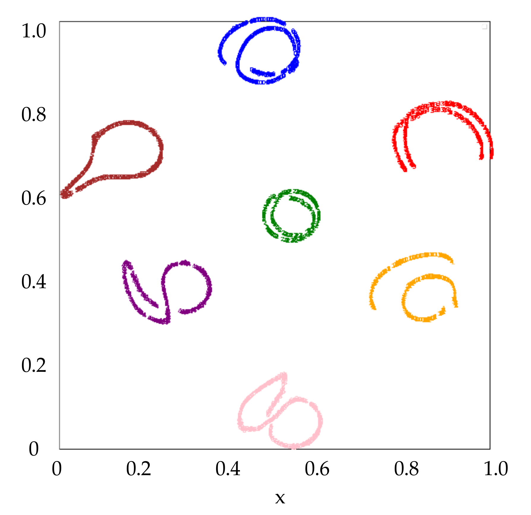
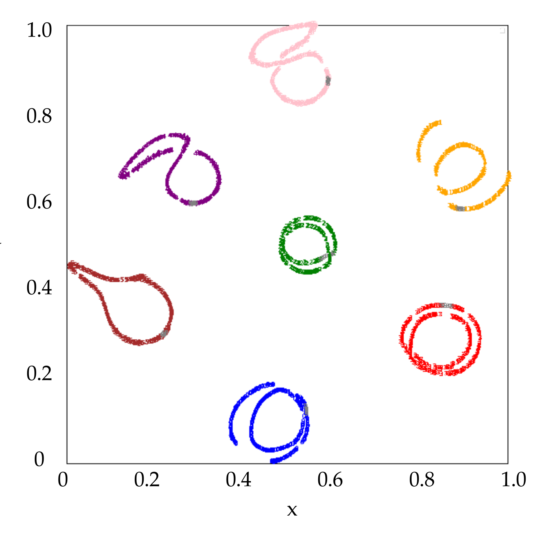
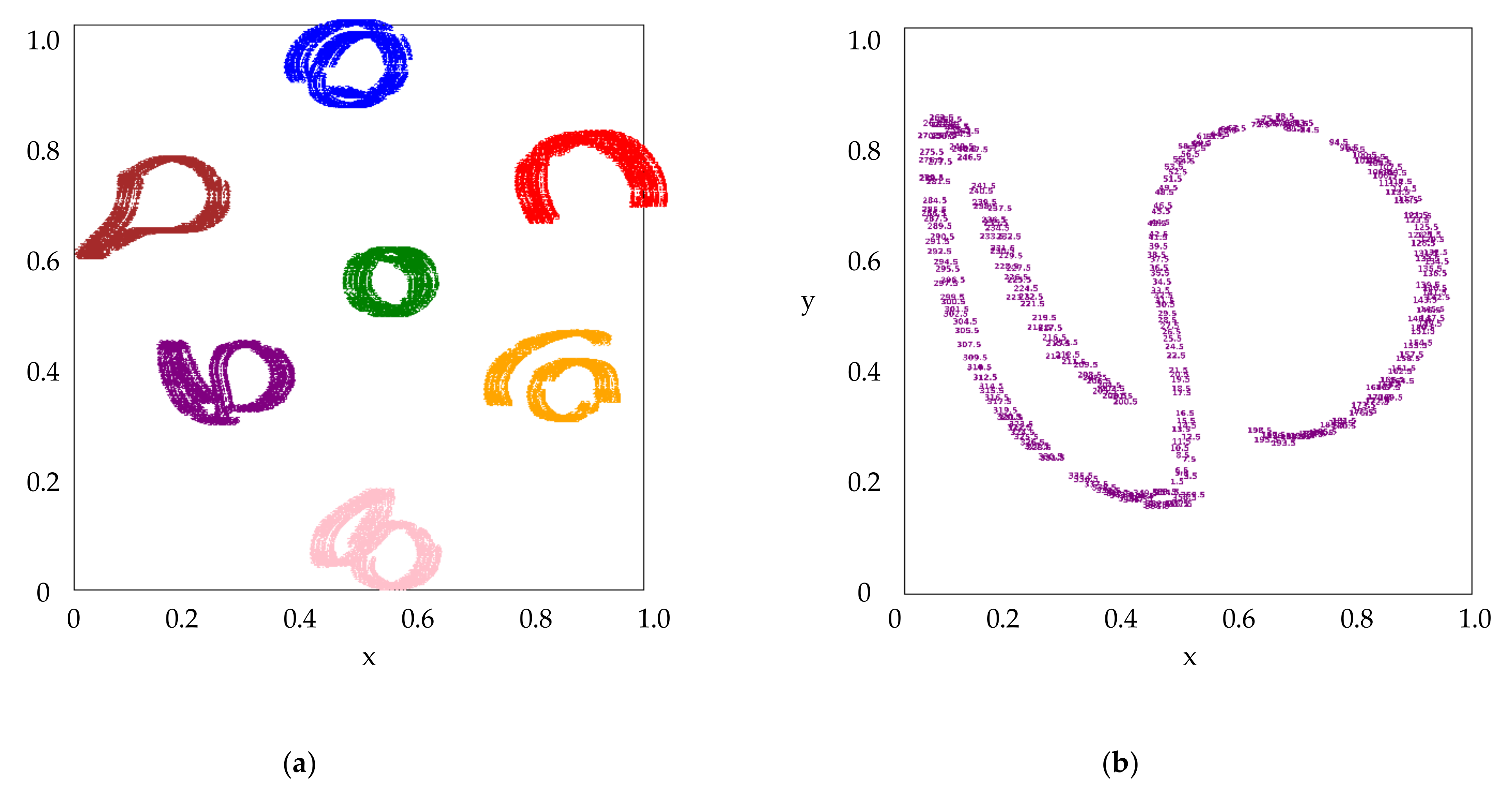
Figure 3 visualizes the extracted features of the 7 known classes with depression angle of
. Colors for Class 0 ~ Class 6 are ‘blue’, ‘orange’, ‘green’, ‘red’, ‘purple’, ‘brown’ and ‘pink’, respectively. It can be seen that different classes can be separated from each other easily in this feature space. The azimuth angles of the features in
Figure 3 are marked in
Figure 4. It shows that the feature of SAR image moves continuously in the space along with the gradual change of azimuth angle. Thus, the extracted feature is useful to explain the angle attribute of the SAR image.
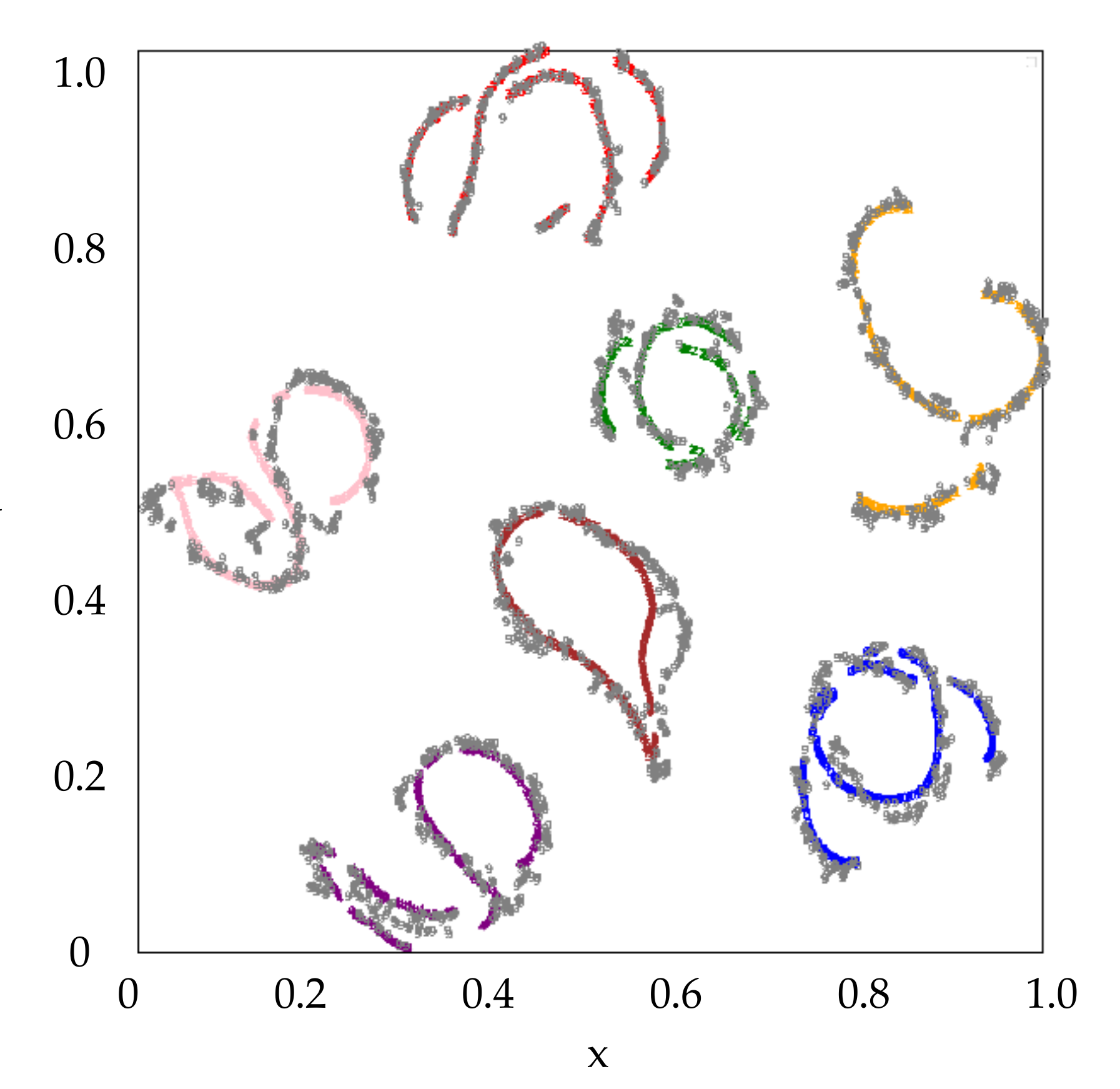
Furthermore, the features of the 7 known classes in the testing data with depression angle of
are also examined. All these extracted features are marked in gray and shown in
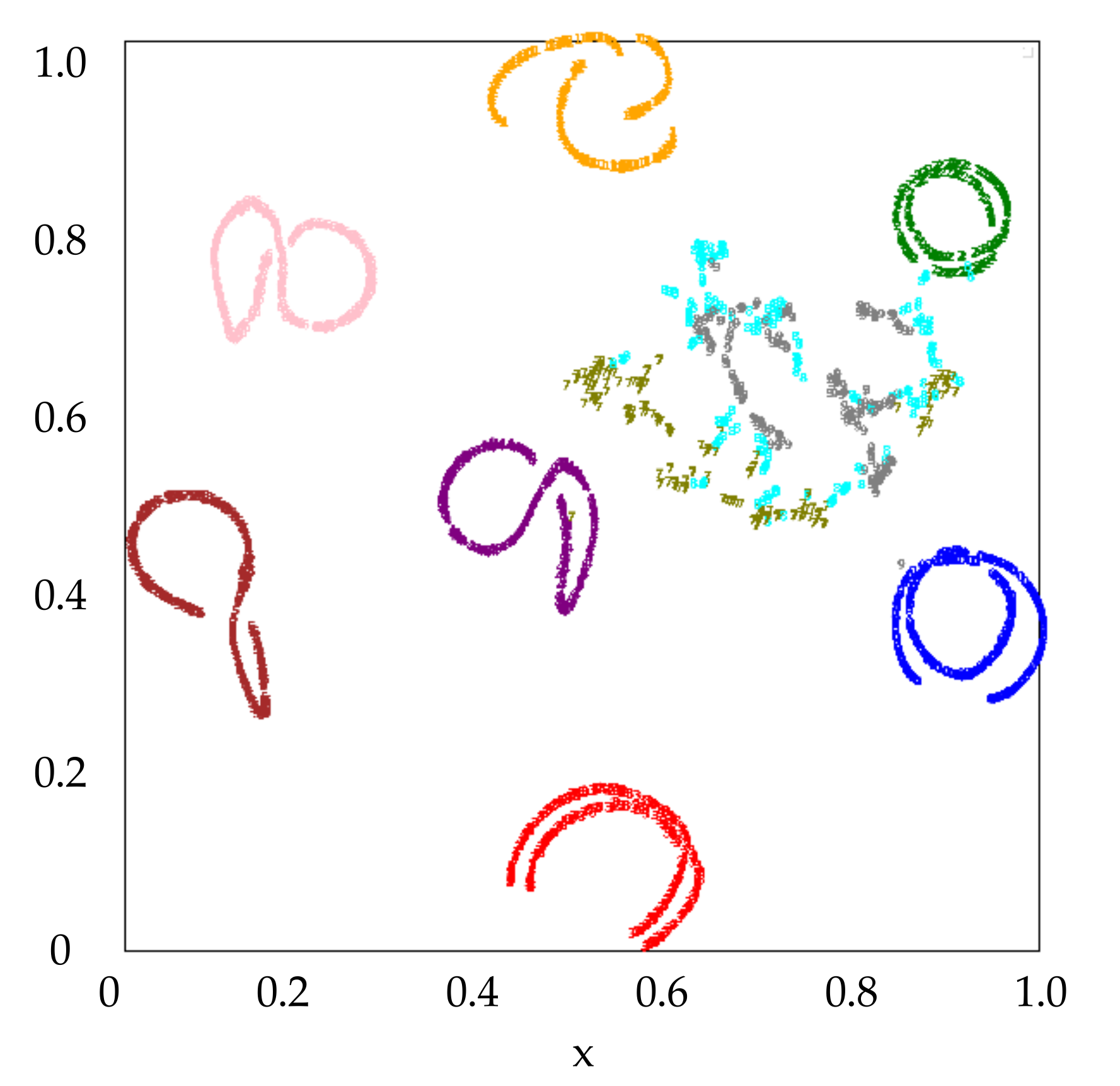
Figure 5. It can be seen the features of the testing data have the similar distribution as that of the training data on the whole. The features of the 3 unknown classes together with the known classes are shown in
Figure 6, where the unknown Class 7, 8 and 9 are marked in ‘olive’, ‘cyan’ and ‘gray’, respectively. We can see most samples of the unknown classes are separated from that of the known classes in the feature space, which makes it possible to distinguish the unknown from the known. We can also see that Class 7 (T72) is close to Class 4 (T62) in the feature space. It indicates that there may be high similarity between the two classes. It is consistent with the physical truth that T72 tank approximates to T62 tank in shape and structure. The analogous conclusion can be made for Class 9 (BTR70) and Class 2 (BTR60). Therefore, the feature space is useful to explain the target attribute of SAR image for the unknown classes.
3.2. Results of Image Generation
In this part, the image generation ability of the proposed model is tested.
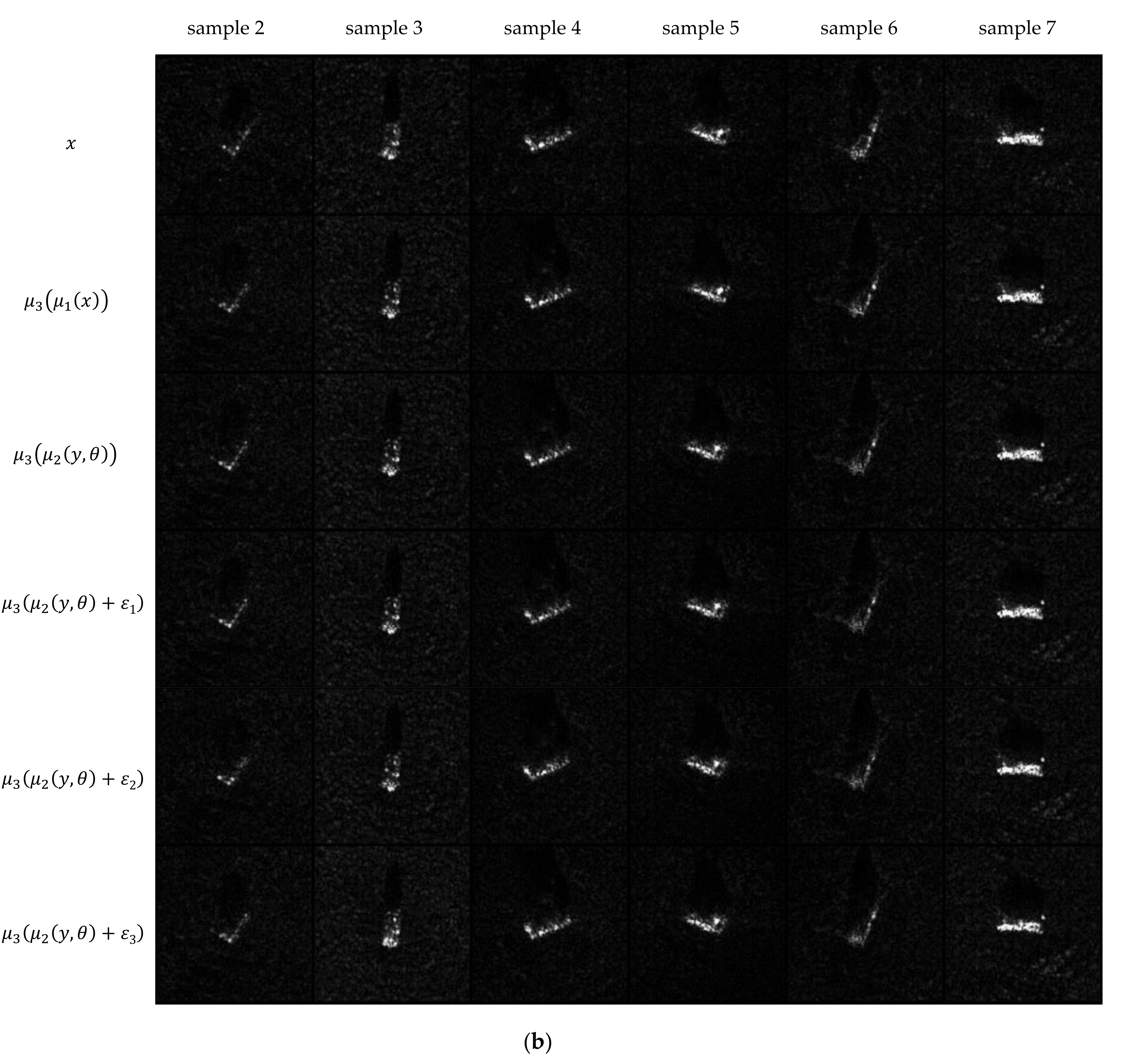
Figure 7 shows the generated images with given conditions.
Figure 7a is the result of one random sample.
is a real SAR image randomly selected from the training data set.
denotes the generated image of
after going through encoding
and decoding
successively. Take the class label
and the azimuth angle
of the real SAR image
, and conduct encoding
and decoding
, we can obtain the conditional generation image
. It can be seen both the encoding-decoding image and the conditional generation image are very similar to the original SAR image. The additive noise is also considered for the conditional generation. The feature now is
, where
is the uniformly distributed noise within the range of
. The noisy images with
are denoted as
,
and
in
Figure 7a. We can see the randomly generated images are still similar to the original images although some slight differences exist. Some other random samples are shown in
Figure 7b, which are consistent with the above result. The normalized features of the noisy images (marked in gray) are visualized in
Figure 8. It demonstrates the generation ability of the continuous feature space.
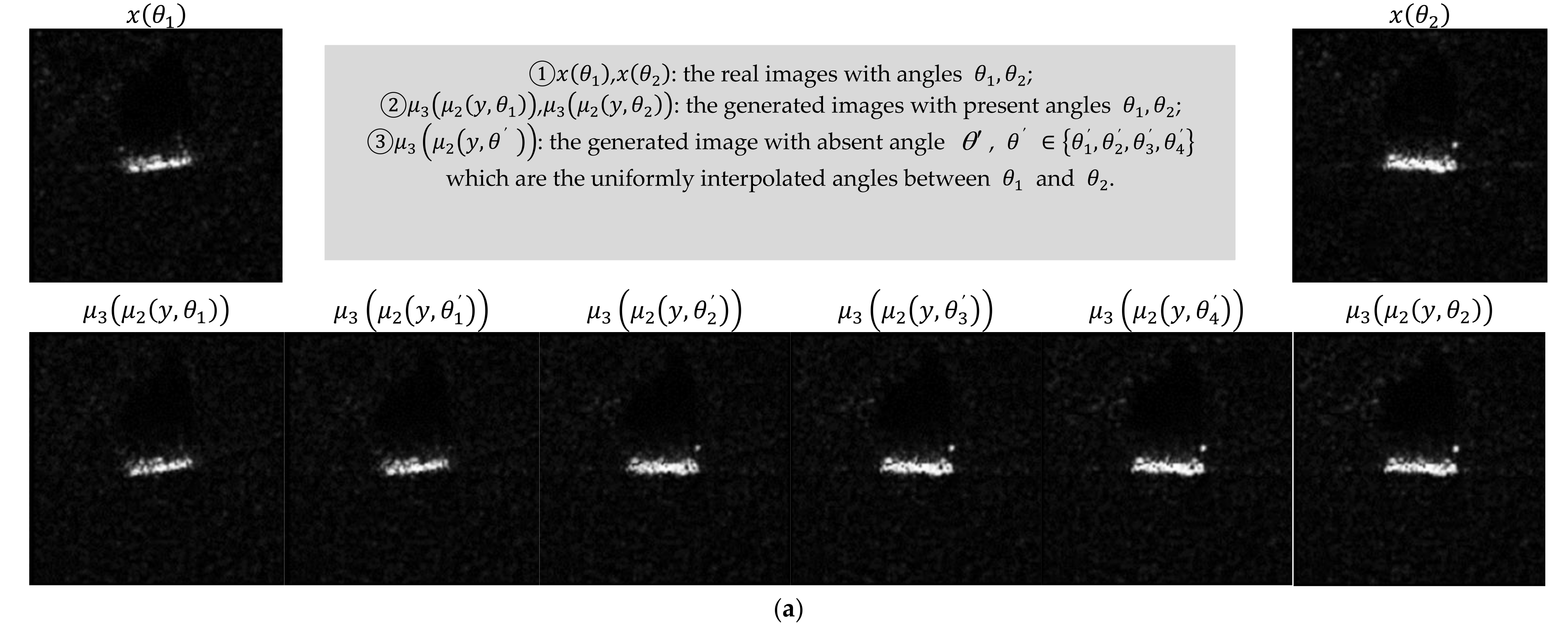
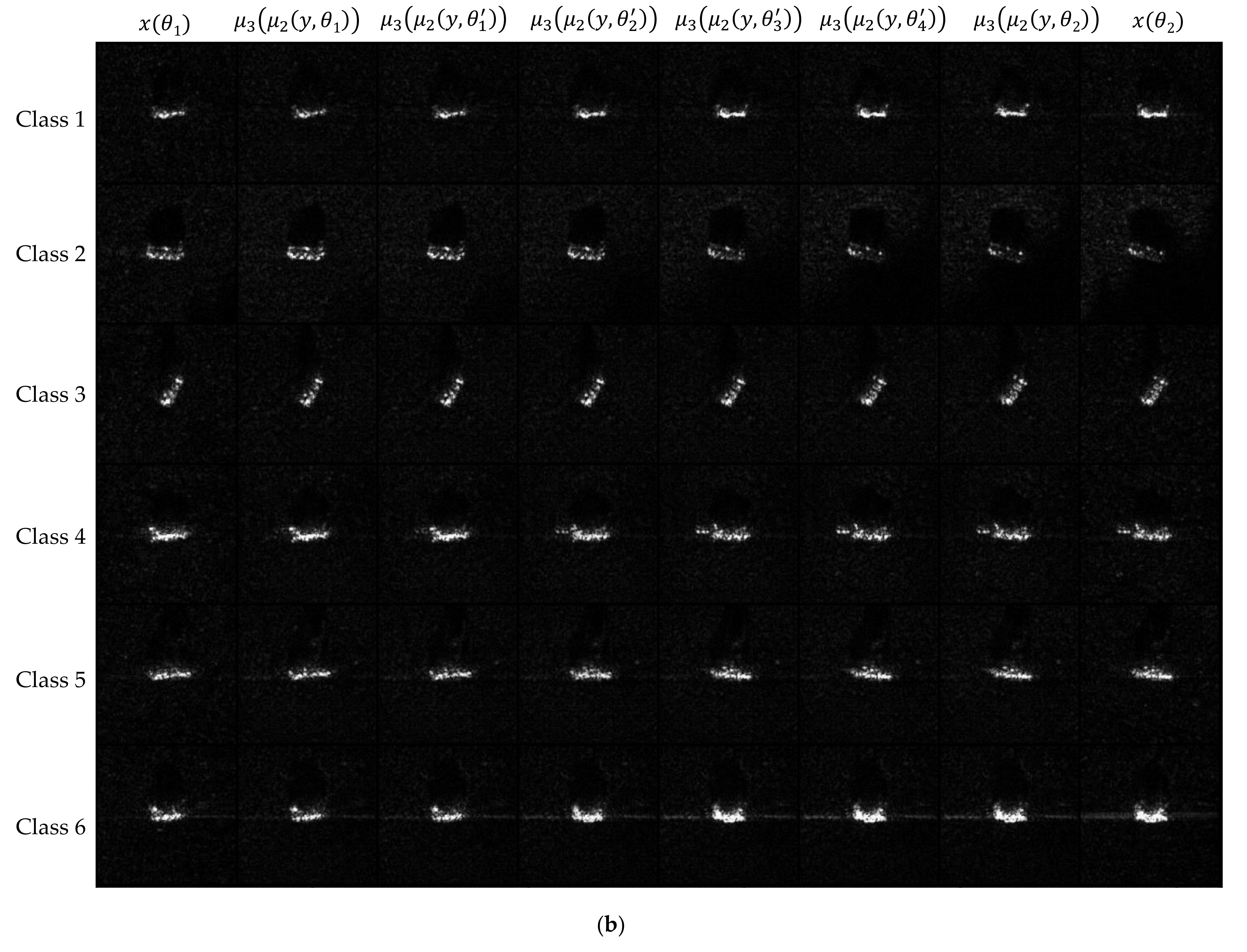
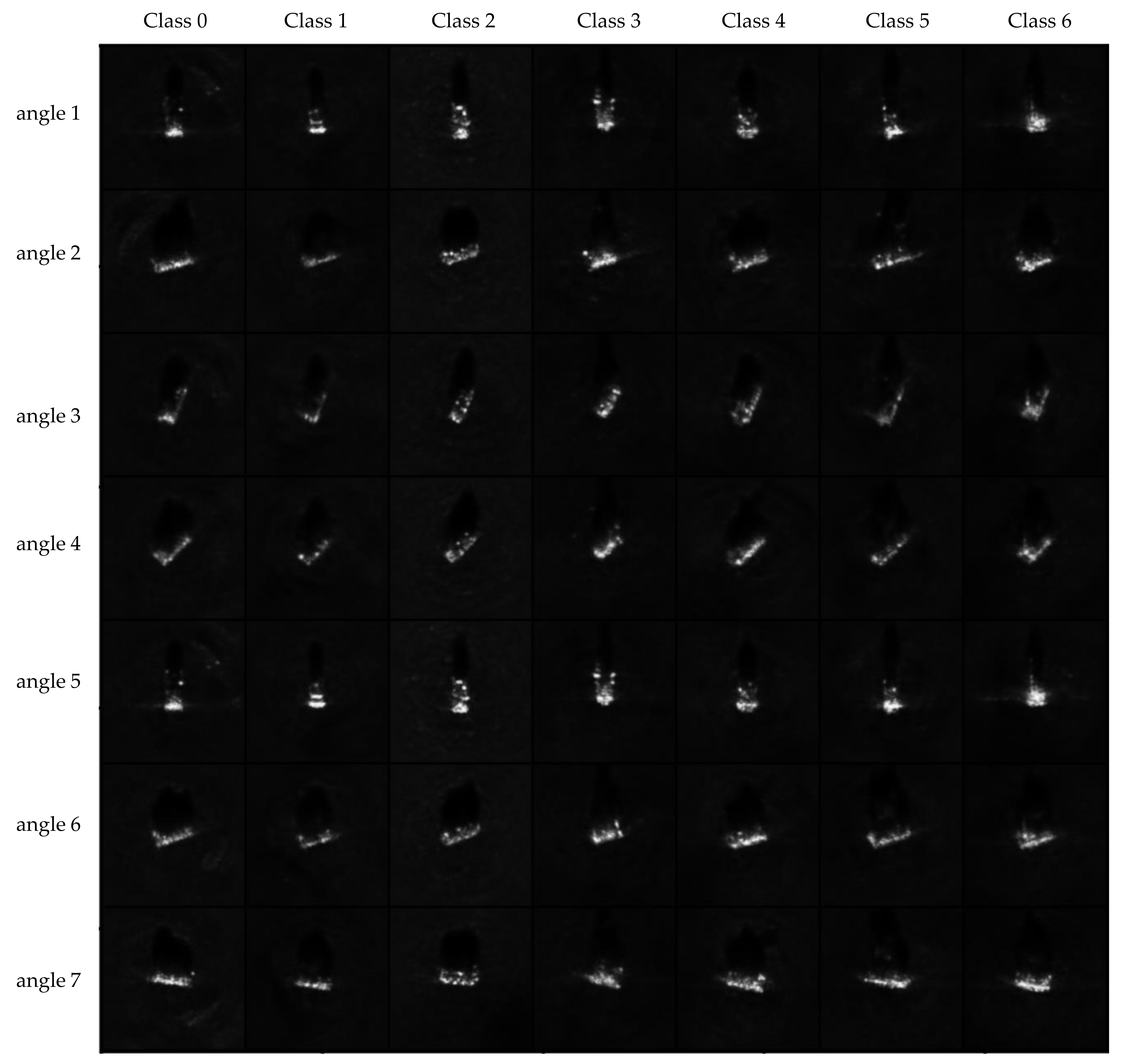
Images with the azimuth angles that are absent in the training data are generated in the following. The obvious angle gaps for Class 0~6 in the training data are (83.3, 93.3), (275.5, 289.5), (200.3, 210.3), (84.5, 94.5), (83.1, 93.1) and (83.0, 93.0), respectively. Sample the angle with equal interval in the gaps and generate the SAR images with the sampled angles and class labels. The results are shown in
Figure 9.
Figure 9a shows the result of Class 0.
and
denote the real images with the angle
,
and
denote the generated images with the present angle
,
denotes the generated image with the absent angle
and
where
are the interpolated absent angles between
and
. The results of Class 1~6 are shown
Figure 9b and the visualized features of the generated images (marked in gray) are shown in
Figure 10. It can be seen the generated images are changed smoothly and can well fill the angle gaps in the feature space.
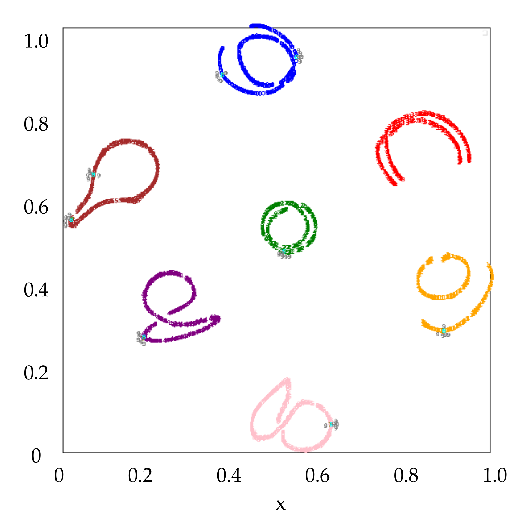
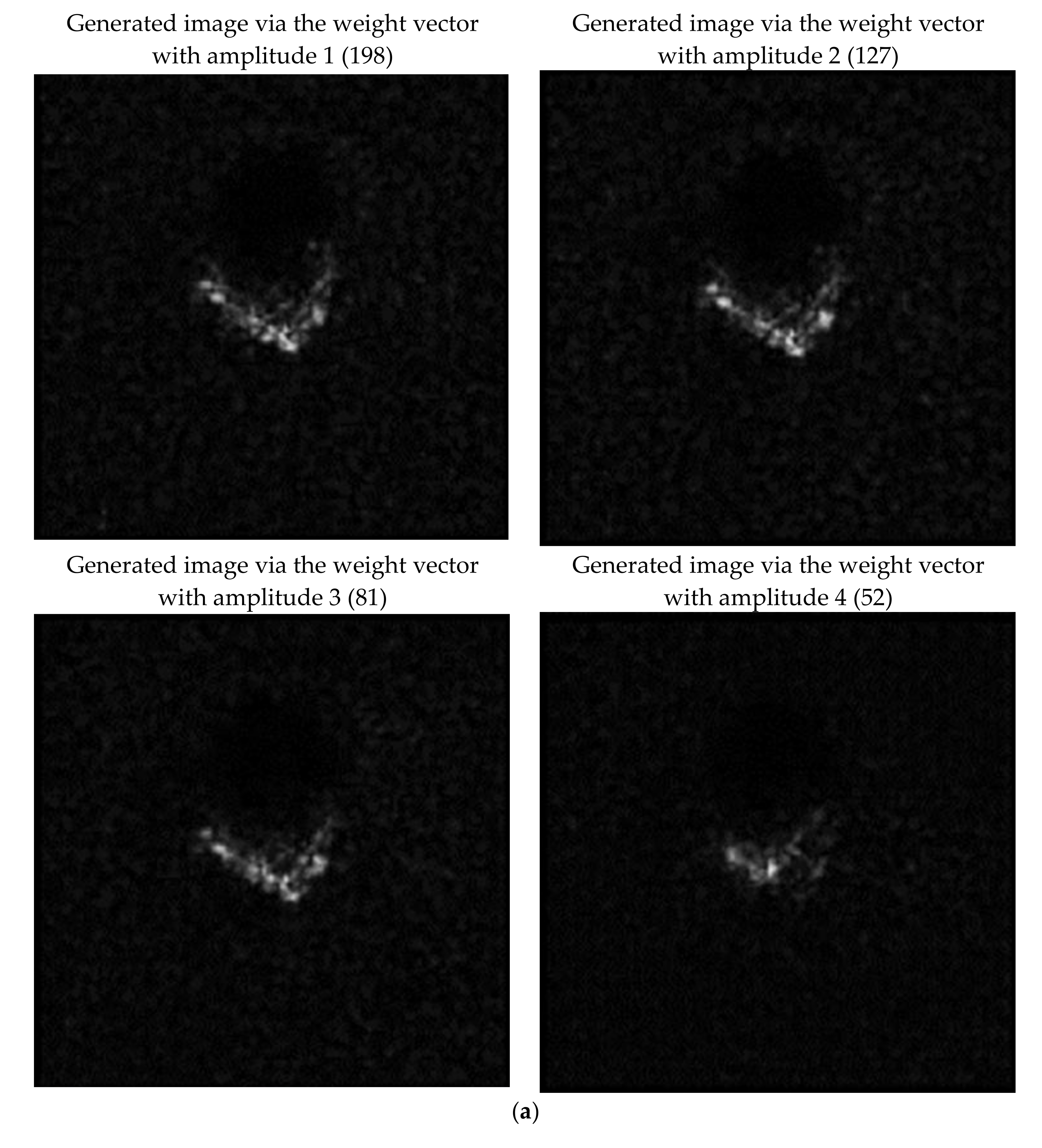
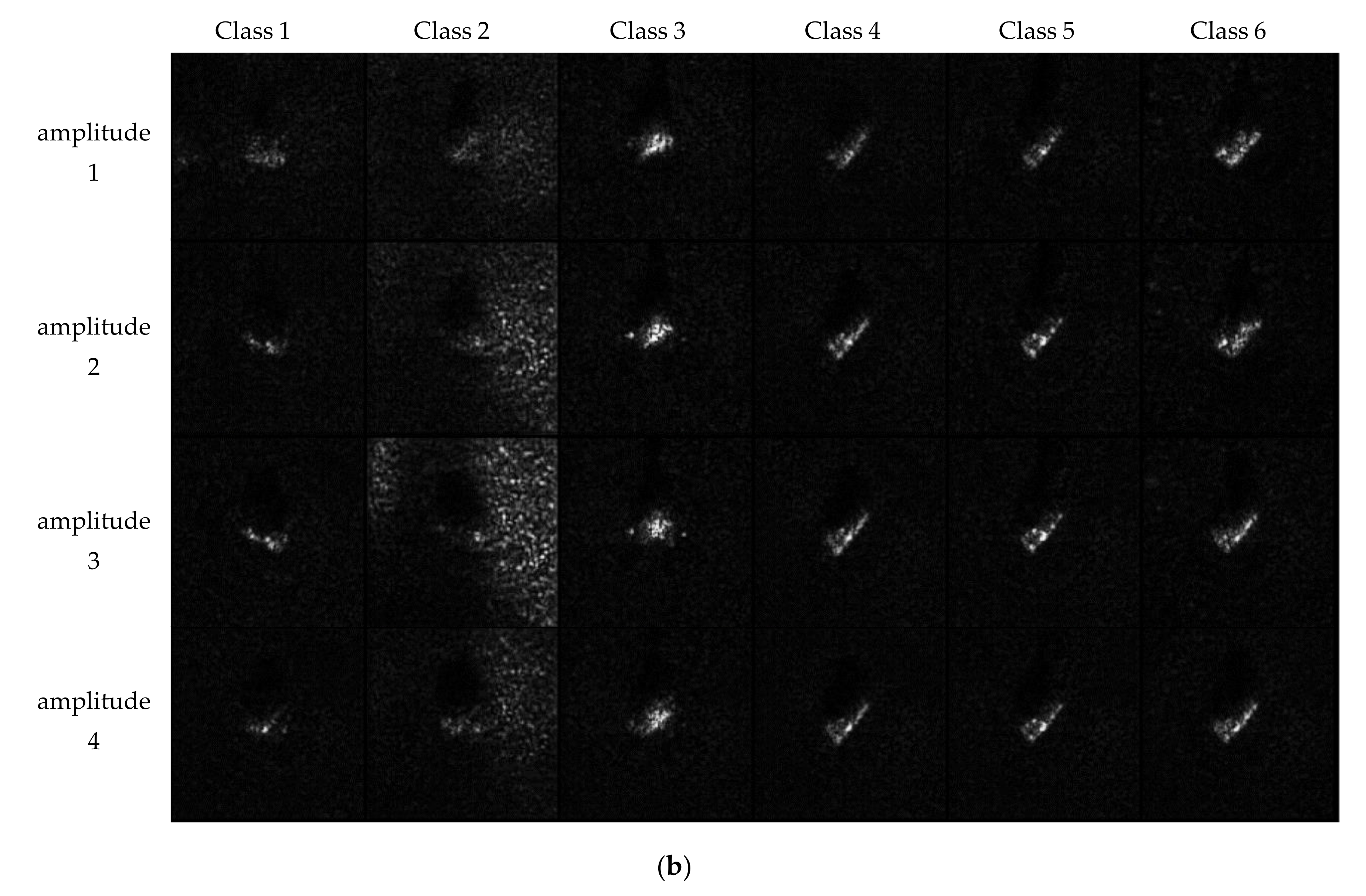
Further, the weight vectors of the classifier for each class are also visualized in the feature space.
Figure 11 shows the result, where the weight vectors are marked as gray ‘9’. We can see the weight vectors are close to features of the samples in the corresponding classes. In the classifier, the images whose features are identical to the weight vectors will obtain the highest classification score for the corresponding class. Next, we will show the generated images by using the weight vectors as features. The feature amplitude may influence the result of the generated image. The mean amplitude of the original weight vectors is about 198 and the mean amplitude of features in the training data is about 70. Herein, we set the weight vectors with different amplitudes of (198, 127, 81, 52). The generated images for Class 0, as an example, are shown individually in
Figure 12a for clarity. The others for Class 1~6 are shown in
Figure 12b. The results may reflect the most recognizable image feature for each class. For example, the generated images for Class 2 all have strong clutter background. It reflects the fact that, in some SAR images for Class 2, the clutter is strong, while for the other classes this characteristic is not obvious. Therefore, for a SAR image who has the strong clutter background, the classifier will classify it into Class 2 with high probability. According to the generated images sampled in the feature space, the actions of the classifier can be understood in some degree.
3.3. Results of SAR Target Recognition with Unknown Classes
In this section, we will test the classification ability of the proposed model on unknown classes. The SAR images with depression angle of
are used for testing. There are 7 known classes with 2049 samples and 3 unknown classes with 698 samples in the test data set. As illustrated in
Figure 1, the target which is located inside the classification boundary will be classified to the corresponding known class (Class 0 ~ Class 6), while the target outside all the classification boundaries of the known classes will be classified to the unknown class. The rate of the samples correctly classified in the known classes is denoted as the true positive ratio (TPR), and the rate of the samples that are falsely classified in the unknown classes is denoted as the false positive ratio (FPR). The classification boundary is adjustable in the test by using a classification threshold
. The recognition results with different
are shown in
Table 1. It can be found, with the increase of
, both TPR and FPR are reduced. The overall accuracy achieves the best result 0.9236 when
.
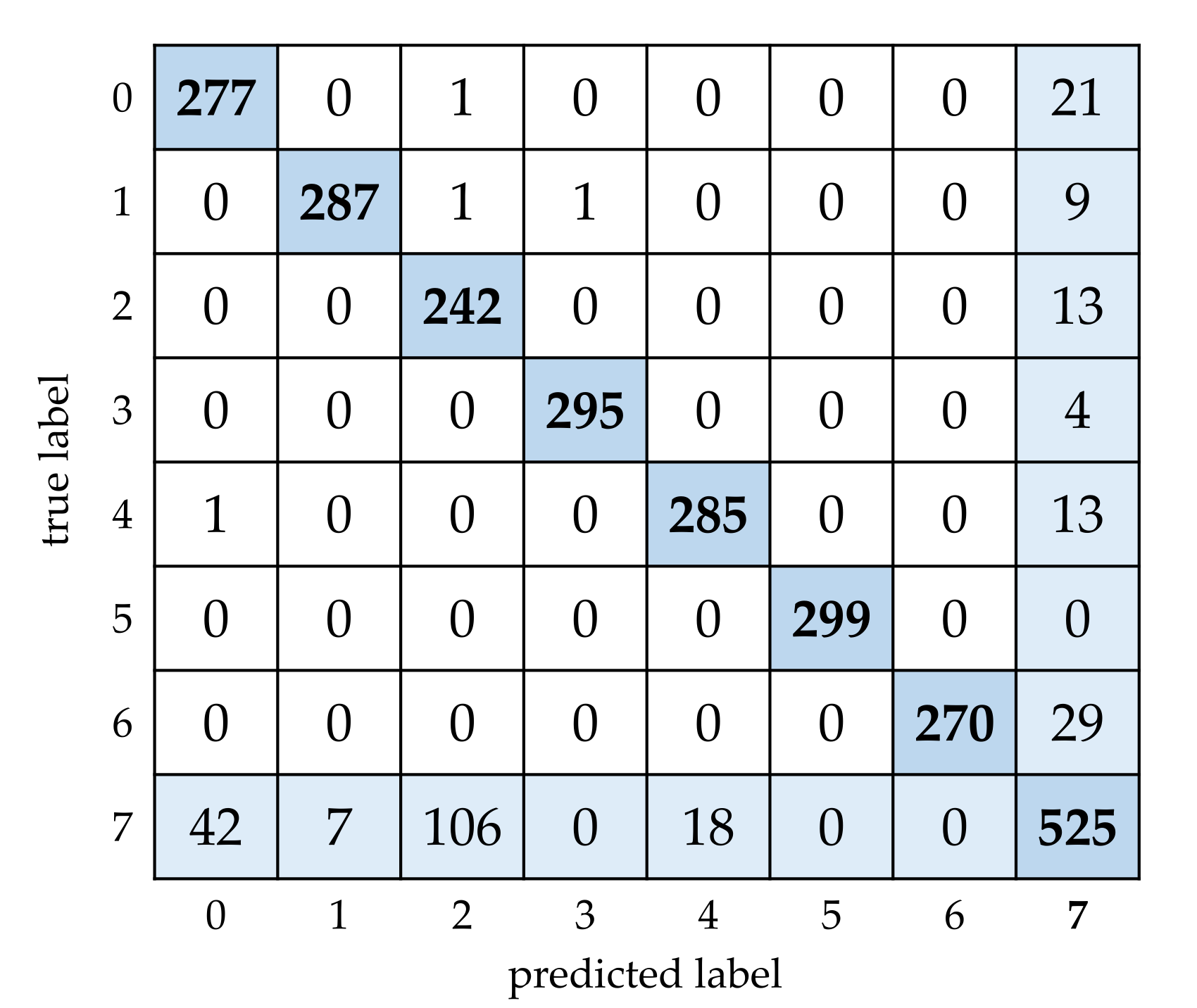
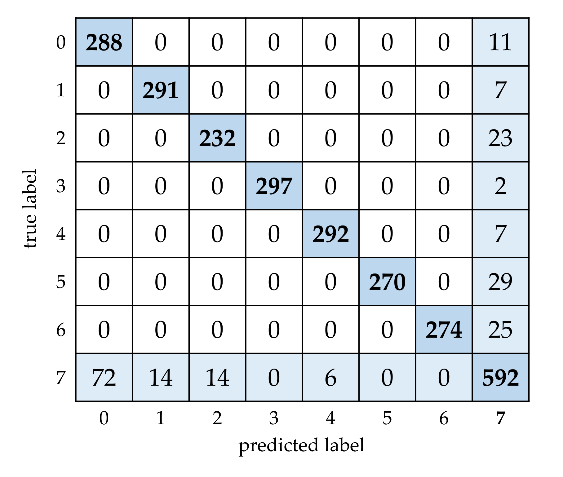
To further illustrate the result, the confusion matrix with
is shown in
Figure 13. It can be seen there are no falsely classified samples among the 7 know classes, but only some falsely classified samples exist between the known and unknown classes. Based on the confusion matrix, the average of precision, recall and F1_score on the 8 classes can be calculated by Equation (16), where
is the total number of classes. The precision, recall and F1_score with
are 0.9410, 0.9359 and 0.9369, respectively.
In the above, the additive angular margin is set as
. The recognition results with different
are also tested, which are shown in
Table 2. We can see all of the accuracy, precision, recall and F1_score are improved with the increase of
. For
and
, the overall accuracy is up to 0.9363. It should be also noted that the network will be hard to convergence as
is too large.
4. Discussion
In this section, we will discuss the above results compared with the existing studies.
With regard to the explainable feature space for unknown SAR target recognition, the related studies have been done in [
23,
24]. The feature spaces built in these papers only represent the categories of the target, but can’t show the other target attributes, such as the azimuth angle, effectively. It can be seen clearly from the Figures 9 and 11 in [
23] and Figures 6 and 7 in [
24]. In this paper, the target attributes including the azimuth angle can be explained in the continuous feature space, which is useful to understand the result of deep network in some extent and benefits for the conditional image generation.
About the image generation, the network proposed in [
23] is able to generate the SAR image with the given class and angle. However, the generated images are blurry as shown in Figures 5 and 7 of [
23]. Besides, some variations of GAN have been proposed to generate the images with given class labels [
43,
44]. Herein, we also test this kind of methods on SAR image generation.
Figure 14 shows the generated SAR images with class labels by using the conditional GAN in [
44]. It can be seen the generated images are clear. However, as well as we know, the conditional GANs only deal with the concrete conditions well, such as the class label, but don’t work for the continuous conditions at present, such as the azimuth angle. Moreover, the conditional VAE, which is without the discriminator compared with the proposed CVAE-GAN, is also tested. The result is shown in
Figure 15. We can see it is able to deal with the continuous angle, but the generated images are not as clear as the conditional GANs. The proposed CVAE-GAN performs well on both the image quality and the conditional generation, as shown in
Figure 7,
Figure 9 and
Figure 12.
With regard to the SAR target recognition with unknown classes, the open set recognition method proposed in [
28] is also tested. The test condition is the same as that in
Section 3.3. The network is built according the
Figure 1 in [
28] and the input images are cropped into the size of 64 × 64 as [
28] did. The network is trained in 300 epochs and all the networks with different epochs are used for the OSR test. The best result is obtained by using the network in epoch 275 and with the threshold 0.1. The confusion matrix is shown in
Figure 16 and the recognition metrics are shown in
Table 3. By comparing with the results in
Section 3.3, we can see the proposed method has the better performance for OSR.


