Article

Laser Scanner–Based Deformation Analysis Using Approximating B-Spline Surfaces

Department of Geodesy and Geoinformation, TU Wien, Wiedner Hauptstr. 8/E120, 1040 Vienna, Austria
*
Author to whom correspondence should be addressed.
Remote Sens. 2021, 13(18), 3551; https://doi.org/10.3390/rs13183551
Submission received: 13 July 2021 / Revised: 18 August 2021 / Accepted: 25 August 2021 / Published: 7 September 2021

Abstract

:
Due to the increased use of areal measurement techniques, such as laser scanning in geodetic monitoring tasks, areal analysis strategies have considerably gained in importance over the last decade. Although a variety of approaches that quasi-continuously model deformations are already proposed in the literature, there are still a multitude of challenges to solve. One of the major interests of engineering geodesy within monitoring tasks is the detection of absolute distortions with respect to a stable reference frame. Determining distortions and simultaneously establishing the joint geodetic datum can be realised by modelling the differences between point clouds acquired in different measuring epochs by means of a rigid body movement that is superimposed by distortions. In a previous study, we discussed the possibility of estimating these rigid body movements from the control points of B-spline surfaces approximating the acquired point clouds. Alternatively, we focus on estimating them by means of constructed points on B-spline surfaces in this study. This strategy has the advantage of larger redundancy compared to the control point–based strategy. Furthermore, the strategy introduced allows for the detection of rigid body movements between point clouds of different epochs and for the simultaneous localisation of areas in which the rigid body movement is superimposed by distortions. The developed approach is based on B-spline models of epoch-wise acquired point clouds, the surface parameters of which define point correspondences on different B-spline surfaces. Using these point correspondences, a RANSAC-approach is used to robustly estimate the parameters of the rigid body movement. The resulting consensus set initially defines the non-distorted areas of the object under investigation, which are extended and statistically verified in a second step. The developed approach is applied to simulated data sets, revealing that distorted areas can be reliably detected and that the parameters of the rigid body movement can be precisely and accurately determined by means of the strategy.

Graphical Abstract

1. Introduction

Geodetic deformation monitoring deals with the measurement, modelling and evaluation of geometric object changes caused by external influences, such as temperature changes, load effects or changes in the groundwater level [1]. Classically, point-based strategies are used to monitor the behaviour of objects over time: By repeatedly measuring signalised characteristic points of the object under investigation, displacement vectors can be derived, representing the object’s deformation [2]. Due to its long tradition in engineering geodesy, sophisticated strategies to analyse point-wise deformation measurements are established. However, point-based deformation analysis also has a variety of drawbacks: In order to represent the behaviour of the entire object of interest by means of single points, characteristic points have to be carefully chosen, often by including prior knowledge of the expected deformation. Regardless of a successful discretisation process, the derived deformation measures are always sparse. Furthermore, the repeated measurement of the same characteristic points requires a signalisation of these points and, thus, access to the object under investigation. Finally, point-based approaches can be very time and labour intensive, especially when large objects are monitored [3,4,5].
The terrestrial laser scanner overcomes these drawbacks of point-based measuring strategies: a laser scanner remotely samples even large objects with a high spatial resolution in a very short time and directly provides a three-dimensional and quasi-continuous description of the object under investigation [3,6,7]. However, despite the metrological strengths of laser scanning, the analysis of the resulting point clouds—especially with regard to a deformation analysis—poses a variety of challenges. Among other things, the measuring principle of laser scanners does not usually allow for the direct reproduction of points in subsequently acquired point clouds [6] and, thus, the direct computation of displacement vectors between different point clouds is not expedient. Furthermore, the single point precision within a laser scanning point cloud may be considerably lower than, for example, the precision of tacheometrically measured signalised points [8]. Nevertheless, numerous strategies to compare point clouds and, thus, to perform a point cloud–based deformation analysis are proposed in the literature. These strategies can be categorised into three classes [6]:
  • When performing a point-to-point (P2P) comparison, it is assumed that point correspondences in different point clouds either exist or can be constructed. Based on these identical points, displacement vectors can be determined. In some situations, the required point correspondences can be established by an appropriate measurement setup (e.g., [9,10]). Alternatively, they can either be constructed by means of local models of at least one of the point clouds (e.g., [11,12]) or by means of feature descriptors (e.g., [13,14]).
  • When implementing a point-to-surface (P2S) comparison, one of the point clouds—usually the point cloud of the first measuring epoch—is approximated by a reference surface. In order to analyse point clouds acquired in subsequent epochs for deformations, the distance with respect to the reference surface is determined for each point of these point clouds. Depending on the type of reference surface chosen, mesh-based approaches (e.g., [15,16]) and approaches based on analytical surfaces (e.g., [12,17]) can be distinguished.
  • When using a surface-to-surface (S2S) comparison, the entirety of the point clouds is modelled either by means of meshes or by means of analytical surfaces. The examination for deformations between these models can be performed in two different ways. The first form of implementation uses the models of the point clouds to generate identical points in the different epochs, allowing for the computation of displacement vectors (e.g., [18,19]). The second form of implementation is based solely on analytical models of the point clouds and compares the estimated parameters of the respective models (e.g., [10,20]).
Strategies using models of point clouds take advantage of the high redundancy in the point clouds in order to overcome the challenge of the comparatively low single point precision within laser scanning point clouds: The theoretical precision of a surface that is determined on the basis of these points is significantly higher than that of the single points [8]. However, two more challenges can be defined when using a model-based analysis approach [21]: Firstly, there is still a lack of interpretable deformation measures between two surfaces. Although displacement vectors fulfil this property, a prerequisite for their use is the correct definition of point correspondences on the surfaces. Secondly, in only a few of the approaches presented in the literature, the deformation’s significance is confirmed by means of statistical tests.
Freeform surfaces, such as B-splines, allow for the modelling of different kinds of objects with various geometric properties. Being parametric surfaces, they directly provide the possibility to define point correspondences on different B-spline surfaces, assuming that the surface parameters are consistently chosen. Moreover, their property of locality allows for the simultaneous modelling of distorted regions of an object and its non-distorted parts by means of one single B-spline surface.
The aim of the present publication is the development of a B-spline-based strategy for performing a point cloud–based deformation analysis, using these beneficial properties of B-splines. Unlike most of the strategies available in the literature, our approach simultaneously determines rigid body movements and distortions of the object under investigation. Being designed as an S2S comparison, all acquired point clouds are modelled by means of consistently parameterised B-spline surfaces, the surface parameters of which are used to define point correspondences. Based on these point correspondences, rigid body movements between the point clouds are estimated, using a robust random sample consensus (RANSAC) approach. The resulting consensus set defines an initial region that is not subjected to additional distortions. In the final step, these stable regions are extended and statistically verified, providing the basis for the computation of displacement vectors in the distorted areas. Both the estimated rigid body movements and the identified distorted regions are confirmed by means of statistical hypothesis testing. Hence, the developed approach combines the strength of areal analysis strategies with the sophisticated tools of the classical point-based deformation analysis.

2. Materials and Methods

2.1. Estimation of Rigid Body Movements and Simultaneous Localisation of Non-Distorted Regions Using Sampled Approximating B-Spline Surfaces

Commonly, the term ‘deformation’ summarises two types of geometric object changes: an object underlying rigid body movements is subject exclusively to rotations and translations, whereas an object underlying distortions changes in shape [1]. The aim of the strategy introduced in the following subsections is to robustly estimate rigid body movements of an object and to simultaneously localise the object’s distorted parts, providing the basis for the determination of displacement vectors.

2.1.1. B-Spline Surfaces for Deformation Analysis

The developed approach is based on approximating B-spline surfaces. The mathematical definition of a B-spline surface is given by the following [22]:
S ^ ( u , v ) = S ^ x ( u , v ) S ^ y ( u , v ) S ^ z ( u , v ) = i = 0 n j = 0 m N i , p ( u ) N j , q ( v ) P i j , 0 u , v 1 .
According to Equation (1), a three-dimensional surface point S ^ ( u , v ) in Cartesian coordinates is computed as the weighted average of ( n + 1 ) · ( m + 1 ) control points P i j . The B-spline basis functions N i , p ( u ) and N i , q ( v ) with degree p and q are the corresponding weights and can be computed recursively (cf. references [23,24]). The basis functions are functions of the surface parameters u and v, locating a surface point on the surface and defining the parameter space. Two knot vectors U = [ u 0 , , u r ] and V = [ v 0 , , v s ] split the B-splines’ domain into knot spans, leading to the B-splines’ property of ‘locality’, meaning that the shifting of a single control point changes the surface only locally.
B-spline surfaces allow for the flexible modelling of a variety of objects under investigation. Hence, they are used in several engineering geodetic applications, either for geometric state descriptions (cf. references [25,26,27]) or in the context of monitoring tasks ([28,29]). In addition to their flexibility, B-spline surfaces have two other properties that qualify them for use within an areal deformation analysis:
  • Firstly, B-spline surfaces are invariant under common geometric transformations, such as the similarity transform: the application of a transformation to the control points P i j of a B-spline surface results in the same surface as the application of this transformation to the surface itself [22]. As proven in [20], the estimated control points of different B-spline surfaces can be used as corresponding points to estimate the parameters of a similarity transform, provided that a joint parameterisation is used when determining the best-fitting B-spline surfaces. However, not only can the control points be used for this purpose, but also surface points S ^ ( u , v ) , with the surface parameters u and v identifying the point correspondences. This property is demonstrated in 
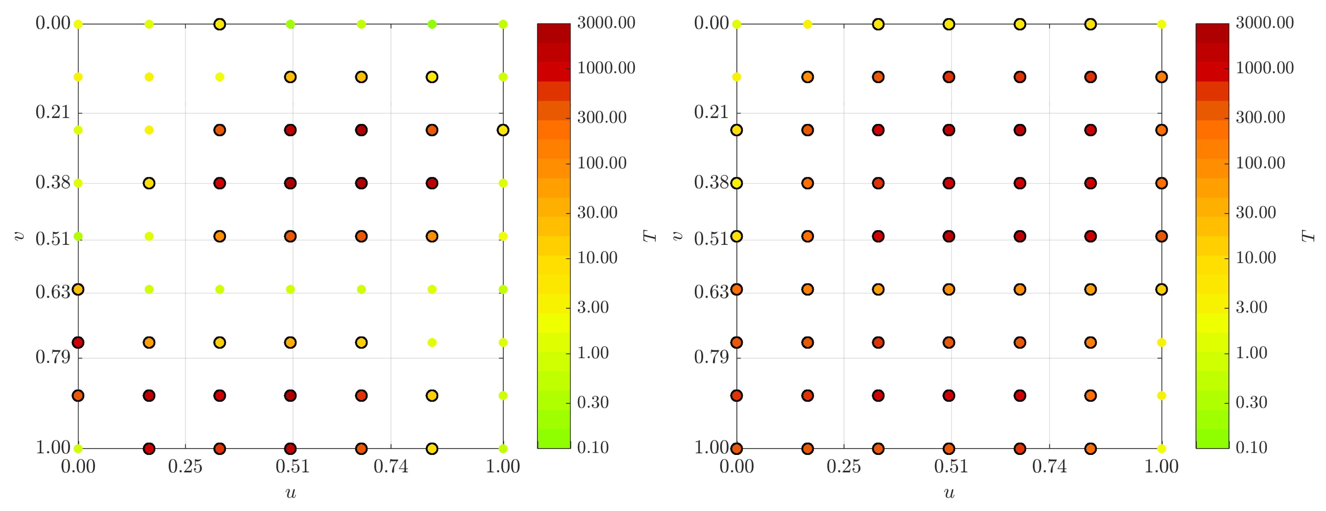
Figure 1, presenting two B-spline surfaces that differ from each other only by rotations and translations (left surface: epoch 1, right surface: epoch 2). As can be seen, parameter grids (green quadrangles) of the surface of epoch 1 that are individually transformed by means of the same transformation parameters as the surface are congruent with the respective grid quadrangles of the transformed surface.
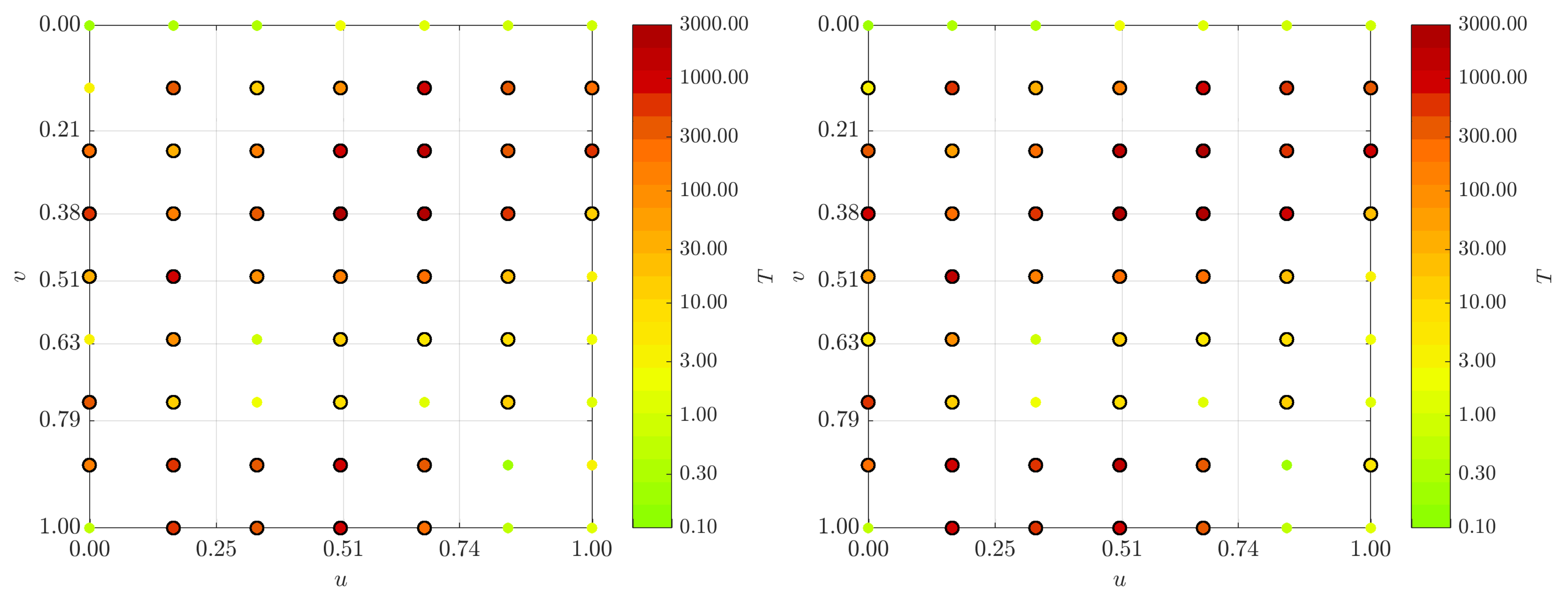
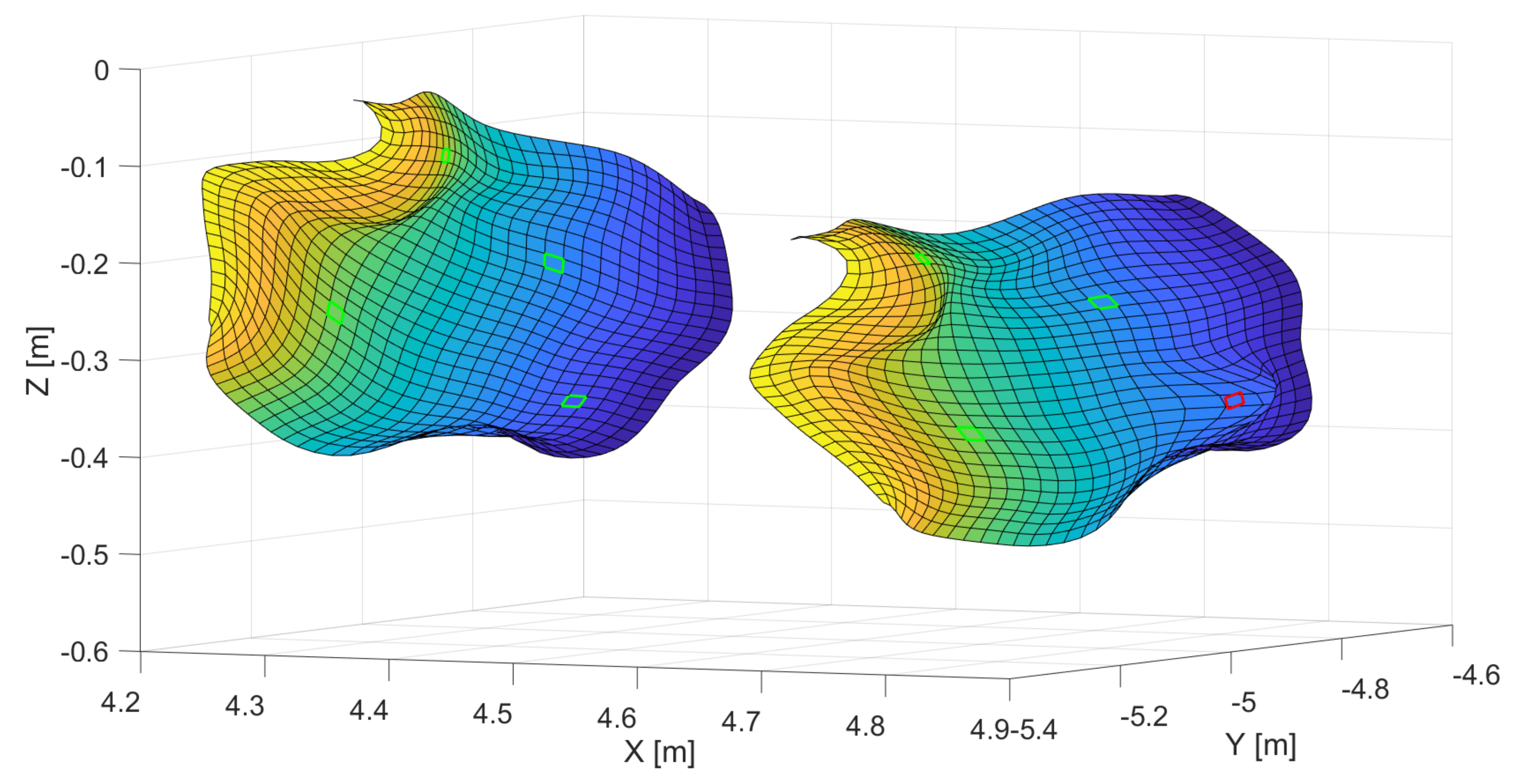
  • Secondly, the locality of the B-spline surfaces directly allows for the modelling and for the localisation of an object’s distortions. For example, when the rigid body movement of a B-spline surface is superimposed by distortions, non-distorted areas can be identified by means of the surface parameter grid as demonstrated in Figure 2. The figure presents two B-spline surfaces that differ from each other by a rigid body movement and a superimposed local distortion (left surface: epoch 1, right surface: epoch 2). The transformation of the four parameter quadrangles (green quadrangles) of the surface of epoch 1, using the same transformation parameters as those for the rigid body movement of the surface, highlights that this local distortion only locally influences the parameter lines: only the red quadrangle in epoch 2—being the only one of the four example quadrangles located in the distorted area—is not congruent with the respective grid quadrangles of the surface of epoch 2.
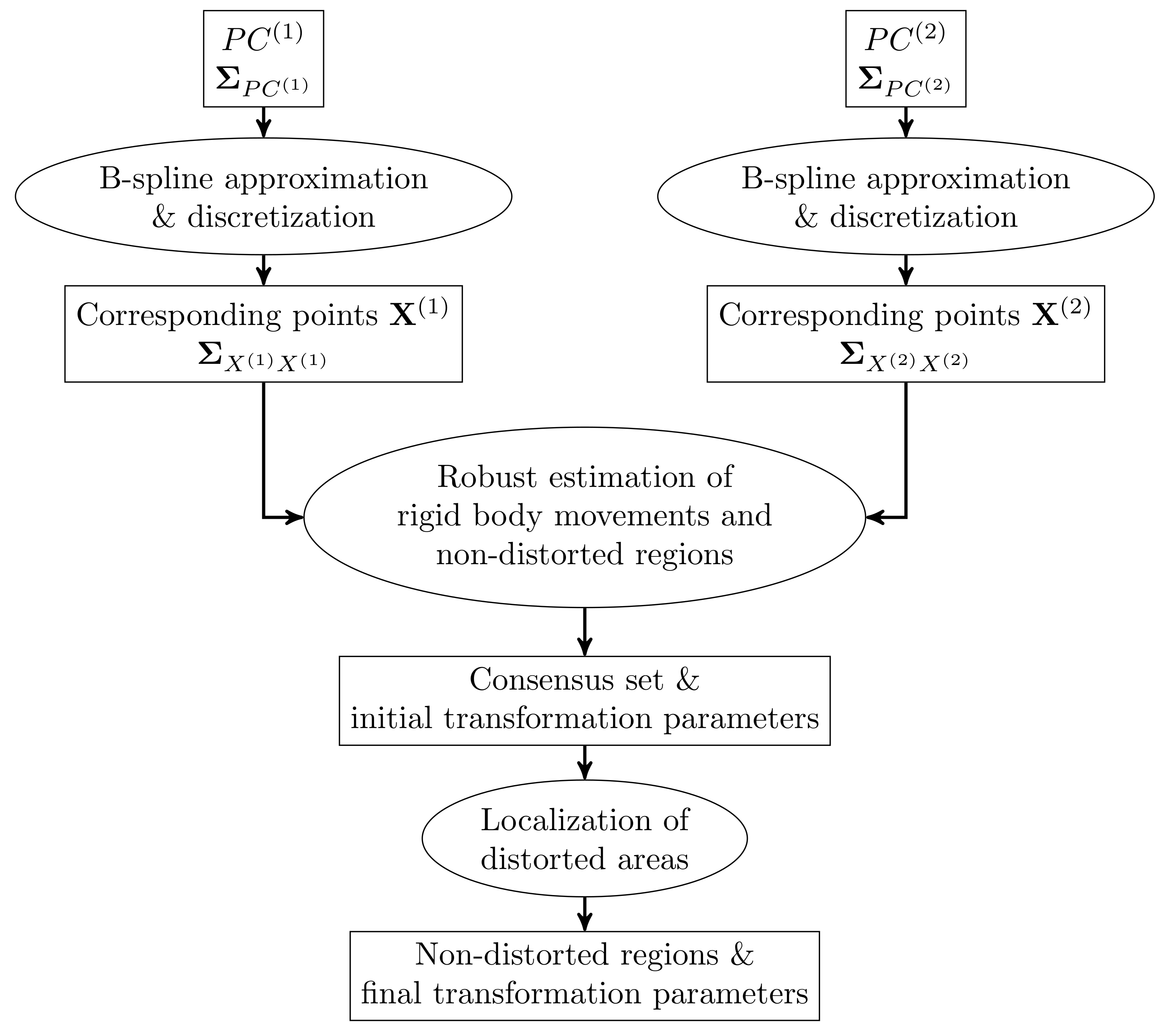
These two properties of B-spline surfaces form the cornerstones of the developed approach that is summarised in the flow chart in Figure 3.
For the sake of simplicity, only two measuring epochs are considered; the extension by further epochs is straightforward.
Starting points are point clouds of an object acquired in two different measuring epochs ( P C ( 1 ) and P C ( 2 ) ), along with their variance covariance matrices (VCM) ( Σ P C ( 1 ) and Σ P C ( 2 ) ). Between these two epochs, the object may undergo rigid body movements, which additionally may be superimposed by distortions. It is assumed, however, that only parts of the object are subject to distortions. The resulting non-distorted regions of the object are necessary for successful application of the developed approach.
Both point clouds are initially approximated by means of best-fitting B-spline surfaces, taking into account the stochastic information of the available point clouds (Section 2.1.2). Due to the use of joint parameterisation during this step, afterwards, the surface parameters can be used to defined point correspondences on the estimated B-spline surfaces. These corresponding points, resulting from discretisations of the B-spline surfaces (Section 2.1.3), are then used to robustly estimate rigid body movements and to initially define non-distorted regions of the object (Section 2.1.4 and Section 2.1.5). Finally, the non-distorted regions are extended and their stability as well as their extents are statistically confirmed (Section 2.1.6).

2.1.2. Point Cloud Modelling by Means of Best-Fitting B-Spline Surfaces

When using B-spline surfaces (cf. Equation (1)) to model a point cloud P C ( i e ) ( i e = 1 , 2 : indicating the measuring epoch), the n l ( i e ) individual points of the point cloud are the observations S k ( i e ) ( u , v ) ( k = 1 , , n l ( i e ) ) that are used to determine the best-fitting B-spline surface S ^ k ( i e ) ( u , v ) :
S ^ k ( i e ) ( u , v ) = S k ( i e ) ( u , v ) + ε k ( i e ) ( u , v ) ,
with the three-dimensional residual vectors ε k ( i e ) ( u , v ) . As in Equation (1), each observation S k ( i e ) ( u , v ) is a three-dimensional point expressed in Cartesian coordinates.
Usually, only the position of the control points P i j (cf. Equation (1), for reasons of simplicity, the epochal affiliations indicated by the superscript ( i e ) are not carried along) is estimated in a linear Gauß Markov model, according to the following [31]:
ϑ ^ P = ( A T · Q ll 1 · A ) 1 A T · Q ll 1 · l .
In Equation (3), the vector of unknowns ϑ ^ P summarises the estimated positions of all ( n + 1 ) · ( m + 1 ) control points and is ordered coordinate-wise. The observation vector l is structured accordingly and contains the observed noisy surface points S k ( u , v ) . The stochastic behaviour of the observations is characterised by the corresponding cofactor matrix Q ll , the inverse of which is used as a weighting matrix in the estimation and which differs from the corresponding VCM by the a priori variance factor σ 0 2 [1]:
Σ ll = σ 0 2 · Q ll .
The design matrix A , describing the functional relationship between observations and unknowns, is determined by means of the B-spline basis functions [31]:
A = N 0 , p ( u 1 ) N 0 , q ( v 1 ) N n , p ( u 1 ) N m , q ( v 1 ) N 0 , p ( u n l ) N 0 , q ( v n l ) N n , p ( u n l ) N m , q ( v n l ) I 3 × 3 ,
with I 3 x 3 being the 3 × 3 identity matrix. The vector of estimated control points ϑ ^ P is completed by the corresponding VCM Σ ϑ ^ ϑ ^ , containing the stochastic information of the estimated control points [1]:
Σ ϑ ^ ϑ ^ = σ ^ 0 2 · ( A T · Q ll 1 · A ) 1 , w i t h σ ^ 0 2 = ε ^ T · Q ll 1 · ε ^ 3 ( n l ( n + 1 ) · ( m + 1 ) )
and with the vector of estimated residuals ε ^ being computed according to the following:
ε ^ = l ^ l = A ϑ ^ P l .
A geometrical interpretation of the estimation l ^ = A ϑ ^ P in Equation (7) is that the original vector of observations l is orthogonally projected to the 3 ( n + 1 ) · ( m + 1 ) -dimensional column space of the design matrix A [32]. Thus, the vector of estimated observations l ^ can be computed as a linear combination of the vector of estimated control points ϑ ^ P . Due to n l > ( n + 1 ) · ( m + 1 ) , linear dependencies between the estimated observations emerge. The corresponding VCM of the vector of estimated observations
Σ l ^ l ^ = A · Σ ϑ ^ ϑ ^ · A T ,
thus, has a maximum rank of r k ( Σ l ^ l ^ ) = 3 ( n + 1 ) · ( m + 1 ) and—assuming an overdetermined estimation problem—is singular.
The strategy described above requires appropriately determining the remaining parameter groups of the best-fitting B-spline surface separately from the adjustment of the optimal control points: The B-spline’s degrees p and q are usually specified a priori. Using cubic B-splines with p = 3 and q = 3 is a generally accepted choice [22]. Strategies to determine the knot vectors are proposed in, for example, [22,31,33]. The optimal number of control points to be estimated can be interpreted as a model selection problem and can either be solved by classical model selection strategies or by structural risk minimisation (cf. [34,35]). The latter strategy has the advantage that the degrees p and q can also be taken into account during model selection, rather than choosing them arbitrarily [36]. Finally, appropriate surface parameters u and v have to be allocated to the observations (cf. e.g., [37] for an iterative parameterisation approach for laser scanning point clouds). When B-spline surfaces are used as a basis for deformation analysis, however, an independent parameterisation of different point clouds is not expedient; rather, a joint parameterisation has to be implemented as demonstrated in [35]. As simulated data sets are investigated in this initial study (cf. Section 2.2), nominal values for degrees, knot vectors and surface parameters are available and, therefore, the appropriate determination of these parameter groups can be left aside during this initial study.

2.1.3. Constructing Identical Points on Approximating B-Spline Surfaces

Having estimated the best-fitting B-spline surfaces, they are used to construct n i d = n i d , u · n i d , v identical (id) points X k , l ( i e ) in the two measuring epochs i e = 1 and i e = 2 . Provided that the surfaces are based on a joint parameterisation, the surface parameters u and v, discretising the estimated surfaces (cf. Equations (1) and (2)), can be used for this purpose:
X k , l ( i e ) = S ^ ( i e ) ( u k , v l ) , w i t h   k = 1 , . . . , n i d , u , l = 1 , . . . , n i d , v a n d   i e = 1 , 2 .
Using the stochastic information of the estimated control points, the sampled surface points are completed by their VCMs Σ X ( i e ) , X ( i e ) . Following the considerations in Section 2.1.2, linear dependencies emerge between the discretised points as soon as n i d > ( n + 1 ) · ( m + 1 ) , resulting in rank defects of the corresponding VCMs Σ X ( i e ) , X ( i e ) . More precisely, a rank defect occurs in at least one parameter direction of the B-spline surface when the number of discretised surface points exceeds the number of estimated control points. The rank defect linked to the u-direction, therefore, can be computed according to the following [30]:
δ u = 0 if n i d , u n + 1 3 · ( n i d , u ( n + 1 ) ) ( m + 1 ) o t h e r w i s e ,
and the rank defect linked to the v-direction accordingly arises to the following:
δ v = 0 if n i d , v m + 1 3 · ( n i d , v ( m + 1 ) ) ( n + 1 ) o t h e r w i s e .
The overall rank defect δ is the sum of these two parts [30]:
δ = δ u + δ v .
This singularity in the VCMs of the corresponding points represents an important difference to deformation models in which the observed data points are directly incorporated.

2.1.4. Estimation of Rigid Body Movements

The estimation of rigid body movements of an object of interest is based on n i d three-dimensional corresponding points X k , l ( 1 ) and X k , l ( 2 ) ( k = 1 , , n i d , u , l = 1 , , n i d , v ) in two measuring epochs, in this study on corresponding surface points (cf. Equation (9)).
Assuming that the object undergoes solely rigid body movements, all corresponding points—just like the entire surface—are subject to translations (summarised in the translation vector t ) and rotations (fully described by means of the rotation matrix R , containing the rotation angles ω , ϕ and κ ). Sometimes, a change of scale (indicated by the scale factor s) is also included, resulting in the mathematical formulation of a three-dimensional similarity transform [1]:
X k , l ( 2 ) = s · R · X k , l ( 1 ) + t , k = 1 , , n i d , u , l = 1 , , n i d , v .
When estimating the parameters of the similarity transform t , R and s based on the corresponding surface points, it must be taken into account that both the points X k , l ( 1 ) available in the start system and the points X k , l ( 2 ) available in the target system are defined by estimated B-spline surfaces and, thus, are subject to uncertainties. In order to include the stochastic information of both point groups into the estimation of the transformation parameters, two strategies, delivering identical results, exist [38]: Either the transformation parameters are estimated in a Gauß–Helmert model, or the classical Gauß–Markov model, assuming the points in the start system to be deterministic, is extended. Because of the easier possibility to extend the approach to a robust one, the second variant is chosen here [30].
Assuming that the data sets under investigation are acquired by means of the same laser scanner and, hence, neglecting the scale factor s, the extended functional model to estimate the transformation parameters is then given by the following [38]:
X ^ k , l ( 2 ) = X k , l ( 2 ) + e k , l ( 2 ) = R · X k , l * ( 1 ) + t
X ^ k , l ( 1 ) = X k , l ( 1 ) + e k , l ( 1 ) = X k , l * ( 1 ) ,
with e k , l ( i e ) ( i e = 1 , 2 ) being residual vectors. The first part of the model (Equation (14)) describes the functional relationship between the identical points in the two epochs by means of the unknown transformation parameters. Equation (15) simultaneously introduces the coordinates of the identical points in the start system as additional observations and, thus, allows for the consideration of their stochastic information. The link between Equations (14) and (15) is given by the estimated point coordinates available in the start system, which are introduced in both equations and are marked with an asterisk. Neglecting inter-epochal correlations, the extended stochastic model is composed of the VCMs Σ X ( 1 ) X ( 1 ) as well as Σ X ( 2 ) X ( 2 ) of the constructed surface points, resulting in the following [38]:
Σ l l = Σ X ( 2 ) X ( 2 ) 0 0 Σ X ( 1 ) X ( 1 ) = σ 0 2 · Q ll .
Based on the functional model in Equations (14) and (15) as well as on the stochastic model in Equation (16), the unknown transformation parameters can be estimated in a non-linear Gauß–Markov model (cf. [38] for more information).

2.1.5. Robust Estimation of Rigid Body Movements

The derivations in Section 2.1.4 are based on the assumption that the object under investigation is only subject to rigid body movements. However, rigid body movements are usually superimposed by additional distortions in reality. When taking into account points that are subject to both rigid body movements and distortions in the estimation of the rigid body movement, these points falsify the estimated transformation parameters. As a consequence, the determination of transformation parameters must necessarily be accompanied by an elimination of surface points in distorted areas. Otherwise, the required congruence of identical points is not given.
Considering points that are subject to both rigid body movements and distortion to be outliers in the context of the similarity transform is one possible strategy to cope with this challenge [30]. In order to accurately estimate rigid body movements in this situation, a robust strategy based on the random sample consensus (RANSAC)-algorithm [39] is proposed in this section. In general, RANSAC is an easy-to-implement method and is characterised by a high breakpoint (>50%). Furthermore, with respect to the presented problem, RANSAC allows for the robust estimation of rigid body movements while obtaining initial information about non-distorted regions.
The general idea of RANSAC is to initially determine the unknown parameters of a model describing n l data points by the minimum number n s u b of data points that is needed for this determination [39]. These n s u b data points are randomly drawn from the entire set of data points. After having computed the model parameters by means of these n s u b points, the distances of the resulting preliminary model to the entirety of the data points are calculated. Points with distances that are within a predefined error tolerance ϵ are considered to be consistent with the determined model parameters. These points form the consensus set S C S . The procedure is repeated iteratively until either the number of points in the consensus set equals a specified minimum number n m i n or a maximum number of iterations i m a x is performed. Finally, the points in the largest consensus set are used to estimate the optimal model parameters.
RANSAC can be directly applied to the robust estimation of rigid body movements that are superimposed by distortions (see Figure 4 for a schematic sketch of the procedure): the six parameters of a three-dimensional similarity transform with neglected scale factor (cf. Equation (14)) can principally be determined by means of two pairs of three-dimensional corresponding data points. However, the estimation of the transformation parameters described in Section 2.1.4 is a non-linear estimation problem and, thus, requires approximate values. As these approximate values are determined by means of quaternions (see, for example, [40]) in this study, a strategy that also yields the scale factor s, the number of point pairs required is n s u b = 3 . Hence, three pairs of sampled surface points are repeatedly and randomly drawn from the entirety of surface points and are afterwards used to determine approximate parameters t 0 , R 0 and s 0 by means of a quaternion approach. (Strictly speaking, the modelled transformation is not a rigid body movement in this step. However, as the results are only approximate values for the final estimation of rigid body movements, this strategy is not to be regarded as critical.) Unlike the quaternion approach, the strategy presented in Section 2.1.4 allows for the accuracies of the corresponding points to be taken into account when estimating rigid body movements. For this reason, the approximate parameters are improved in a second step as described above, yielding optimal translations t ^ 0 and optimal rotations R ^ 0 , describing the rigid body movements of the three chosen surface points. During this step, the scale factor is set to s ^ = 1 [30]. The entirety of computed surface points of the first measuring epoch X k , l ( 1 ) is afterwards transformed using the estimated transformation parameters as follows:
X t r , k , l ( 1 ) = R ^ 0 · X k , l ( 1 ) + t ^ 0 , k = 1 , , n i d , u l = 1 , , n i d , v .
The Euclidean distance
d k , l = | | X t r , k , l ( 1 ) X k , l ( 2 ) | |
between each transformed point X t r , k , l ( 1 ) belonging to epoch E 1 and its corresponding point X k , l ( 2 ) belonging to epoch E 2 provides the basis for the decision of whether a surface point is included in the consensus set of model-conforming points. This distance is compared to the error tolerance as follows:
ϵ k , l = τ · σ d k , l
which is determined by the accuracy σ d k , l of the computed distance d k , l , arising from variance covariance propagation as well as a factor τ , which needs to be chosen appropriately (see below). According to Equation (19), the error tolerance is assessed for each point pair individually since the discretised surface points are not available with a homogeneous precision [30]. When
d k , l ϵ k , l
is fulfilled, the corresponding point pair is assigned to the consensus set S C S .
This procedure is repeated either until the number n C S of points fulfilling Equation (20) is larger than or equal the minimum size n m i n of the consensus set or until the maximum number of iterations i m a x is reached. It is worth noting that it is not possible to distinguish distortions from gross errors in the data during this step. For this reason, it is essential to successfully remove gross errors a priori using standard techniques, for example, when estimating best-fitting B-spline surfaces.
The successful application of the developed strategy requires the definition of three parameters:
  • The parameter τ in Equation (19) has to be chosen in such a way that only model-compliant points are included in S C S . When τ is chosen too small, points will be erroneously identified as outliers, whereas when τ is chosen too large, outliers may be included in the consensus set and, thus, the estimation result will become biased. The influence of the parameter τ on the results is investigated in Section 3.2.
  • The minimum number n m i n of model-compliant points required to accept the current S C S is estimated from the expected amount of gross errors n e r r ( 0 n e r r 1 ) contained in the data set. When n e r r is known, the optimal n m i n can be determined according to the following [41]:
    n m i n = ( 1 n e r r ) · n i d .
  • The maximum number of iterations i m a x is determined by the desired probability P that a solution without outliers is found [41]:
    i m a x = log ( 1 P ) log ( 1 ( 1 n e r r ) n s u b ) .
Finally, after the iteration is completed, the point pairs of the largest consensus set are used to estimate the transformation parameters t ^ C S and R ^ C S in the extended Gauß–Markov model (14) and (15).
With a final statistical global test, comparing the respective a priori variance factor σ 0 2 with the corresponding a posteriori variance factor σ ^ 0 2 , the presence of outliers can be excluded with a confidence probability of 1 α G , with α G being the error probability [42]:
N u l l   h y p o t h e s i s   H 0 , G : E { σ ^ 0 2 } = σ 0 2
A l t e r n a t i v e   h y p o t h e s i s   H A , G : E { σ ^ 0 2 } > σ 0 2 .
The corresponding test variable T G is F-distributed with the degrees of freedom f and :
T G = σ ^ 0 2 σ 0 2   F f , .
If T G lies outside the associated quantile and, thus, the null hypothesis (23) has to be rejected, a further RANSAC iteration should be performed [30]. (It is worth noting that in this formulation of the global test the presence of errors in the stochastic model is excluded).

2.1.6. Statistically Based Localisation of Distortions

Having successfully conducted the steps described in the previous section, estimated parameters of the rigid body movement as well as a consensus set S C S are available. The latter is a set of n C S point pairs that is free from outliers w.r.t to the estimated rigid body movement with the confidence probability of the global test 1 α G . Therefore, these points can already be assigned to the non-distorted region. However, depending on the parameter τ to be chosen, the consensus set does usually not cover the entire non-distorted region of the B-spline surface. Hence, no exact statement can be made about the position and the extent of the distorted regions. Therefore, the consensus set is stepwise and statistically ensured extended by individual point pairs. With the extended consensus set, the parameters of the rigid body movement can be estimated with a higher redundancy and, thus, more precisely.
The starting point of the localisation is the set S T of points to be tested, which includes all data points that are not assigned to the consensus set at the beginning. Using a forward strategy (see below for information about the order in which the points are considered), these points are then sequentially added to the group of points that is already detected as non-distorted. Based on this extended set, the parameters of the rigid body movement are re-estimated. Point pairs that are detected as outliers within this re-estimation are assigned to the distorted region of the surface, whereas points that do not significantly change the estimated transformation parameters are allocated to the set of non-distorted points, the extended consensus set S C S , e x .
In order to implement the outlier detection, the classical Gauß–Markov model is extended by an additional parameter vector ^ that allows for the estimation of possible outliers [42]. This extension enables the simultaneous testing of several observations with regard to gross errors, a strategy that is desirable in the context of estimating rigid body movements, as a testing of single coordinates is not meaningful [30].
The linearised Gauß–Markov model to estimate the parameters of the rigid body movement (cf. Equations (14) and (15)) is the null hypothesis of the statistical test performed [42]:
H 0 : E { l } = l + e = A ϑ ^ R .
Compared to Equations (14) and (15), the corresponding data points X ( 1 ) and X ( 2 ) are summarised in the observation vector l , and the transformation parameters R and t to be estimated are combined in the vector of unknowns ϑ R in Equation (26). The design matrix A describes the functional relationship between observations and unknowns.
Using the additional parameter vector ^ , containing the outliers to be estimated, and the corresponding design matrix B , being a sparse matrix with numbers of ones at the entries of the suspected observations, the alternative hypothesis can be formulated as follows:
H A : E { l } = l + e = A ϑ ^ R + B ^ .
Due to the model extension, the parameter vector ϑ ^ R of the rigid body movement as well as the residual vector e are modified (indicated by the apostrophe). The dimensions of ^ and B are determined by the number n a of suspected observations. The null hypothesis (26) corresponds to the equivalent null hypothesis H 0 : E { } = 0 . Hence, it is examined whether the estimated gross errors differ significantly from zero. The test variable
T = ^ T Q ^ ^ 1 ^ n a · σ ^ 0 2     F n a , f n a ,
used to investigate the validity of the null hypothesis, follows the F-distribution F n a , f n a , the degrees of freedom of which are determined by the number n a of suspected observations as well as the redundancy f of the initial estimation problem [42]. The computation of T requires the determination of the following quantities:
Q ε ε = Q ll 1 A ( A T Q ll 1 A ) 1 A
ε = Q ε ε Q ll 1 l
Q ^ ^ = ( B T Q ll 1 Q ε ε Q ll 1 B ) 1
^ = Q ^ ^ B T Q ll 1 ε
Ω = ε T Q ll 1 ε ^ T Q ^ ^ 1 ^
σ ^ 0 2 = Ω f n a .
In the equations above, Q ε ε is the cofactor matrix of the vector of residuals ε , Q ^ ^ the cofactor matrix of the additional parameter vector ^ and Ω the corrected sum of squared residuals.
With the strategy described above, the stability of single point pairs X k , l ( 1 , 2 ) with respect to distortions can be evaluated in a statistically ensured way (single point test).
In order to obtain an areal character of the localisation, alternatively, a predefined domain of the surface can be included in the outlier detection. A straightforward way to define this domain is to use the parametric neighbourhood [ u k a , u k + a ] × [ v l a , v l + a ] of the investigated point pair X k , l ( 1 , 2 ) = S ^ ( 1 , 2 ) ( u k , v l ) (see Figure 5 for an example with a = 1 ). The parameter a to be chosen determines the size of the neighbourhood. Depending on the choice of a,
n a = 3 ( 2 a + 1 ) 2
observations are examined for gross errors [30]. Naturally, Equation (35) does only hold when X k , l ( 1 , 2 ) does not lie at the surface’s boundary. In that case, n a reduces accordingly.
Having determined the neighbourhood of the point pair to be tested, all point pairs lying in the domain [ u k a , u k + a ] × [ v l a , v l + a ] are temporarily included in the extended consensus set S C S , e x by adjusting the matrix B (cf. Equation (24)) accordingly. (It is worth noting that previous test decisions on neighbouring points are not taken into account during this step: neighbouring points that have already been allocated either to the distorted or to the non-distorted regions as well as points that have not been under investigation yet are equally treated and, thus, are involved in the formation of the neighbourhood.) If the comparison of the resulting test variable T k , l (cf. Equation (28)) with the corresponding quantile of the Fisher distribution supports the null hypothesis, the existence of gross errors can be ruled out with the respective confidence probability 1 α . As a consequence, the point pair under investigation is added to the extended consensus set and is considered non-distorted in the subsequent outlier tests. Otherwise, if the null hypothesis has to be rejected, a distortion of the surface in the domain that is under investigation must be assumed. In this case, the extended consensus set is not modified. With the removal of the point pair X k , l ( 1 , 2 ) from S T , an iteration step of the procedure is completed and the next point pair is investigated. The procedure is continued until all point pairs are removed from S T . At the end, the extended consensus set is used to estimate the final parameters of the rigid body movement. Additionally, a completing global test can be used to check the consistency of the detected non-distorted point pairs.
The order in which the point pairs are investigated by means of the strategy described above, is determined by their degree of consistency with the determined rigid body movement. For this purpose, all points X k , l ( 1 ) to be tested are transformed using the transformation parameters R ^ C S , e x and t ^ C S , e x , determined by means of the (extended) consensus set. The transformed points X t r , k , l ( 1 ) are then compared with their correspondences X k , l ( 2 ) by computing the Euclidean distances d k , l (cf. Equation (18)). Since a small d k , l indicates the consensus of the corresponding point pair with the estimated transformation model, of all the point pairs to be tested, the one with the smallest d k , l is examined first [30]. The strategy to localise the distortions is summarised in the schematic sketch in Figure 6.

2.1.7. Regularisation of the System of Equations

By taking into account the accuracies of the sampled surface points, the system of equations for estimating the transformation parameters becomes singular as soon as more surface points are sampled than control points have been estimated (cf. Section 2.1.3). However, in order to achieve a (quasi)-continuous statement regarding the position and extent of the distortions, the number of sampled surface points should considerably exceed the number of control points [30]. The associated singularities of the system of equations must be taken into account accordingly. In [30], three possibilities to deal with the singularities—neglecting the correlations between the estimated surface points, use of the pseudoinverse and regularisation of the VCM’s main diagonal—are investigated and compared. As the second strategy outperforms the first and the third one w.r.t the correctness of the results achieved, the pseudoinverse is used in this contribution if not stated otherwise.

2.2. Data Sets under Investigation

2.2.1. Data Simulation

The B-spline-based strategy to estimate rigid body movements and to simultaneously detect non-distorted regions introduced in Section 2.1 is applied to a variety of simulated data sets in this study, the simulation process of which is demonstrated by means of an example data set. Due to the use of simulated data, the obtained results can be compared with nominal surfaces and nominal transformation parameters and, thus, the developed strategy can be directly validated.
The starting point of the data simulation is the cubic B-spline surface with ( n + 1 ) · ( m + 1 ) = 7 · 9 = 63 control points presented in Figure 7. This surface is considered the reference surface in the remainder of this section.
The scanning process of this object during the first measuring epoch E 1 is emulated by regularly sampling the B-spline surface along the parameter lines, resulting in 10,000 surface points with a spatial resolution of 4–5 mm. Afterwards, the surface points are superimposed by normally distributed measuring noise n N ( 0 , Σ nn ) , with Σ nn being the VCM of the measuring noise. In these initial studies, the measuring noise is modelled to be uncorrelated, with a standard deviation of σ n x = σ n y = σ n z = 1 3 mm. The choice of these specific values characterising the data points’ precision leads to an average point error of 1 mm [30].
In order to simulate the point cloud of the second epoch E 2 , the reference surface is distorted by moving one or more control points. This approach exploits the locality of B-spline surfaces (cf. Section 2.1.1), meaning that the movement of a single control point changes only a local part of the surface. For example, moving control point P 3 , 3 (red triangle in Figure 7) by 1.2 cm upwards results in a maximum distortion of the B-spline surface of up to 6 mm. Figure 8 presents the distances between corresponding points on the reference surface and on the distorted surface in the parameter space (cf. Equation (1) for the relationship between Cartesian coordinates and surface parameters). As can be seen, only parts of the parameter space are influenced by the control point’s movement (the non-distorted parts are not coloured). In most of the distorted area, the distances between corresponding surface points are very small (<1 mm, coloured in green). Compared to the simulated measurement noise, these deviations w.r.t to the reference surface are not significant. The largest deformation occurs in the middle of the distorted part (coloured in red), with a maximum distortion of up to 6 mm.
Afterwards, the distorted B-spline surface is subjected to a similarity transform with neglected scale factor, using the B-splines’ property of invariance w.r.t a similarity transform. For all generated data sets, the following transformations and rotations are chosen:
t T = 0.300 m 0.600 m 0.000 m
ω ϕ κ T = 35.000 g o n 0.000 g o n 10.000 g o n T
The control points of the distorted and transformed B-spline surface, therefore, result from the following:
P i j ( 2 ) = R · P i j ( 1 ) * + t ,
with the asterisk indicating the local distortion w.r.t the reference surface.
Finally, a noisy point cloud consisting of 10,000 data points is created by sampling the distorted and transformed B-spline surface and by subsequently adding white noise as described above.
The results of the data simulation are two noisy point clouds describing an object in two measuring epochs that is subject to rigid body movements and superimposed local distortions.

2.2.2. Introduction of the Simulated Data Sets

Figure 9 represents the distortions of the five data sets investigated in this study. The denotation of the data sets contains the percentage of distortion (proportion of the distorted area related to the entire area). In addition, Appendix A Table A1 lists the data sets as well as some of their properties.
As can be seen, the data sets generated differ in the extent of the distorted area (controlled by the number of shifted control points), in the magnitude of the distortion and in the location of the distortions. In order to generate data sets V15 (Figure 9, top left) and V20 (Figure 9, top right), two control points lying in the middle of the control net are shifted. Due to the larger amount of the shift, the distortion in data set V20 has a larger extension and a larger magnitude than the distortion in data set V15. Data set V18 is generated by shifting five control points that are located at the boundary of the control net. As a consequence, the distortion is also located at the boundary of the parameter space (cf. Figure 9, middle left). Finally, data set V40 (Figure 9, middle right) is generated by combining the distortions of data set V20 and V18, and data set V65 (Figure 9, bottom) is generated by adding further distorted regions to V40.
In addition to the distorted data sets, a non-distorted data set V0 is created in order to investigate how susceptible the developed localisation procedure is w.r.t the incorrect detection of distortions in non-distorted regions.
When investigating the simulated distortions (cf. Figure 9), it is worth noting that not only two, but three regions of the surfaces have to be distinguished: In data sets V15, V20 and V18, there are regions that—due to the locality of the B-spline surfaces—are completely non-distorted (not coloured in Figure 9). However, there are also regions in which the surface is distorted, but the distortions of which are so small (≈0 m m ) that the distortions are not significant w.r.t to the measurement noise (coloured in green). Finally, there is a region in which the surface is clearly distorted. For a better distinction of this region, a black line is drawn within the green regions of Figure 9, delineating the regions where the deformation is >1 m m . In data sets V40 and V65, only minimally distorted and distorted regions exist.

3. Results

3.1. Constructing Corresponding Surface Points

The estimation of approximating B-spline surfaces is a well-studied field of research, especially when only the positions of the control points are estimated, as is the case in this study. Hence, the estimation of B-spline surface is not the focus in this contribution. Having determined approximating B-spline surfaces, they are discretised as described in Section 2.1.3. In order to examine the influence of possible singularities arising from the discretisation, different levels of discretisation are investigated in the following sections (cf. Table 1). With ( n + 1 ) · ( m + 1 ) = 7 · 9 = 63 estimated control points, all point sets yielded by a discretisation of n u · n v = 7 · 9 result in regular estimation problems.

3.2. Investigation of the Free Parameters’ Influence on the RANSAC-Based Estimation of Rigid Body Movements

As pointed out, the results of the RANSAC method described in Section 2.1.5 strongly depend on the free parameters to be chosen, especially the parameters τ (cf. Equation (19)), a (cf. Equation (35)) and n m i n (cf. Equation (21)).
In order to investigate the influence of these parameters, Table 2 shows the results of the RANSAC strategy (number of iterations # i and number of point pairs in the final consensus set n C S ) under variation of the critical parameters for selected discretisations. The results shown are averaged over 10 applications of the strategy and are separated according to the regularity of the resulting system of equations (top: regular system of equations, bottom: singular system of equations) [30].
The choice of τ = 1 is investigated for the undistorted data set I-V0 as well as for data set I-V40. Both applications reveal that this choice is too pessimistic: Although a very small consensus set can be found after relatively many iterations for I-V0, no solution is found even after hundreds of iterations for I-V40. When using τ = 2 in combination with a regular system of equations, the error threshold (19) is increased and, as a consequence, the number of required iterations is clearly reduced both for data set I-V0 and I-V40. The choice of τ = 2 also results in a sufficiently large consensus set for data set I-V65, but requires a very large number of iterations. The further increase to τ = 3 leads to a further reduction of the iterations and a larger consensus set. Values of τ > 3 are not considered at this point: taking into account the 3- σ -rule (cf. [1]), it must be expected that these choices are not realistic.
An opposite behaviour is apparent when considering the data sets causing a singular system of equations: The increase from τ = 2 to τ = 3 leads to a significant increase of the required iterations for almost all examined data sets. Although the pure RANSAC procedure converges after a decreased number of iterations, the resulting consensus sets do not pass the final global test, making further iteration steps necessary. This effect is intensified by a reduced level of discretisation as well as by an increasing amount of distortions. As a consequence, the use of τ = 3 does not at all result in a consensus set for which the final global test is successful when considering data sets III-V40 and III-V65. Furthermore, it is noticeable that—although the overall number of points increases significantly by increasing the discretisation density—the size of the consensus set does not.
When a and, thus, the size of the neighbourhood considered in the outlier test are increased, the minimum size n m i n of the consensus set changes [30]. This behaviour is due to the fact that the maximum number of observations that can be included in the outlier test is influenced by the redundancy of the initial model [42]. Because of the increase of n m i n , the number of required iterations and the size of the resulting consensus set also increase.
The investigations reveal that a threshold determination with τ = 2 and τ = 3 delivers a sufficiently large consensus set for the subsequent deformation analysis when considering a discretisation with a 7 · 9 grid. With τ = 3 both a reduction of the required iterations and an enlargement of the final consensus set can be achieved [30]. However, falsifications of the consensus set due to point pairs lying in the slightly deformed area are to be expected more frequently for τ = 3 . As the subsequent global test rules out the existence of these gross errors with a confidence probability of 1 α G , nevertheless, τ = 3 will be used in the following investigations when considering a regular system of equations. However, the use of τ = 3 is not expedient when considering an increased discretisation density. Hence, τ = 2 is used in these cases.
Finally, it is worth noting that not only the parameters of the RANSAC algorithm influence the results of the deformation analysis, but also the choice of the significance levels 1- α and 1- α G : the larger the significance level, the smaller the probability of type I errors, whereas the probability of type II errors can be reduced by appropriately decreasing the significance level. Despite this relationship, the significance levels are not considered tuning constants in this contribution as these parameters are usually fixed or chosen w.r.t the hazard that is monitored.

3.3. Deformation Analysis with a Regular System of Equations

Six discretisations listed in Table 1 (I-V0, ⋯, I-V65) result in a regular system of equations. These data sets are used in this section to demonstrate the general applicability of the developed strategy.

3.3.1. Deformation Analysis for Data Set V0 (No Distortions)

Applying the RANSAC-based estimation of the rigid body movements to the undistorted data set V0 results in the estimated transformation parameters listed in Table 3. Obviously, the rigid body movement can be estimated very accurately and very precisely for data sets without an additional distortion.
When applying the localisation strategy to data set V0, the majority of point pairs is correctly determined to be non-distorted, but also a few type I errors occur. Table 4 lists the testing results for selected point pairs of data set V0 in dependence of the parameter a, specifying the neighbourhood used during the testing. In addition to the test variable T and the corresponding 99%-quantile F 99 , the size n C S of the consensus set and the distance d between the respective point pair is given. Type I errors are printed bold. As shown by the example X 2 , 5 ( 1 , 2 ) , a type I error can be eliminated by considering the direct neighbourhood instead of the single point during the test. However, the exact opposite happens in the case of point X 3 , 4 ( 1 , 2 ) : being detected as non-distorted in the single point test, it is incorrectly determined as distorted when the direct neighbourhood is taken into account. Thus, the occurrence of type I errors cannot be eliminated by defining a suitable neighbourhood. In any case, tests with a = 1 lead to a homogenisation of the calculated test variables [30]. Remarkably, type I errors occur exclusively in the interior of the surface, whereas edge (e.g., X 0 , 1 ( 1 , 2 ) ) and corner points (e.g., X 6 , 8 ( 1 , 2 ) ) are correctly detected to be non-distorted [30].

3.3.2. Deformation Analysis of Data Sets V15 and V20 (Distortions in the Middle of the Surface)

Table 5 summarises the final results of the estimated rigid body movements for data set V15 when using the single point test ( a = 0 ). The initial consensus set of n C S is extended during the localisation procedure by 20 point pairs ( n C S , e x = 45 ). The resulting estimated parameters of the rigid body movement differ only minimally from those of the non-distorted data set V0 (cf. Table 3). Noticeable differences are only visible in the standard deviations of the estimated parameters, which are slightly larger for data set V15 than for data set V0. The effect is amplified when the direct neighbourhood is included in the tests ( a = 1 , Table 6). As the initial consensus set is validated by means of individual tests with a = 1 before performing the localisation (cf. Section 2.1.6), the validated consensus set is smaller than the initial consensus set for a = 0 ( n C S , v a l = 14 ). A similar behaviour can be seen in the sizes of the extended consensus sets: When single point tests are performed, S C S , e x is clearly larger ( n C S , e x = 45 )—and, thus, the distorted region significantly smaller—than when the direct neighbourhood is considered during the testing ( n C S , e x = 28 ). This effect is also evident from Figure 10, presenting for all point pairs the computed test values T of the localisation procedure and the resulting test decision both for a = 0 (left) and for a = 1 (right). However, both scenarios ( a = 0 and a = 1 ) have in common that, regardless of the choice of the initial S C S , the null hypothesis (23) of the global test is accepted after having extended the consensus set.
The estimated transformation parameters achieved by means of data set V20 (analogously to V15 summarised in the Appendix B Table A2 and Table A3) are almost identical to those yielded by data set V15. The distortions’ dimension and/or magnitude, however, seem to have an influence on the standard deviations of the estimated parameters, as they are larger for data set V20 than for data set V15. Moreover, when using single point tests for data set V20 (Table A2), an unexpected behaviour can be observed: although every null hypothesis of the localisation procedure (26) for point pairs added to the extended consensus set is accepted, the null hypothesis (23) of the final global test has to be rejected. When changing the initial consensus set, it can further be observed that this behaviour does not always occur, but seems to strongly depend on the choice of the initial consensus set. A detailed investigation reveals that point pairs in the transition area between distorted and non-distorted regions are the reason for this behaviour: when those point pairs are assigned to the initial consensus set, the null hypothesis of the global test has to be rejected, whereas it is accepted when only point pairs clearly lying in the non-distorted region are contained in the initial consensus set. Furthermore, it can be observed that increasing the size of the initial consensus set also leads to an increased success of the final global test.

3.3.3. Deformation Analysis of Data Set V18 (Distortions at the Boundary of the Surface)

The results of the deformation analysis of data set V18 fully support the results of V15 and V20: the transformation parameters can be estimated very accurately and very precisely (cf. Appendix B Table A4 and Table A5), and the distortions can also be successfully detected. When using the direct neighbourhood in the localisation procedure, the region that is detected to be distorted is considerably larger than when single point tests are performed (cf. Figure 11).

3.3.4. Deformation Analysis of Data Sets V40 and V65 (Distortions in the Middle and at the Boundary of the Surface)

As for the data sets considered above, the estimated parameters of the rigid body movement (cf. Table 7 for a = 0 and Table 8 for a = 1 ) are very close to the nominal values for data set V40.
However, the precision of the estimated parameters decreases further, both for the single point test and when considering the direct neighbourhood during the testing. Again, the region detected as distorted becomes clearly larger when the direct neighbourhood is considered than when a single point test is performed (cf. Appendix B Figure A1). As for data set V20, a dependency of the initial consensus set’s choice on the results can also be seen for data set V40: point pairs lying in the transition area between distorted and non-distorted region of the surface are sometimes assigned to the distorted region and sometimes to the non-distorted region when the points in the initial consensus set are varied. As a consequence, the null hypothesis of the final global test has to be rejected in the latter case. Again, this behaviour can be reduced by increasing the size of the initial consensus set.
Due to the large amount of distortions, only investigations with a = 0 are possible for data set V65. The further increase in the amount of distortions compared to the previously investigated data sets results again in a rejection of the null hypothesis of the final global test. However, due to the small non-distorted regions, it is not possible to control the success of this data set’s deformation analysis by increasing the size of the initial consensus set.

3.4. Deformation Analysis with a Singular System of Equations

Using data set III-V40 as an example, the results of a deformation analysis with a singular system of equations are shortly presented in this section. Figure 12 (left) shows the results of the localisation procedure for data set III-V40 when performing a single point test. Comparing this result to Figure A1 (left), presenting the equivalent result for I-V40, the large amount of type II errors lying in the transition zone between the two distorted regions is striking. However, as already described above, the number of type II errors can be clearly reduced when the size n C S of the consensus set is increased. This effect is clearly visible in Figure 12 (right), showing the results of the localisation procedure when the consensus set is larger than in Figure 12 (left). Obviously, the separation of the two distorted regions succeeds much more satisfactorily with the larger consensus set.

4. Discussion

The developed strategy to estimate rigid body movements and simultaneously detect distorted regions is applied to a variety of synthetic data sets, the distortions of which vary in dimension and shape. The results presented in Section 3 reveal that—for justified selected free parameters of the algorithm—the estimated parameters of the rigid body movement are very close to the nominal values for all investigated data sets. Naturally, the larger the distorted region, the smaller the precision of the estimated parameters: due to the reduced number of point pairs in the non-distorted region, the redundancy and, consequently, the precision of the estimated parameters decrease.
The localisation of the distorted areas on the basis of the data set V0 reveals that the occurrence of type I errors cannot be completely avoided. However, since type I errors usually do not occur in groups, most of them can be detected by investigating their direct neighbourhoods: if their entire neighbourhood is located in the non-distorted region, it can be assumed that a type I error exists. Furthermore, with a large confidence probability 1 α , the probability of the occurrence of type I errors can be regulated.
The results of the data sets that indeed represent distorted objects show that clearly distorted regions can be successfully detected in all investigated scenarios, independently of their location on the object. The only difficulty is to precisely distinguish the actual distorted regions from the non-distorted ones. Particularly in the minimally distorted regions—usually, the transition region between distorted and non-distorted regions—, type II errors occur when performing single points tests: Point pairs lying in the minimally distorted region are erroneously allocated to the non-distorted region. As a consequence, the final global test ( α G = 5 % ) fails. This failure of the final global test can be reduced by considering the direct neighbourhood during the localisation procedure ( a = 1 ) rather than conducting single point tests ( a = 0 ). Using this strategy, the minimally distorted region can be more successfully detected.
Hence, the success of the deformation analysis depends on a suitable choice of the free parameters: Satisfactory results are obtained with a = 1 for scenarios with relatively large non-distorted regions (e.g., V15, V20 and V18), as is obvious when comparing the detected distorted regions with the nominal ones. For data set V18 (results: Figure 11 (right), nominal: Figure 9 (middle left)), the non-distorted region is almost perfectly delimited from the distorted one. Only the discretised point S ^ ( 1.00 , 0.63 ) actually belongs to the distorted region, but is assigned to the non-distorted region. However, as the actual distortion in this point is almost zero, the impact of this erroneous allocation is minimal. Similar results are achieved for data set V15 (results: Figure 10 (right), nominal: Figure 9 (top right)). Here, even seven points are erroneously allocated to the non-distorted region, all of them lying on the surface’s boundary. However, the points’ positions are not the reason for the wrong allocation, but the minimal magnitude of the distortion.
The investigations using data sets V40 and V65 show that it is possible to satisfactorily estimate rigid body movements, even when there are no non-distorted regions at all. Alternatively, there must be regions in which the distortions are so small that they nevertheless are allocated to the consensus set. This behaviour can be observed particularly well by means of data set V40 (results: Figure A1 (right), nominal: Figure 9 (middle right)): As for data sets V18 and V15, few discretised points that are only minimally distorted are erroneously allocated to the non-distorted region. Nevertheless, the estimated parameters of the rigid body movement are very close to the nominal parameters. However, the larger the distorted regions are, the more emphasis has to be placed on the definition of the initial consensus set. The larger this consensus set is, the more reliably type II errors can be avoided, as the initial estimation of the rigid body movement succeeds more accurately.
Furthermore, the results of data set V40 show that also for data sets with large distorted regions, more accurate localisation results are achieved when considering the direct neighbourhood during the localisation ( a = 1 ) than when conducting single point tests ( a = 0 ). However, for data sets in which the distorted regions occupy the majority of the surface (data set V65), a localisation with a = 1 is no longer possible, and single point tests are the only option. In this case, the behaviour of single point tests that points that lie in the minimally distorted region are increasingly detected as non-distorted must be accepted. To take advantage of the localisation using a = 1 , it has to be ensured during data acquisition that a sufficiently large non-distorted area of the objects is captured.
Singularities arising from a decreased discretisation level can be successfully handled by using the pseudoinverse in all subsequent analysis steps. This approach allows to significantly increase the resolution of the results and, thus, to detect even small-scale distortions.

5. Conclusions

In this contribution, a strategy is introduced that allows for the estimation of rigid body movements of an object and for the simultaneous detection of distorted regions based on laser scanning data. The starting points of the developed strategy are best-fitting B-spline surfaces that approximate the point clouds acquired in at least two measuring epochs. Using the surface parameters u and v, point correspondences on these B-spline surfaces are defined. Based on these point correspondences, rigid body movements between the surfaces are estimated. When the rigid body movements are superimposed by a local distortion, the estimated parameters are falsified. In order to detect these gross errors w.r.t to the rigid body movement, a robust RANSAC-based strategy to estimate rigid body movements is implemented. The result of this step is an initial solution for the rigid body movement as well as the consensus set S C S that is a subset of the surfaces’ non-distorted region. Hence, the consensus set is extended in a second step using statistical hypotheses tests within a forward strategy: Point pairs that do not significantly change the estimated transformation parameters are also allocated to the non-distorted region. With the final non-distorted region, the parameters of the rigid body movement are re-estimated.
Developed as an S2S comparison, the measurement noise and the amount of data is reduced to a large extent during the deformation analysis. The results obtained are approved by means of statistical tests, allowing for the significance assessment of the determined deformations.
The developed strategy is applied to a variety of simulated data sets, the local distortions of which vary in shape, extent and magnitude. For all investigated data sets, the parameters of the rigid body movement can be estimated very accurately and very precisely. The detection of the distorted regions succeeds in all data sets when the local neighbourhood is considered during the localisation procedure. When single point tests are conducted, type II errors occur as points in the transition area are erroneously allocated to the non-distorted region.
Point pairs lying in the distorted region can then be directly used to determine displacement vectors. Alternatively, the parameter grids can be investigated within a strain analysis, resulting in an areal deformation statement rather than in a point-wise one. This strain analysis based on the B-spline parameter grid is the content of future investigations, just like the application of the developed strategy to measured data sets. In contrast to the study presented here, in which the stochastic model of the data is known due to the use of simulated data, the determination of a realistic stochastic model of the data is of superior importance in this future research.

Author Contributions

Conceptualisation, C.H. (Corinna Harmening) and H.N.; funding acquisition, H.N.; investigation, C.H. (Christoph Hobmaier); methodology, C.H. (Corinna Harmening) and C.H. (Christoph Hobmaier); project administration, H.N.; supervision, C.H. (Corinna Harmening) and H.N.; visualisation, C.H. (Christoph Hobmaier); writing—original draft, C.H. (Corinna Harmening); writing—review and editing, C.H. (Corinna Harmening), C.H. (Christoph Hobmaier) and H.N. All authors have read and agreed to the published version of the manuscript.

Funding

The presented paper shows the results developed during the research project “Integrated space-time modeling based on correlated measurements for the determination of survey configurations and the description of deformation processes” (IMKAD II) (I 3869), which is funded by the Austrian Science Fund (FWF). For the purpose of open access, the author has applied a CC BY public copyright licence to any Author Accepted Manuscript version arising from this submission.

Institutional Review Board Statement

Not applicable.

Informed Consent Statement

Not applicable.

Data Availability Statement

The data presented in this study are available on request from the corresponding author.

Conflicts of Interest

The authors declare no conflict of interest.

Appendix A. Supplementary Information Regarding the Data Sets

Table A1. Simulated data sets, the maximum distortions d m a x of which are generated by a shift d P of one ore more control points. The denotation of the data sets contains the percentage of distortion ε d [30].
NameNumber of Shifted P ij d P [mm] ε d [ % ] d max [mm]
V000.000.0
V1526.0153.9
V18512.0188.1
V20212.0217.8
V40712.0398.1
V651212.0668.1

Appendix B. Supplementary Results

Table A2. Results of the estimated rigid body movement after having extended S C S (data set V20, a = 0 , n C S = 21 , n C S , e x = 48 ) [30].
t x [m]0.300 σ t x [mm]0.031
t y [m]0.600 σ t y [mm]0.021
t z [m]0.000 σ t z [mm]0.034
ω [gon]35.002 σ ω [mgon]5.022
ϕ [gon]0.020 σ ϕ [mgon]5.873
κ [gon]−9.999 σ κ [mgon]5.887
Table A3. Results of the estimated rigid body movement after having extended S C S (data set V20, a = 1 , n C S , v a l = 11 , n C S , e x = 20 ) [30].
t x [m]0.300 σ t x [mm]0.043
t y [m]0.600 σ t y [mm]0.035
t z [m]0.000 σ t z [mm]0.072
ω [gon]35.002 σ ω [mgon]8.789
ϕ [gon]0.018 σ ϕ [mgon]17.087
κ [gon]−10.008 σ κ [mgon]10.616
Table A4. Results of the estimated rigid body movement after having extended S C S (data set V18, a = 0 , n C S = 23 , n C S , e x = 47 ) [30].
t x [m]0.300 σ t x [mm]0.031
t y [m]0.600 σ t y [mm]0.019
t z [m]0.000 σ t z [mm]0.038
ω [gon]34.995 σ ω [mgon]5.206
ϕ [gon]0.011 σ ϕ [mgon]5.986
κ [gon]−10.000 σ κ [mgon]4.973
Table A5. Results of the estimated rigid body movement after having extended S C S (data set V18, a = 1 , n C S , v a l = 17 , n C S , e x = 34 ) [30].
t x [m]0.300 σ t x [mm]0.038
t y [m]0.600 σ t y [mm]0.024
t z [m]0.000 σ t z [mm]0.056
ω [gon]34.997 σ ω [mgon]7.309
ϕ [gon]0.094 σ ϕ [mgon]7.898
κ [gon]−10.003 σ κ [mgon]5.586
Figure A1. Test values T of the localisation procedure for data set V40. For the circled points, the null hypothesis has to be rejected and, thus, these points are assumed to lie in the distorted region. Left: a = 0 , right: a = 1 .
Remotesensing 13 03551 g0a1
Figure A2. Test values T of the localisation procedure for data set V65 ( a = 0 ). For the circled points, the null hypothesis has to be rejected and, thus, these points are assumed to lie in the distorted region. Left: α = 1 % , right: α = 5 % .
Remotesensing 13 03551 g0a2

References

  1. Heunecke, O.; Kuhlmann, H.; Welsch, W.; Eichhorn, A.; Neuner, H. Auswertung Geodätischer Überwachungsmessungen, 2nd ed.; Handbuch Ingenieurgeodäsie, Wichmann: Berlin, Germany, 2013. [Google Scholar]
  2. Erol, S.; Erol, B.; Ayan, T. A general review of the deformation monitoring techniques and a case study: Analysing deformations using GPS/levelling. Int. Arch. Photogramm. Remote. Sens. Spat. Inf. Sci. 2004, 35, 622–627. [Google Scholar]
  3. Vezocnik, R.; Ambrozic, T.; Sterle, O.; Bilban, G.; Pfeifer, N.; Stopar, B. Use of terrestrial laser scanning technology for long term high precision deformation monitoring. Sensors 2009, 9, 9873–9895. [Google Scholar] [CrossRef]
  4. Li, Z.W.; Yang, Z.F.; Zhu, J.J.; Hu, J.; Wang, Y.J.; Li, P.X.; Chen, G.L. Retrieving three-dimensional displacement fields of mining areas from a single InSAR pair. J. Geod. 2015, 89, 17–32. [Google Scholar] [CrossRef]
  5. Shamshiri, R.; Motagh, M.; Baes, M.; Sharifi, M.A. Deformation analysis of the Lake Urmia causeway (LUC) embankments in northwest Iran: Insights from multi-sensor interferometry synthetic aperture radar (InSAR) data and finite element modeling (FEM). J. Geod. 2014, 88, 1171–1185. [Google Scholar] [CrossRef]
  6. Mukupa, W.; Roberts, G.W.; Hancock, C.M.; Al-Manasir, K. A review of the use of terrestrial laser scanning application for change detection and deformation monitoring of structures. Surv. Rev. 2017, 49, 99–116. [Google Scholar] [CrossRef]
  7. Holst, C.; Kuhlmann, H. Challenges and present fields of action at laser scanner based deformation analyses. In Proceedings of the 3rd Joint International Symposium on Deformation Monitoring (JISDM), Vienna, Austria, 30 March–1 April 2016. [Google Scholar]
  8. Gordon, S.; Lichti, D.; Franke, J.; Stewart, M. Measurement of Structural Deformation using Terrestrial Laser Scanners. In Proceedings of the 1st FIG International Symposium on Engineering Surveys for Construction Works and Structural Engineering, Nottingham, UK, 28 June–1 July 2004. [Google Scholar]
  9. Little, M. Slope monitoring strategy at PPRust open pit operation. In Proceedings of the International Symposium on Stability of Rock Slopes in Open Pit Mining and Civil Engineering, Cape Town, South Africa, 3–6 April 2006. [Google Scholar]
  10. Lindenbergh, R.; Pfeifer, N. A statistical deformation analysis of two epochs of terrestrial laser data of a lock. In Proceedings of the Optimal 3D Measurement Techniques VII, Vienna, Austria, 3–5 October 2005. [Google Scholar]
  11. Lague, D.; Brodu, N.; Leroux, J. Accurate 3D comparison of complex topography with terrestrial laser scanner: Application to the Rangitikei canyon (N-Z). ISPRS J. Photogramm. Remote. Sens. 2013, 82, 10–26. [Google Scholar] [CrossRef] [Green Version]
  12. Pesci, A.; Teza, G.; Bonali, E.; Casula, G.; Boschi, E. A laser scanning-based method for fast estimation of seismic-induced building deformations. ISPRS J. Photogramm. Remote. Sens. 2013, 79, 185–198. [Google Scholar] [CrossRef]
  13. Wagner, A.; Wiedemann, W.; Wunderlich, T. Fusion of Laser Scan and Image Data for Deformation Monitoring—Concept and Perspective. In Proceedings of the 7th International Conference on Engineering Surveying (INGEO), Lisbon, Portugal, 18–20 October 2017. [Google Scholar]
  14. Gojcic, Z.; Zhou, C.; Wieser, A. Learned compact local feature descriptor for TLS-based geodetic monitoring of natural outdoor scenes. ISPRS Ann. Photogramm. Remote. Sens. Spat. Inf. Sci. 2018, IV, 113–120. [Google Scholar] [CrossRef] [Green Version]
  15. Serantoni, E.; Wieser, A. TLS-based Deformation Monitoring of Snow Structures. In Proceedings of the 154. DVW-Seminar Terrestrisches Laserscanning, Fulda, Germany, 28–29 November 2016; pp. 89–102. [Google Scholar]
  16. Wujanz, D. Terrestrial Laser Scanning for Geodetic Deformation Monitoring. Ph.D. Thesis, Technische Universität Berlin, Berlin, Germany, 2016. [Google Scholar]
  17. Truong-Hong, L.; Lindenbergh, R. Measuring deformation of bridge structures using laser scanning data. In Proceedings of the 4th Joint International Symposium on Deformation Monitoring (JISDM), Athens, Greece, 15–17 May 2019. [Google Scholar]
  18. Raffl, L.; Wiedemann, W.; Wunderlich, T. Non-signalized Structural Monitoring using Scanning Total Stations. In Proceedings of the 4th Joint International Symposium on Deformation Monitoring (JISDM), Athens, Greece, 15–17 May 2019. [Google Scholar]
  19. Harmening, C.; Neuner, H. A spatio-temporal deformation model for laser scanner point clouds. J. Geod. 2020, 94, 1–26. [Google Scholar] [CrossRef] [Green Version]
  20. Harmening, C.; Neuner, H. Detecting rigid body movements from TLS-based areal deformation measurements. In Proceedings of the FIG Working Week 2016, Christchurch, New Zealand, 2–6 May 2016. [Google Scholar]
  21. Wunderlich, T.; Niemeier, W.; Wujanz, D.; Holst, C.; Neitzel, F.; Kuhlmann, H. Areal Deformation Analysis from TLS Point Clouds-The Challenge. Allg. Vermess. 2016, 123, 340–351. [Google Scholar]
  22. Piegl, L.; Tiller, W. The NURBS Book, 2nd ed.; Monographs in Visual Communication; Springer: Berlin/Heidelberg, Germany, 1997. [Google Scholar]
  23. Cox, M.G. The Numerical Evaluation of B-Splines. IMA J. Appl. Math. 1972, 10, 134–149. [Google Scholar] [CrossRef]
  24. De Boor, C. On calculating with B-splines. J. Approx. Theory 1972, 6, 50–62. [Google Scholar] [CrossRef] [Green Version]
  25. Oreni, D.; Brumana, R.; Banfi, F.; Bertola, L.; Barazzetti, L.; Cuca, B.; Previtali, M.; Roncoroni, F. Beyond Crude 3D Models: From Point Clouds to Historical Building Information Modeling via NURBS. In Digital Heritage. Progress in Cultural Heritage: Documentation, Preservation, and Protection; Springer: Cham, Switzerland, 2014; pp. 166–175. [Google Scholar]
  26. Schmitt, C.; Neuner, H.; Kromoser, B. Geodetic surface based methods for structural analysis during construction phase. In Proceedings of the 4th Joint International Symposium on Deformation Monitoring (JISDM), Athens, Greece, 15–17 May 2019. [Google Scholar]
  27. Harmening, C.; Paffenholz, J.A. A Fully Automated Three-Stage Procedure for Spatio-Temporal Leaf Segmentation with Regard to the B-Spline-Based Phenotyping of Cucumber Plants. Remote Sens. 2021, 13, 1–22. [Google Scholar]
  28. Paffenholz, J.A.; Wujanz, D. Spatio-temporal monitoring of a bridge based on 3D point clouds—A comparison among several deformation measurement approaches. In Proceedings of the 4th Joint International Symposium on Deformation Monitoring (JISDM), Athens, Greece, 15–17 May 2019. [Google Scholar]
  29. Kermarrec, G.; Kargoll, B.; Alkhatib, H. Deformation Analysis Using B-Spline Surface with Correlated Terrestrial Laser Scanner Observations-A Bridge Under Load. Remote Sens. 2020, 12, 829. [Google Scholar] [CrossRef] [Green Version]
  30. Hobmaier, C. Flächenhafte Deformationsanalyse unter Verwendung von approximierenden B-Spline-Flächen. Master’s Thesis, Technische Universität Wien, Vienna, Austria, 2020. [Google Scholar]
  31. Bureick, J.; Neuner, H.; Harmening, C.; Neumann, I. Curve and Surface Approximation of 3D Point Clouds. Allg. Vermess. 2016, 123, 315–327. [Google Scholar]
  32. Koch, K.R. Parameterschätzung und Hypothesentests in Linearen Modellen, 3rd ed.; Dümmlerbuch, Dümmler: Bonn, Germany, 1997. [Google Scholar]
  33. Schmitt, C.; Neuner, H. Knot estimation on B-Spline curves. Österreichische Zeitschrift für Vermessung und Geoinformation 2015, 103, 188–197. [Google Scholar]
  34. Harmening, C.; Neuner, H. Choosing the Optimal Number of B-spline Control Points (Part 1: Methodology and Approximation of Curves). J. Appl. Geod. 2016, 10, 139–157. [Google Scholar] [CrossRef]
  35. Harmening, C.; Neuner, H. Choosing the optimal number of B-spline control points (Part 2: Approximation of surfaces and applications). J. Appl. Geod. 2017, 11, 43–52. [Google Scholar] [CrossRef]
  36. Harmening, C. Spatio-Temporal Deformation Analysis Using Enhanced B-Spline Models of Laser Scanning Point Clouds. Ph.D. Thesis, Technische Universität Wien, Vienna, Austria, 2020. [Google Scholar]
  37. Harmening, C.; Neuner, H. A constraint-based parameterization technique for B-spline surfaces. J. Appl. Geod. 2015, 9, 143–161. [Google Scholar] [CrossRef]
  38. Koch, K.R. Räumliche Helmert-Transformation variabler Koordinaten im Gauß-Helmert- und im Gauß-Markoff-Modell. Zeitschrift für Vermessungswesen (ZfV) 2002, 127, 147–152. [Google Scholar]
  39. Fischler, M.A.; Bolles, R.C. Random sample consensus: A paradigm for model fitting with applications to image analysis and automated cartography. Commun. ACM 1981, 24, 381–395. [Google Scholar] [CrossRef]
  40. Shen, Y.Z.; Chen, Y.; Zheng, D.H. A Quaternion-Based Geodetic Datum Transformation Algorithm. J. Geod. 2006, 80, 233–239. [Google Scholar] [CrossRef]
  41. Caspary, W. Fehlertolerante Auswertung von Messdaten: Daten-und Modellanalyse, robuste Schätzung; De Gruyter: New York, NY, USA, 2013. [Google Scholar]
  42. Jäger, R.; Müller, T.; Saler, H.; Schwäble, R. Klassische und Robuste Ausgleichungsverfahren: Ein Leitfaden für Ausbildung und Praxis von Geodäten und Geoinformatikern; Wichmann: Heidelberg, Germany, 2005. [Google Scholar]
Figure 1. Rigid body movement of a B-spline surface (left surface: epoch 1, right surface: epoch 2): surface parameters define corresponding points.
Remotesensing 13 03551 g001
Figure 2. Rigid body movement of a B-spline surface with superimposed distortion (left surface: epoch 1, right surface: epoch 2): surface parameters in the non-distorted regions are unaffected by the distortion.
Remotesensing 13 03551 g002
Figure 3. Flow chart of the developed procedure [30].
Remotesensing 13 03551 g003
Figure 4. Flow chart of the RANSAC-based estimation of rigid body movements [30].
Remotesensing 13 03551 g004
Figure 5. Schematic sketch of the domain that is considered in the outlier detection. The domain is predefined by the neighbourhood [ u k 1 , u k + 1 ] × [ v l 1 , v l + 1 ] ( a = 1 ) of the surface point S ^ ( u k , v l ) [30].
Remotesensing 13 03551 g005
Figure 6. Flow chart of the localisation of distorted regions [30].
Remotesensing 13 03551 g006
Figure 7. Reference surface and corresponding control points (triangles) used for the data simulation [30]. Red triangle: control point P 3 , 3 . The X-axis complements the right-handed coordinate system, and the surface’s colouring gives an idea of its height in the X direction.
Remotesensing 13 03551 g007
Figure 8. Distances d between corresponding surface points after having shifted control point P 3 , 3 by 1.2 cm in x-direction. Presentation of the influenced area in the parameter space [30].
Remotesensing 13 03551 g008
Figure 9. Simulated distortions, presented in the parameter space. The knot grid is indicated by the grey lines. Top left: V15; top right: V20; middle left: V18; middle right: V40; bottom: V65 [30].
Remotesensing 13 03551 g009
Figure 10. Test values T of the localisation procedure for data set V15. For the circled points, the null hypothesis has to be rejected and, hence, these points are assumed to lie in the distorted region. Left: a = 0 , right: a = 1 .
Remotesensing 13 03551 g010
Figure 11. Test values T of the localisation procedure for data set V18. For the circled points, the null hypothesis has to be rejected and, thus, these points are assumed to lie in the distorted region. Left: a = 0 , right: a = 1 .
Remotesensing 13 03551 g011
Figure 12. Test values T of the localisation procedure for data set III-V40 ( a = 0 , α = 5 % ). For the circled points, the null hypothesis has to be rejected and, hence, these points are assumed to lie in the distorted region. Left: n C S = 14 , right: n C S = 25 .
Remotesensing 13 03551 g012
Table 1. Overview of the discretisations [30].
Discretisation n u · n v n id Property of Σ l ^ l ^
I-V0 7 · 9 63regular
I-V15 7 · 9 63regular
I-V20 7 · 9 63regular
I-V18 7 · 9 63regular
I-V40 7 · 9 63regular
I-V65 7 · 9 63regular
II-V40 14 · 18 252singular
II-V65 14 · 18 252singular
III-V40 28 · 36 567singular
III-V65 28 · 36 567singular
Table 2. Influence of selected RANSAC parameters on the number of iterations # i and the size of the consensus set n C S . The results are averaged over 10 applications. ’-’: no solution is found. Top: regular system of equations, bottom: singular system of equations [30].
Discretisation τ a n min # i ¯ n CS ¯
I-V010125713
2012227
I-V401012--
20122015
21164019
31161123
I-V65201254912
311621417
II-V4020123731
214031646
301622037
313068444
II-V6520128620
212081023
3116149528
III-V40201231018
2116101532
3012--
III-V65201289216
3012--
Table 3. Results of the estimated rigid body movement (data set V0) [30].
t x [m]0.300 σ t x [mm]0.023
t y [m]0.600 σ t y [mm]0.015
t z [m]0.000 σ t z [mm]0.026
ω [gon]35.002 σ ω [mgon]3.816
ϕ [gon]0.008 σ ϕ [mgon]4.392
κ [gon]−9.997 σ κ [mgon]4.279
Table 4. Results of the localisation for selected point pairs (data set V0). Type I errors are printed in bold [30].
a d [ mm ] n CS T F 99
X 0 , 1 ( 1 , 2 ) 00.206261.174.08
10.206201.632.36
X 2 , 5 ( 1 , 2 ) 00.180544.823.91
10.180471.231.90
X 3 , 4 ( 1 , 2 ) 00.111261.084.08
10.111212.232.13
X 6 , 8 ( 1 , 2 ) 00.717623.483.89
10.717561.622.30
Table 5. Results of the estimated rigid body movement after having extended S C S (data set V15, a = 0 , n C S = 25 , n C S , e x = 45 ) [30].
t x [m]0.300 σ t x [mm]0.026
t y [m]0.600 σ t y [mm]0.017
t z [m]0.000 σ t z [mm]0.028
ω [gon]35.000 σ ω [mgon]4.211
ϕ [gon]0.010 σ ϕ [mgon]4.912
κ [gon]−9.997 σ κ [mgon]4.848
Table 6. Results of the estimated rigid body movement after having extended S C S (data set V15, a = 1 , n C S , v a l = 14 , n C S , e x = 28 ) [30].
t x [m]0.300 σ t x [mm]0.037
t y [m]0.600 σ t y [mm]0.027
t z [m]0.000 σ t z [mm]0.045
ω [gon]34.994 σ ω [mgon]6.880
ϕ [gon]0.000 σ ϕ [mgon]9.491
κ [gon]−10.008 σ κ [mgon]7.951
Table 7. Results of the estimated rigid body movement after having extended S C S (data set V40, a = 0 , n C S = 19 , n C S , e x = 28 ) [30].
t x [m]0.300 σ t x [mm]0.041
t y [m]0.600 σ t y [mm]0.028
t z [m]0.000 σ t z [mm]0.045
ω [gon]35.007 σ ω [mgon]5.785
ϕ [gon]-0.004 σ ϕ [mgon]8.032
κ [gon]−10.025 σ κ [mgon]6.860
Table 8. Results of the estimated rigid body movement after having extended S C S (data set V40, a = 1 , n C S , v a l = 7 , n C S , e x = 7 ) [30].
t x [m]0.300 σ t x [mm]0.141
t y [m]0.600 σ t y [mm]0.097
t z [m]0.000 σ t z [mm]0.118
ω [gon]35.014 σ ω [mgon]12.867
ϕ [gon]-0.014 σ ϕ [mgon]20.105
κ [gon]−9.989 σ κ [mgon]21.812
Publisher’s Note: MDPI stays neutral with regard to jurisdictional claims in published maps and institutional affiliations.

