1. Introduction
Inverse synthetic aperture radar (ISAR) can obtain the 2-dimensional image of a non-cooperative target with all-weather and all-day ability [
1]. It has received much attention in the last few decades and is now widely used in both military and civilian applications. In order to observe a non-cooperative target, radar usually transmits a linear frequency modulation (LFM) signal. Then, the Doppler frequency of the received signal depends on the instant ranges between the radar and all the scatters, which are related to the structure and motion of the target. For a target with small angle rotation, after accomplishing motion compensation, including range alignment and phase adjustment, the 2D image of the target can be obtained using the Range-Doppler (RD) algorithm [
2,
3]. The range resolution of scattering points is defined on the direction of radar line of sight (LOS) and the cross-range resolution is defined on the direction which is perpendicular to the radar LOS.
The ISAR imaging methods can be divided in two types: high-order motion compensation methods and time frequency estimation methods. In recent years, many motion compensation methods have been proposed, such as EAWT [
4], cross-range combining method [
5], maximum-contrast method [
6], entropy minimization method [
7], phase gradient algorithm (PGA) [
8] and autofocusing techniques [
9], etc. This type of imaging methods relies on the compensation principle, namely, after accomplishing the high-order motion compensation, only the first order of the Doppler is remained which is proportional to the cross-range distribution of scatters from a target. Then, the RD algorithm can be applied to obtain the ISAR image of the target. In addition, all the information of the observed target can be obtained from the Doppler of the received signal. It means that if we can obtain the parameters of the Doppler changing, the image of the target can be produced. This leads to the other type of imaging method based on time-frequency analysis, which is an efficient way to obtain the cross-range separation of scatters from a target, such as joint TF imaging method [
10,
11], SPWVD transform [
12], Radon–Wigner [
13], continuous wavelet transform (CWT) [
14], Dechirp–Clean method [
15], etc.
On the other hand, when continuous observation is unavailable or measurement values at certain periods are invalid, data missing or discarding may occur, which makes the above-mentioned methods no longer suitable. In addition, the cross-range resolution mainly depends on the rotation angle of the target. As to a maneuvering target, the rotation can be approximated as a uniform rotation in a short aperture observation that may, however, lead to a low resolution. In order to deal with this problem and obtain a high-resolution image, many methods have been proposed. The interpolation method has been used to fill up the missing aperture, such as ESPRIT based interpolation method [
16], Burg-based method [
17], spectral estimation method [
18], bandwidth extrapolation method [
19], Relax based methods [
20,
21] and GAPES methods [
22,
23,
24]. However, the longer the vacant aperture is, the more error of an interpolation method will occur.
Kalman filtering (KF) is an optimal estimator that works under the linear restrain system [
25]. The KF can recover the signal based on the measurement value and observation noise statistics, whose probability density functions (PDFs) are both supposed to be Gaussian. KF has been used in many applications, such as satellite navigation, global positioning system [
26,
27]. In addition, in [
28], a recurrent KF method is proposed for ISAR image reconstruction in which the KF is aimed at estimating the invariant parameters of ISAR signal quadrature components. Recently, KF has gained much interest from researchers to the convex optimization problem in the compressive sensing (CS) recovering theory [
29,
30,
31]. The work in [
30] reconstructs the ISAR image by applying the KF into a greedy framework. A KF combined with the Embedded Pseudo-Measurement method is proposed to recover a sparse signal from a series of observation noise [
31]. In these works, the KF is mainly applied to help the CS optimization in the imaging or signal recovering theory but not in direct ISAR imaging as simply done in this paper.
In the KF principle, the under-estimated signal, i.e., the state vector, is estimated and corrected in each iteration to obtain the desired accurate estimate. As analyzed in
Section 2, for a uniformly rotating target, the process of radar observation can be thought of as a Fourier transform (FT) from the ISAR image to the returned signal, which can be regarded as a linear system. Thus, in a linear radar observation system, the ISAR image can be directly applied along the observation aperture.
Motivated by the above, in this paper we propose a KF based algorithm for ISAR imaging of a target. From the KF principle, the state vector can be estimated and corrected in each iteration based on the transition and observation matrices. Transition matrix describes the change of the quantities of the state vector at each state, while the observation matrix denotes the relationship between the image and the returned signal. During the tracking procedure, at each iteration, the image is first estimated according to the transition state matrix and then corrected based on the current measurement value. In this paper, under the uniformly rotating assumption in a short aperture, observing a maneuvering target and obtaining the image of the target can be described as multiplying an FT matrix which denotes a linear system. The FT matrix has been applied as the observation matrix of the proposed KF-tracking method. The KF can predict the state vector based on the observation matrix and after following the rule of the phase changing at each observation time, the predicted state vector is corrected by the calculated Kalman gain. The recovered image of the target is getting better focused as KF iteration continues. Compared with the conventional imaging algorithms, the KF-tracking method can recover the image without continuous observation and obtain a high cross-range resolution image with a short observation aperture. The correction step of the KF can make full use of the information from each observation, which can improve the imaging quality.
This paper is organized as follows. The imaging model is introduced in
Section 2. The Kalman filtering and the proposed KF-tracking imaging algorithm are briefly reviewed and presented in
Section 3. Then, the experimental results of both simulated and real data are presented in
Section 4 and
Section 5, respectively, to demonstrate the effectiveness of the proposed method. Finally, this paper is concluded in
Section 6.
2. Signal Model and Problem Description
The geometry of a rotating target is shown in
Figure 1. The reference point is set as the rotation center that is also considered as the origin of the reference coordinate system. Axis
is parallel to the direction of radar LOS, while axis
is perpendicular to the plane which contains the LOS and rotation vector
of the target. In addition,
axis is determined by the right-handed principle. The rotation vector can be decomposed into
and
and
is parallel to the LOS while
is perpendicular to the LOS. The target is moving along the trajectory of the radar LOS with the speed of
. In the ISAR system, it has been verified that the rotation vector
, which is parallel to the LOS, cannot produce the radial motion, so this direction of rotation has no contribution to the imaging from the echo signal. During a relatively long time observation, the effective rotation vector
can result in the Doppler frequency shift and cause migration through range cells (MTRC), which will defocus the ISAR image.
The imaging plane is established on the plane that is perpendicular to the axis
and contains the
axis, i.e., the
plane. In
Figure 1, the scatter
denotes a random scatter of the target in the image plane whose coordinate is denoted as
.
denotes the new position of scatter
after rotating of angle
at observation time
that corresponds to the slow time as described below. The instantaneous distance between the radar and scatter
can be expressed as (under the plane wave assumption)
where
is the initial range,
is the translation range along the LOS which is caused by the trajectory movement of the target with speed
.
Suppose the radar transmits a linear-frequency modulation (LFM) signal
where
is the carrier frequency and
is the frequency modulation rate.
is the slow time while
is the fast time and
denotes the whole time that
. In addition,
is the amplitude modulation term that is presented as
where
is the pulse width.
The returned signal of the target contains all scatters with the following form
where
is the discrete sampling of the fast time
,
is the total number of all scatters,
denotes the velocity of the light and
corresponds to the reflectivity of the
th scatter.
After the range compression, the signal can be written as
From Equation (5), we can see that the energy of each scatter is focused at the instantaneous range cell in fast-time domain, separately.
As we know, only the phase terms which are proportional to distances can be compensated by the motion compensation. Then, after the motion compensation, which includes range alignment and phase adjustment, the initial range term
and translation term
of
can be compensated. So, Equation (5). can be rewritten as
where
is the rotation angle and
and
of the rotation angle
can be approximated as
As to a uniformly rotating target, the rotation speed is
, then
. In a short observation aperture, assume that the MTRC doesn’t occur during the radar illumination time. Combining Equations (6) and (7), the returned signal can be written as
Under the short observation time assumption, the phase change caused by the quadratic term of the slow time
in Equation (8) can be ignored. At each range cell, the phase term with
is constant for each scatter. From Equation (8), we can obtain that in range dimension, the energy of each scatter is focused in the range cell which is determined by
and in cross range direction, the separation of all the scatters has a linear relationship with slow time
after Fourier transform. In the conventional RD imaging algorithm, the focused ISAR image can be obtained after applying inverse Fourier transform along the
dimension to the following signal
Based on the conventional RD imaging algorithm, the imaging procedure after the range compression and motion compensation, according to Equation (9), can be rewritten as a matrix form which can be expressed as
where the matrix
denotes the
inverse discrete Fourier transform (IDFT) matrix along slow time
and
stands for the set of all complex numbers.
Consider
is the image of the target, where
and
are the total numbers of the discrete slow time (cross-range domain) and fast time samples (range domain), respectively.
is the received signal after range compression and motion compensation. It can be thought of as an inverse transform of the radar imaging:
where
is the DFT matrix along slow time
, which is
where
denotes the
th sample of the frequency in slow time domain
.
At each observation time
, the received signal
can be expressed as multiplying the
th row vector of the DFT matrix to the image
where
is
As DFT is a linear process, the above observation system is linear.
Let be the data collected in a short aperture, where is the total number of slow time units, where each row vector of can be presented by Equation (13) at a proper slow time . The image achieved by applying IDFT on has low cross-range resolution because of the short aperture. To have a high-resolution image in cross-range direction, in general, the returned data should be collected within a longer aperture where . However, in many applications, it is desirable to achieve an image by using whose resolution is the same to the image by , which is realized by utilizing KF.
KF is an estimation method that can predict and update the state vector, , at current iteration based on the prior knowledge of the state vector and current observation value, . As iteration continues, the state vector is corrected towards to the accurate value. It can obtain an accurate estimate of the state vector in a few iterations. This may lead to a high-resolution image with observations and is described below.
3. Image Tracking Algorithm Based on Kalman Filtering
Consider the following linear ISAR observation process:
where
and
are the indices of the current and the prior observations.
denotes the state vector and
is the transition matrix that describes the transform of the state vector from prior state to the current state.
is the measurement value and
is the observation matrix that represents the relationship between the state vector
and observation value
.
is the noise matrix which describes the uncertainty of the updated state of the prior iteration
.
denotes the observation noise.
Corresponding to the above ISAR imaging system, the observation data is matrix of size collected in a short aperture of slow time units. During the observation apertures, the structure of the target can be thought as fixed, which means that the state vector at each observation time is the same.
At the
th observation aperture,
, we rewrite the high-resolution image matrix
to a column vector along the cross-range direction, which is denoted as
of size
.
is the state vector of the KF-tracking method. The collected signal
is also rewritten as a column vector of size
. Then, Equation (13) can be rewritten as:
where
and
In Equation (15), the transition matrix can be regarded as the identity matrix . is the noise matrix of size which describes the uncertainty of the updated image of the prior iteration . The components of follow the zero-mean complex Gaussian distribution with covariance matrix . denotes the observation noise vector of size and its components follow the zero-mean complex Gaussian distribution with covariance matrix .
In the KF iterations, the recovered state vector will be refined through the following KF iterations until all the slow time unit observations are all used.
The two-step process of KF can be written as [
32,
33,
34]:
Update step:
where all the variables with subscript
indicate that they are the variables of the
th iteration. The superscripts
and
on the variables denote that they are the predicted and the updated variables, respectively. In addition, the superscript
denotes the conjugate transpose of a vector or matrix.
In Equation (19),
is the Kalman gain of the current iteration, which can be obtained by solving a casual minimum mean square error (MMSE) problem [
34]. At the
th iteration, Kalman gain factor
can combine the information of the predicted state vector
and the current measurement value
to give the new updated state vector
and the error covariance matrix
. If
is close to
, it means that at this slow time units, the true state vector is close to the predicted vector
.
In conclusion, the prediction and update steps can refine the estimate of state vector to the accurate state vector as iteration continues.
Set
and initialize the state vector as:
where
denotes the
all zero vector, where
and
are the total numbers of the desired apertures and fast time samples, respectively.
The related variables are initialized:
where
denotes the initial value of the error covariance matrix. If there is no prior information,
can be simply set as the
all zero matrix.
In ISAR imaging system, of is an adjustable parameter which can be simply set as 1 and the covariance matrix denotes an identity matrix , .
of
is determined by the observation system. For the simulation data,
can be calculated by the signal-to-noise ratio (SNR)
where
is the energy of the signal. Thus,
,
.
For the real data, the covariance matrix
of the observation noise
can be estimated from the collected data. We can obtain a low-resolution image from the short aperture data,
, called as rough image. The scatters of the target in the rough image usually only take a small number of image pixels. We choose some cross-range cell data in the rough image near the focused scatter and treat these cells only containing the observation noise. We take the average of these noise signals along the cross-range direction and obtain the noise vector
. Then, the covariance matrix
of the observation noise in Equation (19) can be estimated by
where
and
does not depend on index
, i.e., it is a constant matrix.
- 2.
Increase the iteration index m and predict the current state vector.
Increase the iteration index and the KF iteration begins.
In prediction step:
Obtain the prediction values and based on Equations (17) and (18).
- 3.
Compute the Kalman gain matrix.
The Kalman gain is calculated according to Equation (19).
- 4.
Update the predicted variables.
The state vector is updated by applying the Kalman gain using Equation (20).
The covariance matrix is also updated by the Kalman gain using Equation (21).
- 5.
As long as , return to Step 2.
- 6.
When , the KF-tracking iteration ends.
The desired high-resolution image is obtained by reforming the focused image vector into an matrix along the column (cross-range direction).
The proposed KF-tracking method can obtain a high cross-range resolution image
from a short aperture
collected data. In addition, as we know, the KF has a good anti-noise ability [
31], the proposed KF-tracking imaging method can also obtain a well-focused image under a noise background. In the next two sections, both simulation and real data results are presented to verify the performance of the proposed method.
4. Simulation Results
In this section, we use a group of simulation data to demonstrate the application of the proposed method under both the full aperture observation and sparse aperture observation conditions.
We first consider full aperture returned signals. As analyzed in Equation (9), the received data of a target along the cross-range direction can be described as a multi-component frequency signal, while the frequency components are directly proportional to the separation of the scatters. Thus, we use a multi-frequency component signal, which can simply represent the returned signal in one range cell, to demonstrate the signal recover ability of the KF-tracking method. The pulse repetition frequency (PRF) is set as 512 Hz. A multi-component signal is expressed as
where
and
denotes the number of the components in frequency domain, which also denotes the number of the scatters. In addition,
is the observation noise which is regarded as a
mean complex Gaussian noise with covariance matrix
, where
is calculated by the SNR levels according to Equation (24).
We choose and the frequency components are set as . The total numbers of the aperture and fast time samples are and , respectively. The noise in state in Equation (15) is set as a mean complex Gaussian noise with covariance matrix .
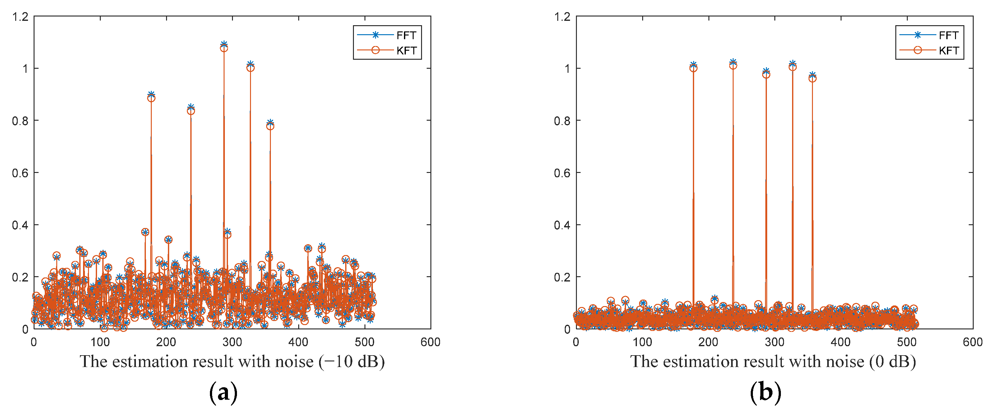
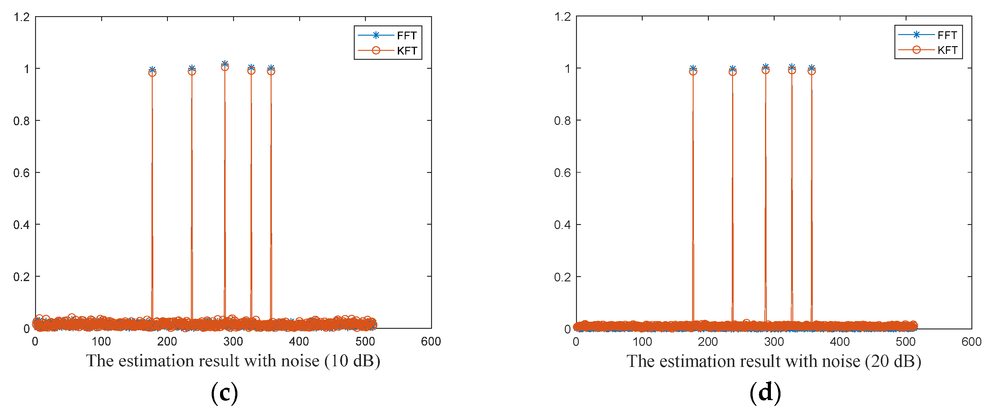
The DFT is applied here to obtain the frequency components of the signal, which can be used as the reference to the estimated result of the KF-tracking algorithm. The simulation results under different SNR levels
are presented in
Figure 2, where the blue line with star (‘*’) and red line with circle (‘o’) denote the results of the DFT and KF-tracking methods, respectively.
From the
Figure 2, we can see that the KF-tracking method can recover the signal in frequency domain the same as the Fourier transform method based on the data and in the KF-tracking algorithm,
, where
denotes the total KF-tracking number. This case is the full aperture case to verify that the KF-tracking algorithm works.
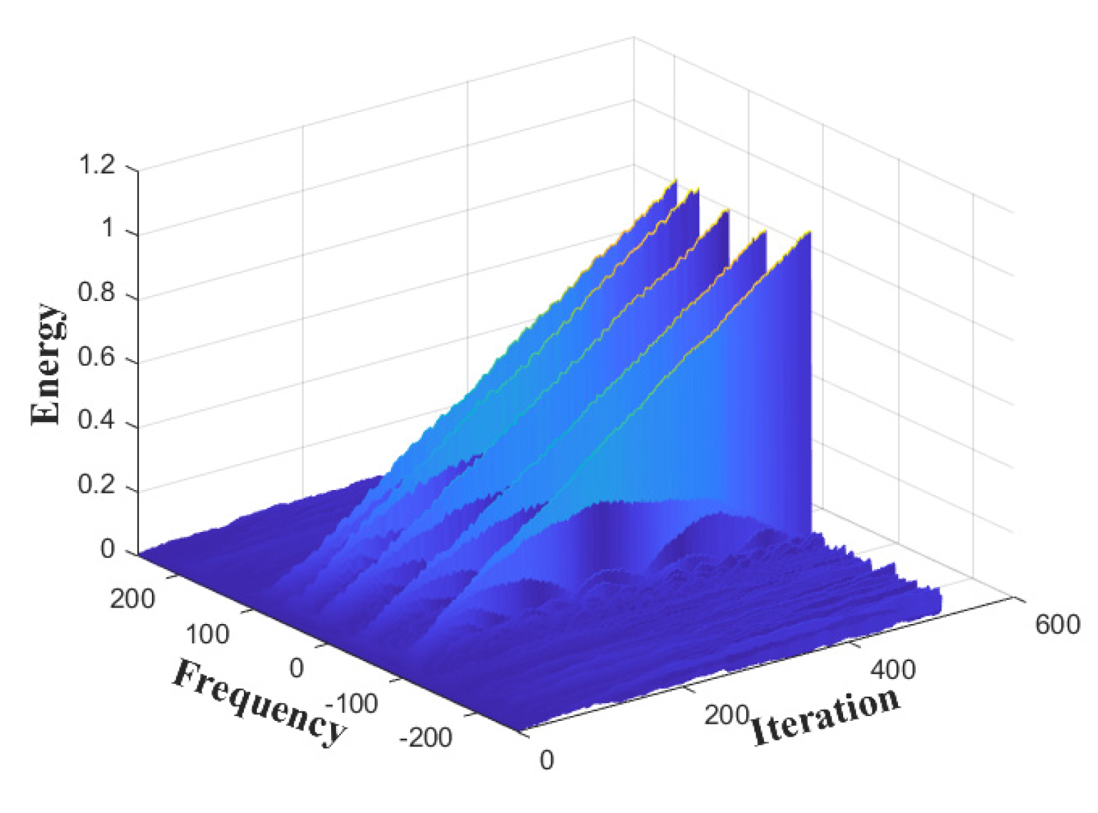
Based on the principle of the KF-tracking method (as analyzed in
Section 3), the frequency separation of
is estimated and corrected at each iteration, which can make the state vector gradually getting focused. The corrected state vector at each iteration is demonstrated in
Figure 3, where SNR is
.
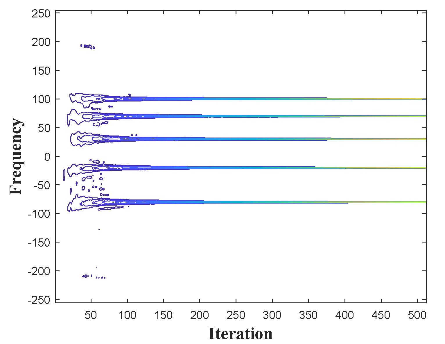
Figure 3 shows the accumulation process of the state vector at each iteration. At the beginning, the state vector is initialized as a zeros vector, as iteration continues, the energy of the signal is accumulated towards the true value of the state vector. In order to better demonstrate the accumulation process, we extract the main components of the recovered signal, which are shown in
Figure 4.
From
Figure 4, we can see that the main components are gradually focused at the positions
in the Doppler domain as we formulated at the beginning. In addition, it is obvious to see that after 100 iterations, the recovered state vector is close to the true value. The KF-tracking method can accomplish the recovering procedure in a short iteration, which denotes the short observation aperture. This means that when
, the KF-tracking algorithm works well already.
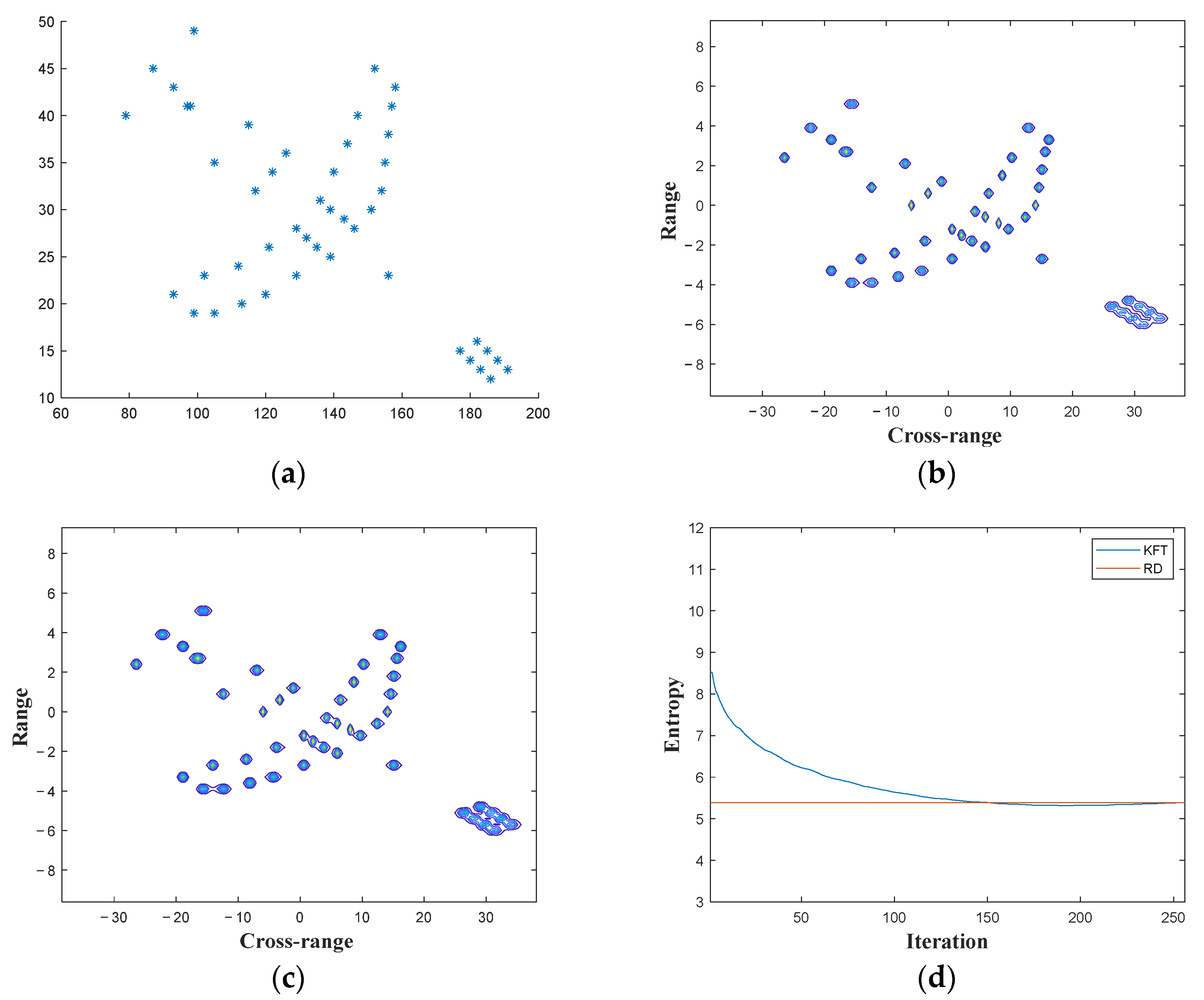
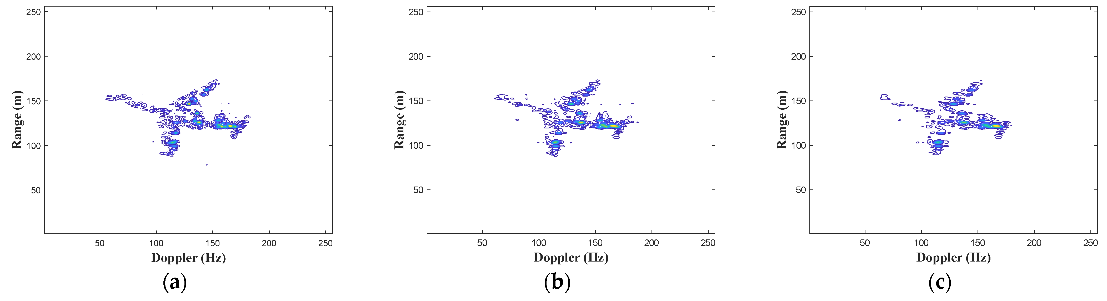
A group of simulated radar echoes of a uniformly rotating target are applied here to demonstrate the performance of the proposed KT-tracking method on recovering an ISAR image. The total number of the full apertures is
. The 2D scatter model of the plane target is presented in
Figure 5a and the rotating vector is perpendicular to the 2D plane. The simulation results of full aperture returned signals are presented in
Figure 5b,c, where
Figure 5b is the image of the plane target using the RD algorithm and
Figure 5c shows the result applying the proposed frequency KF-tracking method with
.
The blue curve in
Figure 5d shows the entropy of the recovered signal at each iteration while the red line denotes to the entropy of the RD imaging algorithm. The entropy of the recovered image using KF-tracking is gradually close to the red line and almost at 110th iteration reached the same entropy, which means the KF-tracking method can obtain the same imaging quality with less observing data.
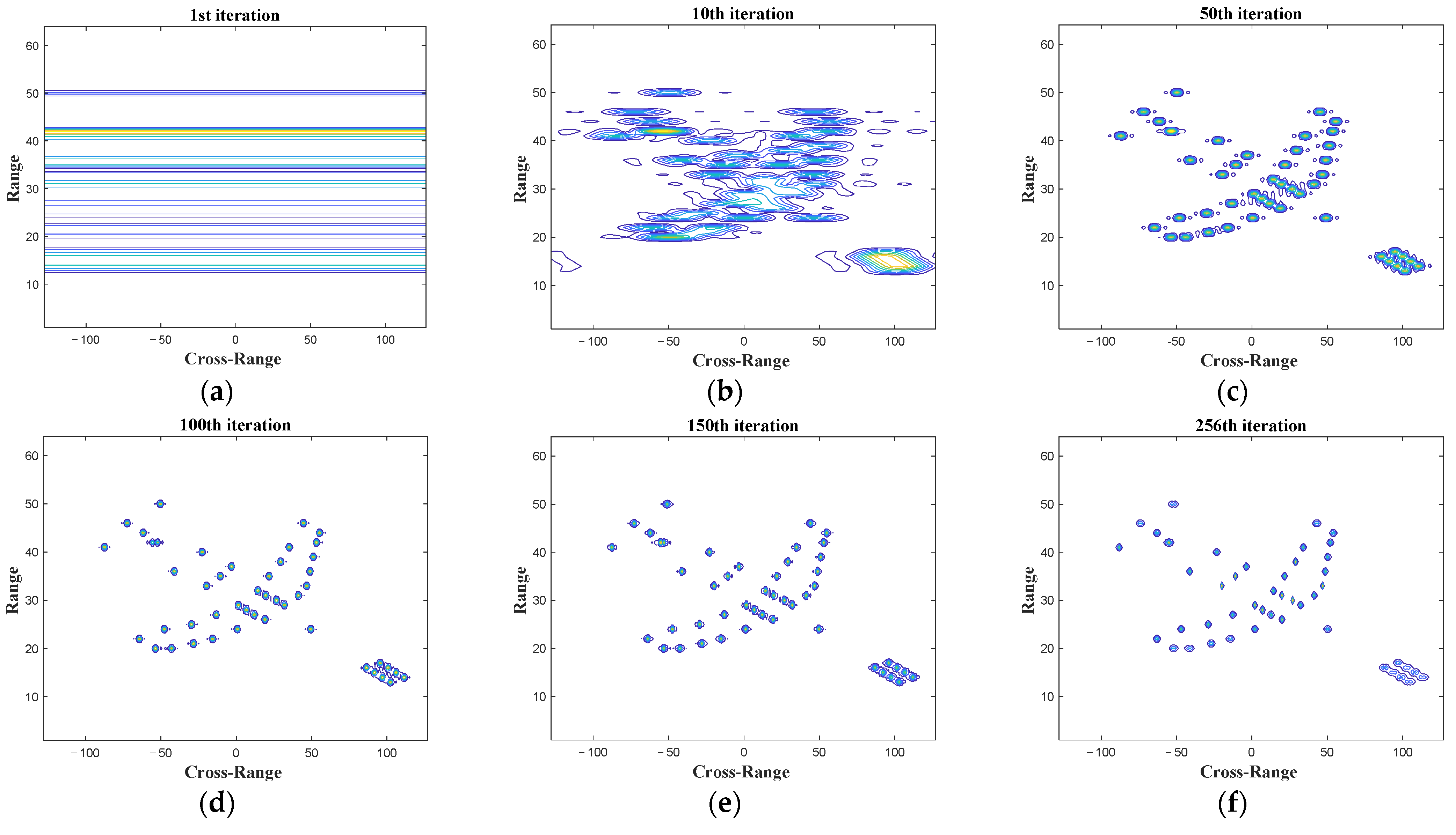
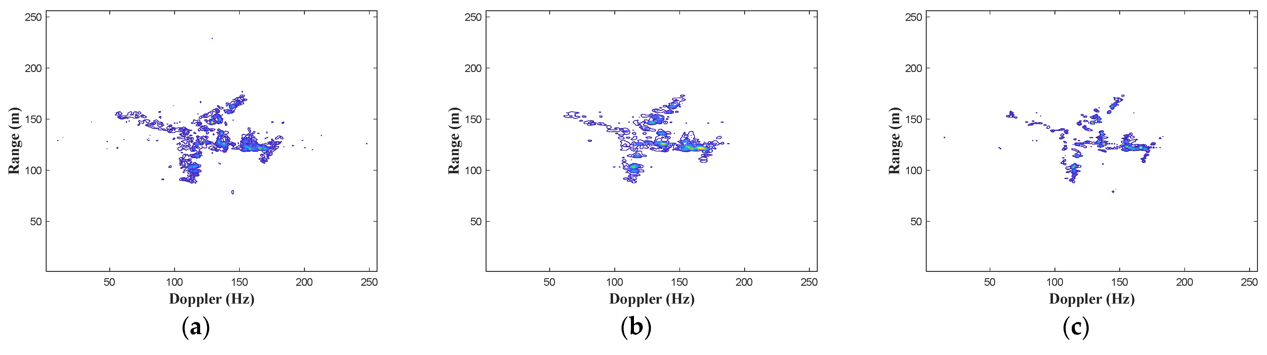
In addition, according to the principle of KF-tracking method, we can obtain the recovered image at each iteration. So, we select a series of recovered images of selected iterations
and present these images in
Figure 6.
From
Figure 6, we can see that, at the 10th iteration, the cross-range resolution of the recovered image is low. As KF-tracking continues, the recovered image gets focused close to the accurate image. At the 50th iteration, we can see that the imaging quality is improved. Compared
Figure 6d with
Figure 5b, the image obtained by KF tracking method at 100th iteration, i.e.,
, has the same quality as the image obtained by the RD method with full aperture data, i.e.,
. The KF-tracking mainly relies on the relationship of the state changing and the observation value of the current state.
Figure 6 illustrates that in a short observation iteration, the high cross-range resolution image can be obtained by KF-tracking method.
Then, we select half of the full aperture, i.e.,
and
of the simulated plane data and add noise to the data with
different SNR levels (20
,10
,5
). To better demonstrate the anti-noise ability of the KF-tracking method when recovering a high-resolution image,
, from a short aperture,
, data, the burg interpolation method [
14] and Relax method [
17] are applied here as compared methods. The range profiles of the data at the three different noise levels are shown in
Figure 7. The simulation results are presented in
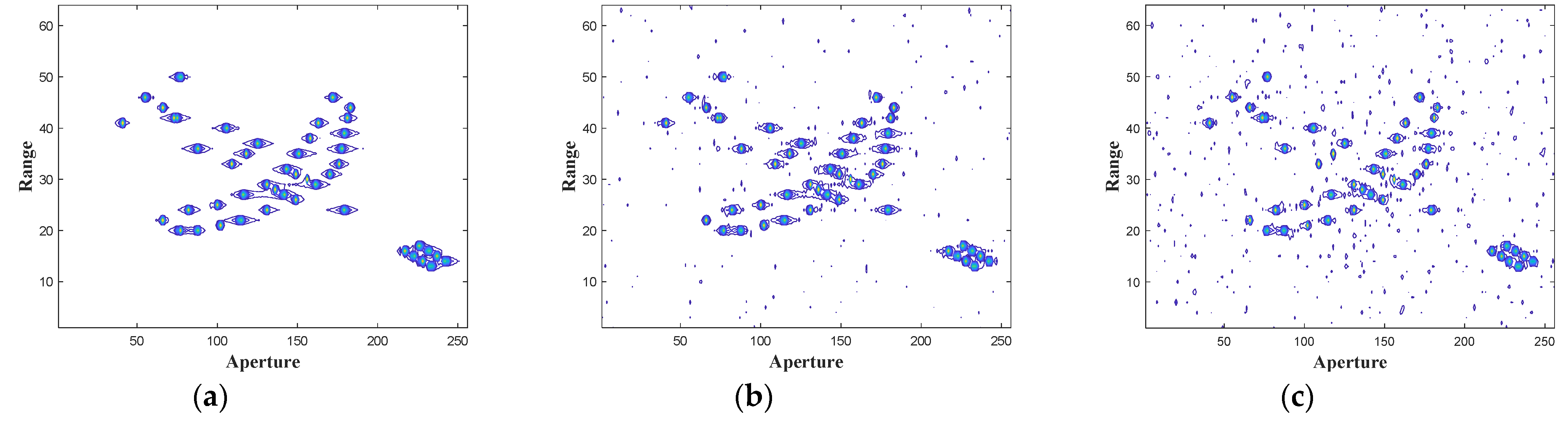
Figure 8,
Figure 9 and
Figure 10, respectively.
From the three images of each figure, we can see, the higher the noise level is, the lower imaging quality is. Comparing the images with the same noise level between each figure, we can see, the burg and Relax methods generate lots of noise pixels under the low SNR. Thus, we can see that under low SNR conditions, the anti-noise ability of KF-tracking method is better than the other two methods.
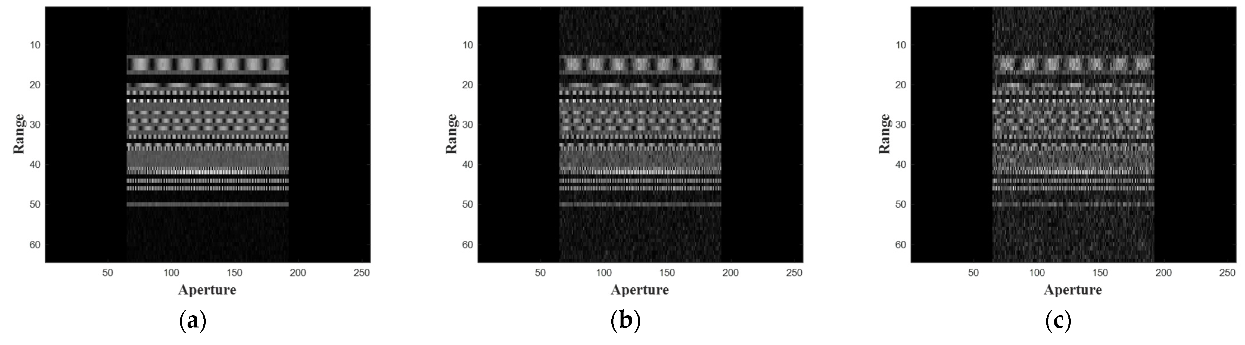
5. Real Data Results
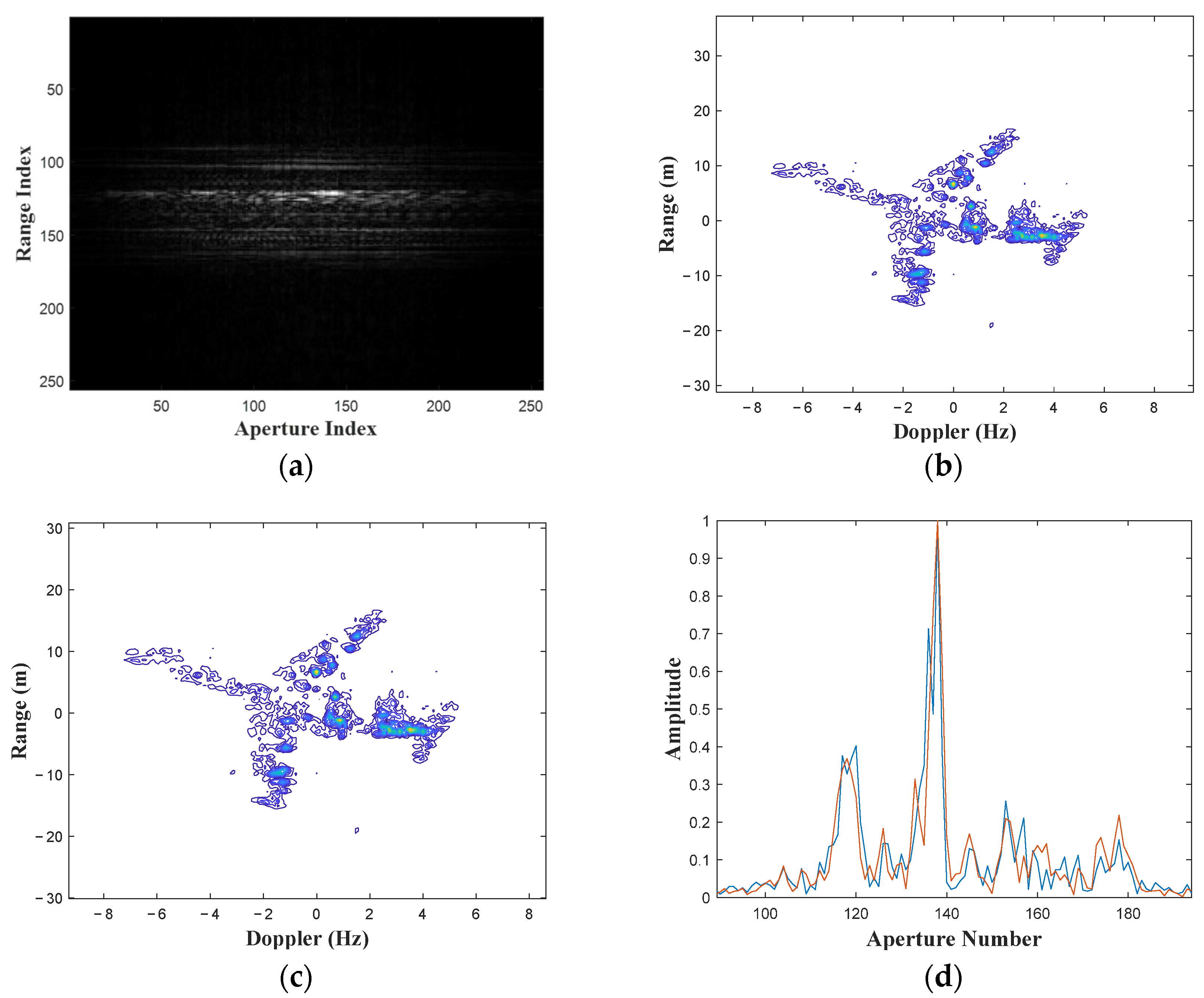
The proposed KF-tracking method is further tested on the real data of the Yake-42. The real data is a C-band collection with 400-MHz bandwidth. The PRF is 25 Hz while the observation interval is 10.24 s. The total number of the apertures is .
Figure 11a is the returned signal after the range compression and motion compensation.
Figure 11b denotes the ISAR image of the full aperture data applying the RD method. The recovered image using the proposed method is presented in
Figure 11c.
From
Figure 11c, we select an isolated scatter, at the position (138,126) circled with the red circle and extract the 126th range profile including this scatter.
Figure 11d shows the 126th range profiles of the recovered signals, where the blue line is from the RD method and the red line denotes the result of the KF-tracking method.
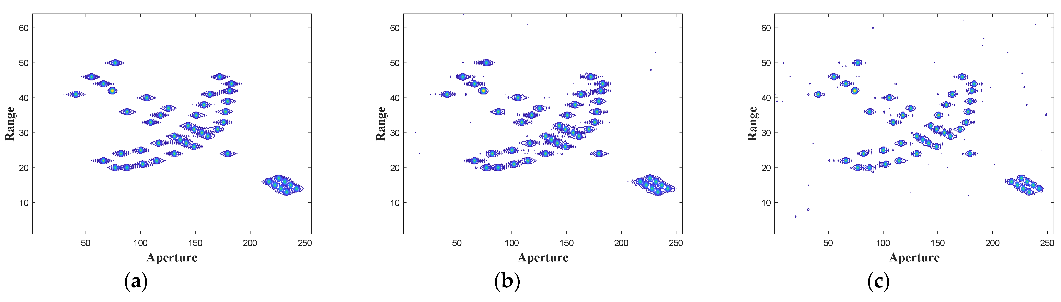
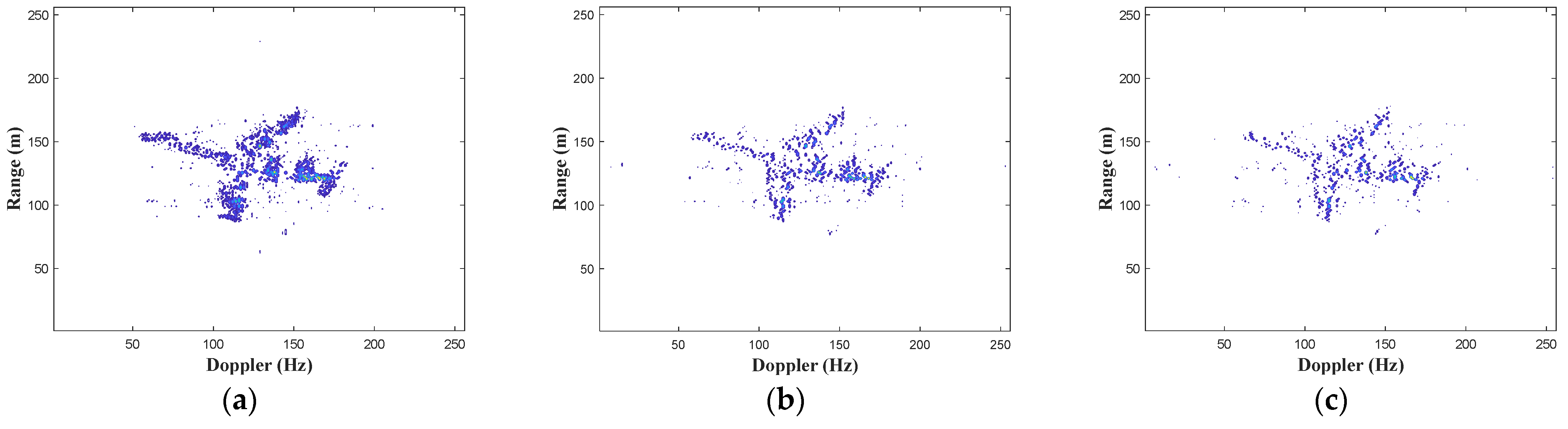
Then, we extract
= 128, 64 and 32 pulses to demonstrate the performance of the KF-tracking method, respectively. The high-resolution imaging results
of the KF-tracking method, burg and relax methods are presented in
Figure 12,
Figure 13 and
Figure 14, respectively.
Compared to the recovered images of the three methods, we can see that the KF-tracking method can obtain the high-resolution image of the target in a short observation aperture. However, when the number of the received pulses decreases, some details of the images are getting lost. The KF-tracking can still recover the image of the target and has the least noise pixels.


