Abstract
For Global Positioning System (GPS) precise orbit determination (POD), the solar radiation pressure (SRP) is the dominant nongravitational perturbation force. Among the current SRP models, the ECOM and box-wing models are widely used in the International GNSS Service (IGS) community. However, the performance of different models varies over different GPS satellites. In this study, we investigate the performances of different SRP models, including the box-wing and adjustable box-wing as a priori models, and ECOM1 and ECOM2 as parameterization models, in the GPS POD solution from 2017 to 2019. Moreover, we pay special attention to the handling of the shadow factor in the SRP modeling for eclipsing satellites, which is critical to achieve high-precision POD solutions but has not yet been fully investigated. We demonstrate that, as an a priori SRP model, the adjustable box-wing has better performance than the box-wing model by up to 5 mm in the orbit day boundary discontinuity (DBD) statistics, with the largest improvement observed on the BLOCK IIR satellites using the ECOM1 as a parameterization SRP model. The box-wing model shows an insignificant orbit improvement serving as the a priori SRP model. For the eclipsing satellites, the three-dimensional (3D) root mean square (RMS) values of orbit DBD are improved when the shadow factor is applied only in the D direction (pointing toward to Sun) than that in the three directions (D, Y, and B) in the satellite frame. Different SRP models have comparable performance in terms of the Earth rotation parameter (ERP) agreement with the IERS EOP 14C04 product, whereas the magnitude of the length of day (LoD) annual signal is reduced when the shadow factor is applied in the D direction than in the three directions. This study clarifies how the shadow factor should be applied in the GPS POD solution and demonstrates that the a priori adjustable box-wing model combined with ECOM1 is more suitable for high-precision GPS POD solutions, which is useful for the further GNSS data analysis.
1. Introduction
The Global Positioning System (GPS) serves as a critical role in the positioning, navigation, and timing (PNT) services and is also a powerful tool in monitoring and understanding the geophysical processes of the Earth system [1,2], crust movement [3,4], and meteorological studies [5,6]. The International GNSS Service (IGS) community has been making continuous efforts in understanding the errors and further improving satellite orbit dynamic modeling. Currently, the GPS orbit products from IGS and other analysis lefts (ACs) have a one-dimensional (1D) mean error of around 1 cm in terms of inter-AC agreement [7] and 2.5 cm root mean square (RMS) in terms of the satellite laser ranging (SLR) validation [http://www.igs.org (accessed on 9 January 2021)]. One of the major nongravitational forces affecting the current GPS orbits is the solar radiation pressure (SRP), which relies on the knowledge of satellite-related properties. Although many SRP models have been developed, the performance of different SRP models have not been fully investigated, especially considering the different type of GPS satellites and the performances in eclipse seasons [8]. Note that the eclipse season in this study means that the β angle, that is, the elevation angle of the Sun over orbital plane, is within ±13.25° [9].
The SRP models are mainly divided into two categories, the analytical and empirical models. Analytical models such as the box-wing and ray tracing approach are established based on the physical properties of the satellite components, including the area, reflection, diffusion, absorption, and the satellite attitude. The attitude control modes of GPS satellites are known clearly except for BLOCK IIA satellites during eclipse seasons. The satellite shapes, area, and optical properties were published for the BLOCK I, II, IIA, IIR [10,11], and IIF satellites [12]. Despite the analytical models having a clear physical interpretation, they can still cause large model errors due to the possible inaccurate satellite structure or optical property. There are two feasible methods to avoid the deviations of these model from the reality. The first one is to adjust optical coefficients with satellite tracking data [13]; for instance, the adjustable boxing-wing modeling considering potential additional acceleration was established using ten years of GPS observations for the GPS BLOCK IIA, IIR, and IIF satellites [8]. The second one is to develop an expression of Fourier series based on the analysis of accelerations caused by SRP, such as the ROCK model series (ROCK-S, ROCK-T), which was first developed by the satellite manufacturer Rockwell International [10,11,14,15], and the GSPM (GPS solar radiation model) developed by JPL (Jet Propulsion Laboratory) [16].
In addition to the models derived from physical-based methods, the empirical SRP models are developed by fitting the long-term orbit estimates regardless of the satellite metadata—for instance, the Empirical CODE Orbit Model (ECOM) developed by left for Orbit Determination in Europe (CODE) [17]. The ECOM was then further refined by reducing the periodic terms in the satellite–Sun direction, that is, the ECOM1 model with five coefficients [18]. The ECOM2 was developed in 2015 to consider the SRP variation caused by different satellite shapes—for instance, the Galileo satellites [19]. Both ECOM1 and ECOM2 are widely used as parameterization models by several ACs [20,21,22]. However, estimating more parameters in ECOM2 can cause an overparameterization and destabilize orbit solutions, and the pure parameterization models may also introduce draconitic errors in GNSS-based geodetic products [23,24]. To minimize the number of SRP parameters and consider the SRP force components that cannot be described by the parameterization model, an a priori SRP model is recommended [25]. Hence, a hybrid strategy of combining the a priori box-wing model and the parameterization model, that is, ECOM1 or ECOM2, has been proved to be beneficial for the orbit quality [8,26,27,28].
The GPS satellite orbit differences between different ACs have been proved to be largely caused by different approaches of SRP modeling [29]. It was also reported that the performances of different SRP modeling in GPS POD are related to specific satellite types, as most of the BLOCK IIR satellites have different performances [30]. For instance, ECOM1 has better performance than ECOM2 in terms of predicated orbit precision [31]. In addition, an analysis for Chinese BeiDou satellite navigation system (BDS) IGSO and MEO orbits indicated that the box-wing model can remove the β- and μ-dependent systematic orbit errors [32]. All the analyses mentioned above have summarized the diversity of GPS orbit precision between using ECOM1 and ECOM2 and the importance of the a priori box-wing model. Despite the above studies, a comprehensive investigation of different SRP models especially when GPS satellites are in eclipse seasons is still lacking.
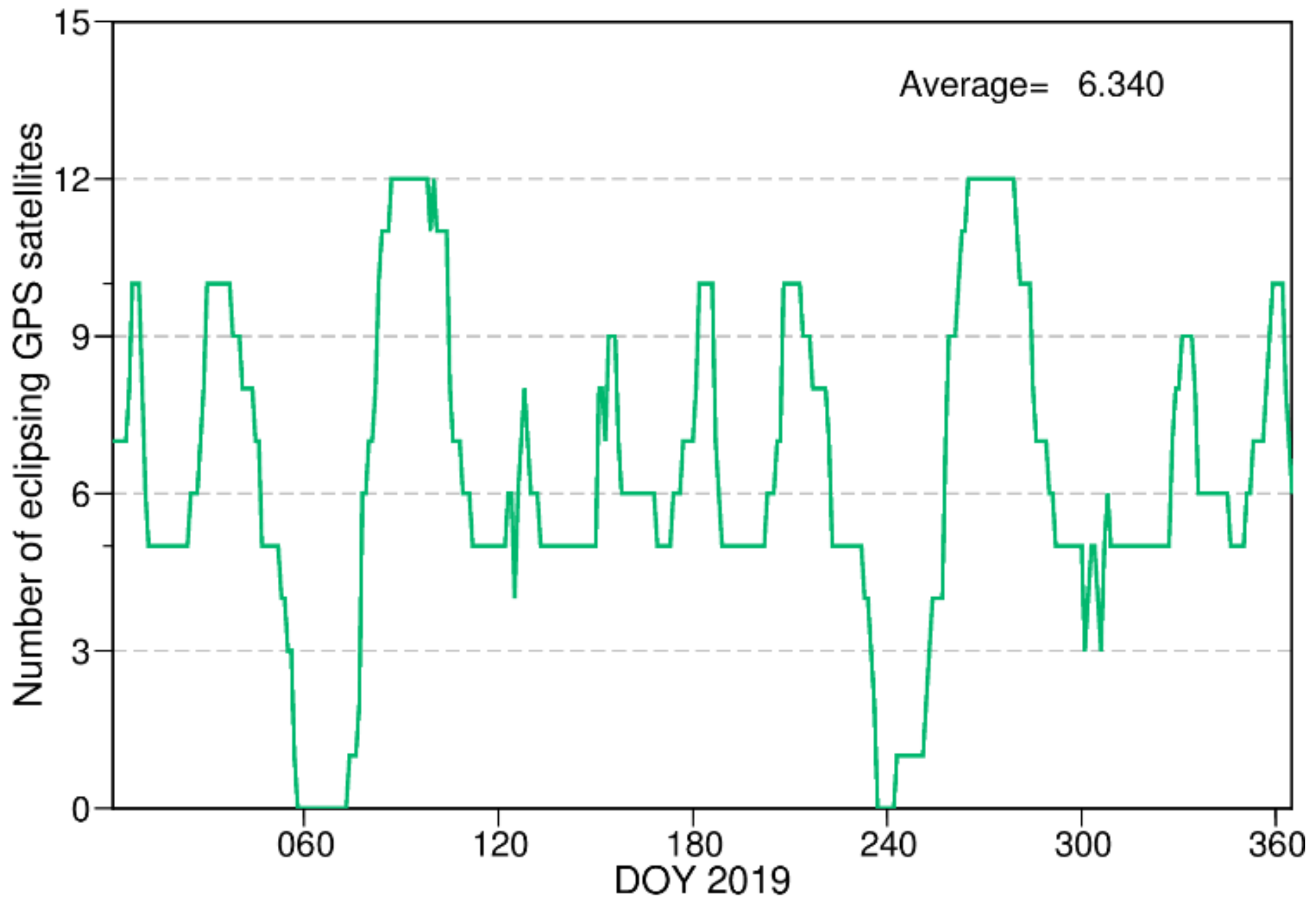
When a satellite enters the umbra or the penumbra area of the occulting bodies (usually the Earth and the Moon), that is, the eclipse season, a shadow factor is adopted to represent the degrees of Sun occultation. Different ACs adopt different strategies, either in all D direction, which is the satellite–Sun direction, Y direction, which is the solar panel axis direction, or B direction, which completes the right-hand orthogonal system adopted by GeoForschungsZentrum (GFZ) (Zhiguo Deng, personal communication, 10 February 2020), or only in the D direction adopted by Wuhan University (WHU) (Jin Guo, personal communication, 22 February 2020). Although several studies tried to refine its function model, few studies focus on the relationship between shadow factor and the parameterization model and its impact on eclipsing satellites. The eclipse seasons are quite common for GPS satellites. Figure 1 shows that among the 32 operational GPS satellites in 2019, the average number of eclipsing satellites is around 6 and the maximum number is 12, and a single eclipse event lasts 40 min on average. Moreover, some unmodeled non-SRP forces may exist and will become conspicuous for those satellites during eclipsing season, which cannot be neglected [8,33]. Therefore, it is necessary to investigate the orbit accuracy during eclipse seasons and clarify the proper method of combining shadow factor and the parameterization SRP model.
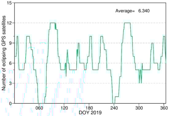
Figure 1.
Daily number of GPS satellites in eclipse seasons in 2019.
Therefore, the major motivation of this study is to evaluate different combinations of the a priori box-wing model and the parameterization model (that is, ECOM1 or ECOM2), and the application of the shadow factor, focusing on eclipsing satellites. Following this introduction, the SRP models and the shadow function are described in Section 2. After a short description of data processing strategies in Section 3, the results are analyzed in Section 4, where the orbit quality is evaluated by the day boundary discontinuity (DBD), and Earth rotation parameters (ERPs) are evaluated by comparing to the IERS EOP 14C04 product. The main findings are summarized and the future perspectives are given in Section 5.
2. Methodology
The acceleration of an in-orbit satellite caused by SRP perturbation can be expressed as:
where denotes acceleration derived from an a priori model and denotes the acceleration represented by a parameterization model to be estimated. In the third IGS reprocessing campaign, the ECOM2, JPL GSPM, or box-wing model combined with ECOM1 is suggested for the GPS satellites except for the BLOCK IIR and IIF, for which the ECOM1 is recommended (http://acc.igs.org/repro3/repro3.html (accessed on 9 May 2021)). For the SRP modeling analysis in this study, we use the box-wing model as the a priori model and ECOM1 or ECOM2 as the parameterization model.
The a priori acceleration can be expressed as [13]:
where denotes the squared ratio between satellite–Sun distance and Earth–Sun distance; denotes the area of surface; denotes the mass of the satellite; denotes the solar flux at ; denotes the velocity of light in vacuum; , , and denote the fractions of absorbed, specularly reflected, and diffusely scattered photons, respectively; denotes the thermal radiation factor (1 for satellite body and 0 for solar panel); denotes the unit vector from satellite to Sun; denotes the unit normal vector of surface; and denotes the angle between and . For the adjustable box-wing model, the optical parameters are updated by tracking data.
The acceleration of the parameterization SRP model can be expressed as:
where denotes the satellite’s argument of latitude, denotes the unit vector in the D direction, denotes the unit vector in the Y direction, and denotes the unit vector in the B direction. In ECOM1, the functions , , and are represented as a truncated Fourier series [18],
where , , and are constant terms and and are first-per-revolution terms. Compared to the ECOM1 model, the twice-per-revolution and fourth-per-revolution terms are added in the D direction in the ECOM2 modeling, while is replaced by the angular argument and is the Sun’s argument of latitude in satellite orbital plane for straightforward interpretation [19].
Considering the IGS conventional body-fixed frame [34], its relationship with the DYB frame can be presented as:
where
and denotes the elevation angle of the Sun over the orbital plane.
When a satellite enters the eclipse season, a shadow factor is usually employed to describe the corresponding solar irradiance variation. Adopting the conical shadow model, the shadow factor can be calculated in the following three cases:
- Full phase: the Sun is fully visible to the satellite, therefore ;
- Penumbra: the satellite is in the penumbra area of the Earth and the Moon and it can receive only part of the solar irradiance from the Sun, therefore [35] (pp. 81–83):where denotes the total area of the Sun occulted by the Earth and the Moon, and the apparent radius of the Sun;
- Umbra: the satellite is in the umbra of satellite, therefore
If the shadow factor is applied in Equation (1) in three directions, which is used by CODE and GFZ, Equation (1) can be rewritten as:
If the shadow factor is applied in Equation (1) only in the D direction, which is used by WHU, Equation (1) can be rewritten as:
The term usually consists of two parts. The first part is the instrument bias, namely the yaw bias, which is caused by the misalignment of solar panels or solar sensor errors and observed for BLOCK II and IIA satellites [10]. The second one is the thermal radiation, which was found on the Y surfaces (radiated from louvers) of the BLOCK IIR satellites [36]. The thermal radiator is designed for evacuating excessive heat from onboard payloads to space, and as a result, an additional force is generated. However, thermal control information of the GPS satellites is not available to the public, which is hardly to model and cannot be easily included as an a priori SRP model. Ignoring these small forces, for example, using Equation (8) can degrade the orbit accuracy in the eclipse season. An inspection of Equation (9) shows that keeping the active during the Earth’s shadow transitions can help to model the thermal radiation during eclipse seasons, along with other possible non-SRP nature forces in Y surfaces. In addition to the surfaces, the and surfaces may also undergo thermal radiations. Assuming there is a constant acceleration in the surface and it can be represented as , 0, and in the D, Y, and B directions, respectively. Similarly, assuming there is a constant acceleration in the surface and it can be represented as , 0, and in the D, Y, and B directions, respectively. Therefore, these constant accelerations corresponding to the B direction can be modeled by the 1 cycle per revolution (cpr) terms in both ECOM1 and ECOM2 because of their 1 cpr terms, whereas the rest part corresponding to the D direction can only be partially modeled in ECOM1 and ECOM2, where ECOM2 has better performance due to its additional 2 and 4 cpr terms.
In addition to the above-mentioned potential thermal radiations, there are other potential nonconservative forces that need to be considered during eclipse seasons—for example, a surface undergoing heating up and cooling down periods during shadow transitions, active thermal control of shadow season, etc. If there are thermal radiation or other unmodeled nonconservative forces in Y or other surface, keeping parameters in the Y and B directions active in the eclipse season can compensate for the forces of non-SRP nature to some extent, and we will continue to prove this inference in Section 4.
3. Data Processing Strategy
In Section 2, we presented the SRP modeling, the ways of applying the shadow factor, and its relationship with possible unmodeled or inaccurately modeled non-SRP forces. As the ECOM2 has more periodic terms than ECOM1 in the D direction, it may have different behaviors for eclipsing satellites. In this Section, we introduce our analysis methods on evaluating the performance of different SRP models, with an emphasis on satellites in eclipsing seasons.
Combining the strategies of using ECOM1 or ECOM2 as the parameterization model, using no model, the box-wing, and adjustable box-wing model as a priori model, and the application of the shadow factor, i.e., in the D or DYB directions, we have 12 different solutions, as shown in Table 1. For the box-wing model, we use satellite metadata and optical properties provided by the manufacturers [10,11], and for the adjustable box-wing model, we use adjusted metadata and optical properties provided by Duan [8]. From the results listed in Section 4, we infer that each satellite may suffer different magnitudes of unmodeled forces, even for the same block type. The established box-wing model does not contain this term. Considering that the purpose of this work is to evaluate different SRP models and shadow factor, we do not introduce the additional accelerations in either X or Y surfaces provided by Duan et al. [8], which are applied for remaining forces after employing the adjustable box-wing model.

Table 1.
Twelve cases of GPS daily precise orbit determination solutions using different methods in handling the a priori model, the parameterization model, and the shadow factor. Note that the directions in which shadow factor is applied refers to the parameterization model, and in the a priori model, the shadow factor is always applied. See Equations (8) and (9) for details.
The GPS observations from the year of 2017 to 2019 were processed on a daily basis, using the Positioning And Navigation Data Analyst (PANDA) software [37]. More details are given in Table 2.
Table 2.
Data processing strategy of GPS precise orbit determination solution.
To minimize the possible errors caused by integration, the Adams–Bashforth–Moulton predictor–corrector integration method is switched to the Runge–Kutta–Fehlberg (RKF) integration method during the shadow transition, that is, the period from full phase to umbra or inverse.
Unlike the GLONASS, Galileo, and BeiDou satellites where the SLR tracking observations are available, the GPS BLOCK IIA, IIR, IIF, and III satellites used in this study are not equipped with retroreflector arrays, and thus using SLR as an external orbit validation is not possible [47]. It is also not optimal to use the orbit products form the IGS ACs as a reference for comparison, as their SRP modeling and strategies of applying the shadow factor are different with each other and can affect the orbit product. Therefore, the following quantities are used to assess the different solutions:
- Analyses of the estimated SRP parameters: the estimated ECOM parameters should not show systematic biases if the a priori model can describe all important characteristics of the satellite. The correlation between the satellite orbit dynamic parameters can also measure the association of these parameters;
- Day boundary discontinuities (DBD) of the satellite orbits: 3D distance between the orbital positions of two consecutive arcs are commonly used to assess the internal consistency of the orbit solution;
- Agreement of the Earth rotation parameters (ERPs) to the IERS EOP 14C04 product [45]: the GPS technique provides precise polar motion and LoD estimates, and thus the ERP estimates from different solutions can be compared to the IERS product. We calculated the weighted STD (WSTD) of the differences between the GPS POD solution and the IERS 14C04 product [48] as:
4. Results and Discussions
In this Section, we first analyze the orbital parameters in Section 4.1 and the orbit precision of the BLOCK IIR and IIF satellites in Section 4.2, and then present the ERP agreement with the IERS EOP 14C04 product in Section 4.3. For the orbit precision analyses, the BLOCK IIA satellites are not presented because precisely modeling its postshadow recovery can be difficult [49] and only one or two satellites are in operation during the time span. The newly employment BLOCK III satellites are also not included, as the adjustable box-wing model is not available until now and they may undergo outgassing phase at their initial operation period, which will influence the comparison [14].
4.1. Estimated ECOM Parameters
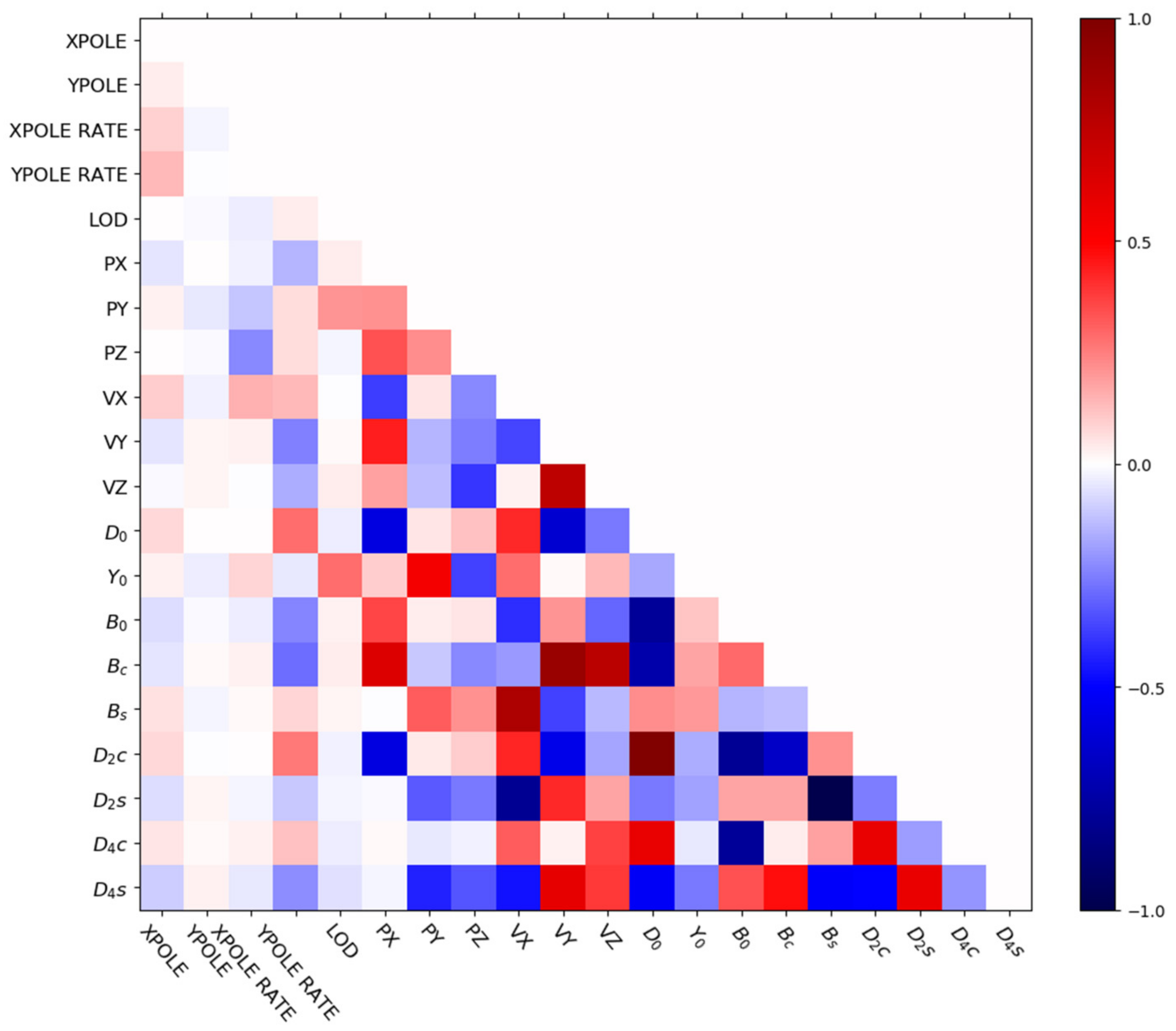
To investigate the correlation between ECOM SRP parameters, Figure 2 and Figure 3 show the correlation coefficients in the E2DYB solution among the estimated satellite dynamic parameters of G067, a BLOCK IIF satellite, and EPRs () during noneclipsing and eclipsing seasons, respectively. We can see that in both higher and lower angles, the term is highly correlated with the and terms, with correlation coefficients larger than 0.9 and 0.6, respectively, and the correlation between and term is close to −1, which means that they are highly correlated. Similar correlation can also be observed for the BLOCK IIR satellites (not shown here). Comparing Figure 2 and Figure 3, we can see that the correlation coefficients are higher in eclipse seasons, i.e., the coefficients between and , and and at lower β angle are larger than that at the higher . Consequently, the SRP parameters in the D direction can be hardly separated from the parameters in the Y and B directions, as is the interaction between the different ECOM parameters when satellites are at lower angle.
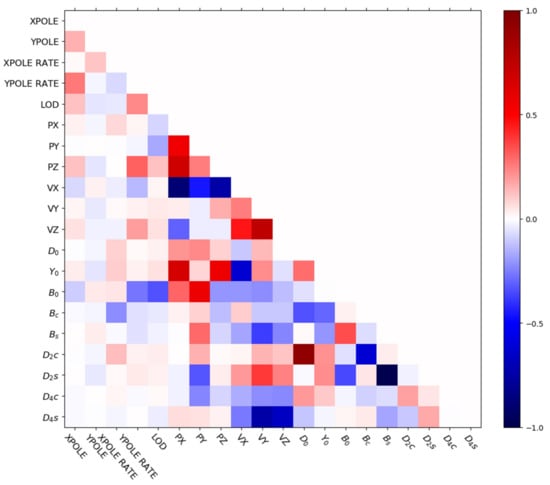
Figure 2.
Correlation coefficients between the Earth rotation parameters and the satellite dynamic parameters using the ECOM2 as a parameterization model (E2DYB solution) for G067 (BLOCK IIF) in noneclipsing season ().

Figure 3.
Correlation coefficients between the Earth rotation parameters and the satellite dynamic parameters using the ECOM2 as a parameterization model (E2DYB solution) for G067 (BLOCK IIF) in eclipsing season ().
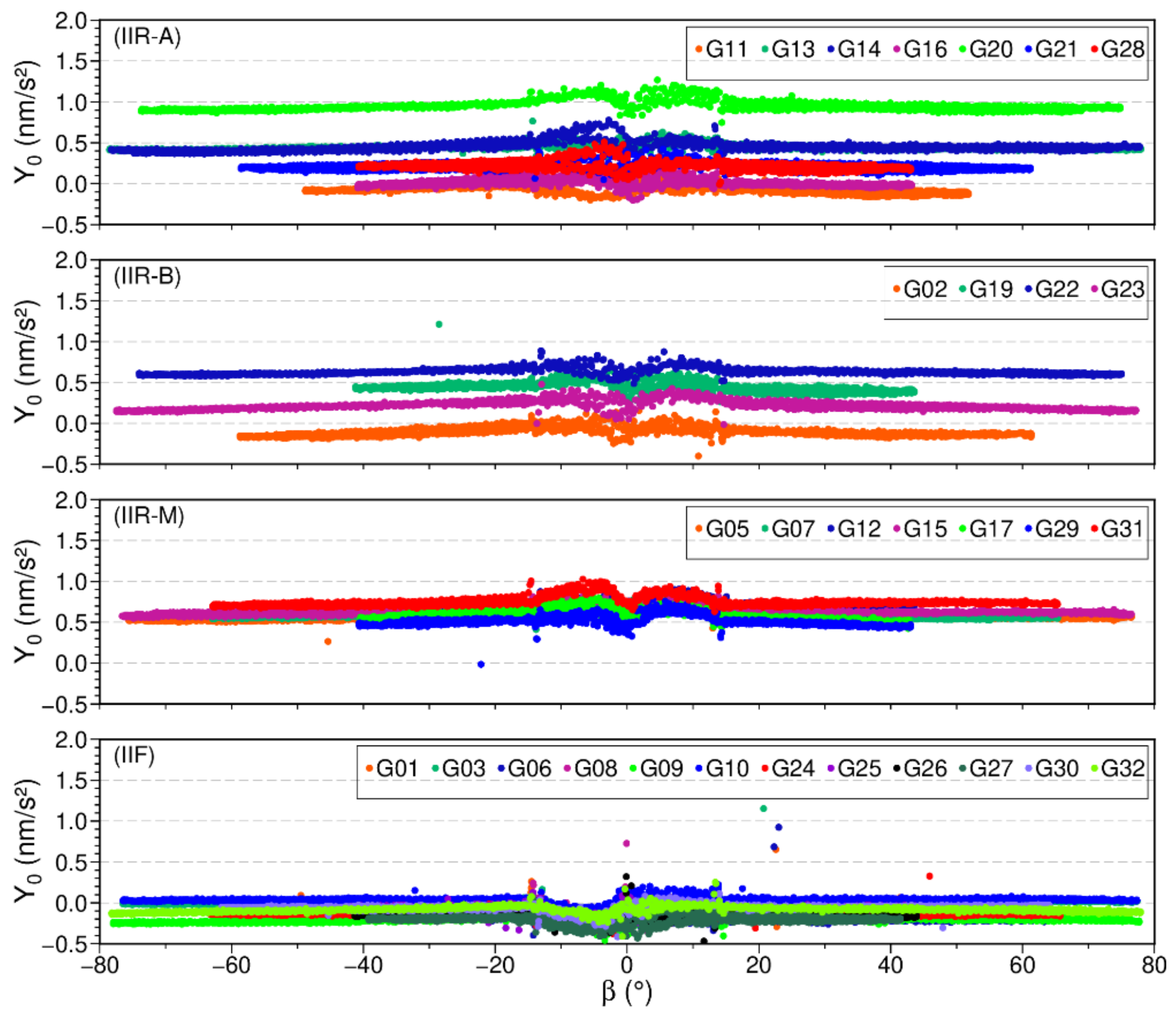
Figure 4 presents the time series of estimated for all BLOCK IIR and BLOCK IIF satellites in the E1DYB solution. The BLOCK IIR satellites show a larger value than the BLOCK IIF satellites, which exhibits as a constant acceleration along the satellite Y-axis, that is, the Y-bias. As the accelerations caused by yaw bias are related to the Sun irradiation, the term can be omitted as Equation (8) represented if it is dominated by the yaw bias. The magnitude of perturbations caused by the yaw bias for BLOCK IIR satellites is about 0.15 [8], which is consistent with the behavior of Galileo Full Operational Capability (FOC) satellites [33,50]. However, most of the estimated coefficients for BLOCK IIR satellites are larger than 0.5 , indicating that there are possible thermal forces in the Y direction. Taking unmodeled non-SRP forces, Equation (9) is more reasonable than Equation (8). It is noteworthy that the highest dispersion is visible for the legacy BLOCK IIR-A and BLOCK IIR-B satellites (the upper two panels in Figure 4), and the largest difference is greater than 0.4 , whereas the variation of the coefficient is less significant for Block IIR-M and BLOCK IIF satellites (the lower two panels in Figure 4). This diversity means the magnitude of thermal forces are different between the BLOCK IIR-A, BLOCK IIR-B, and BLOCK IIR-M satellites.

Figure 4.
SRP coefficient with respect to the β angle (the Sun elevation above the orbital plane) in the E1DYB solution from 2017 to 2019. From top to bottom: BLOCK IIR-A, BLOCK IIR-B, BLOCK IIR-M, and BLOCK IIF satellites, respectively.
For a further comparison of Equations (8) and (9), taking SVN G050 (BLOCK IIR) and G073 (BLOCK IIF) as an example, the estimated coefficients in the Y and B directions derived from the E1D and E1DYB solutions are shown in Figure 5. The coefficients of SVN G050 in the B direction are shifted by 6 for better view. As we can see, the estimated coefficient derived in the E1D solution shows less scatter between the phases in and out of eclipse seasons. A similar pattern was also reported when an a priori box-wing model was used (see Figure 15 in [50]). It indicates that BLOCK IIR satellites have a relatively noticeable thermal radiation in Y surfaces. In addition, the estimates of BLOCK IIF satellite (SVN G073 in Figure 5) have a visible linear trend during eclipse seasons and are reduced after the angle switches the sign (see Figure 4 in [8]). This needs further investigation. In contrast to the of BLOCK IIR satellites, the trend of (for instance, SVN G073) shows larger variation.
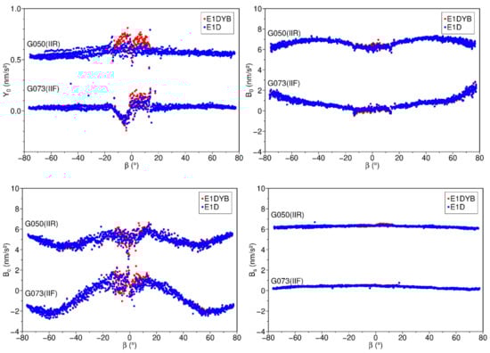
Figure 5.
SRP coefficients (upper left), (upper right), (lower left), and (lower right) with respect to the β angle in solution E1DYB (red dots) and solution E1D (blue dots) spanning from 2017 to 2019. The results of SVN G050 are all shifted by 6 for better visualization, except for the coefficient . Note the different y-axis scales between the upper-left panel (the panel) and the others.
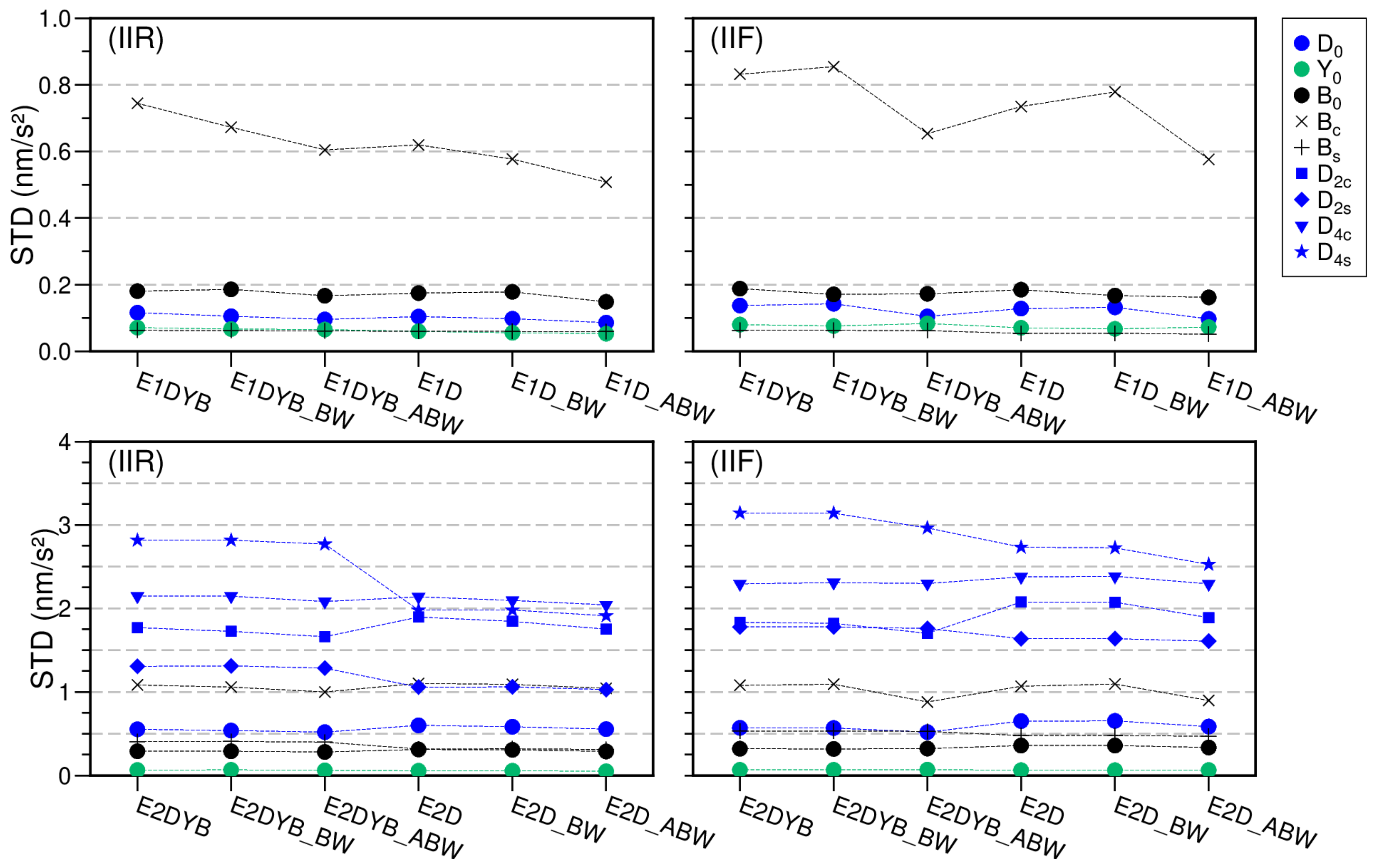
Furthermore, the standard deviation (STD) values of SRP parameters in the 12 solutions are given in Figure 6. For the ECOM1 solutions (that is, using ECOM1 as the parameterization model) shown in the upper panels of Figure 6, the STD of the (marked with black X-cross) is improved when an a priori box-wing model is used or a shadow factor is applied only in the D direction, except for BLOCK IIF satellites, whereas other coefficients have comparable STD values between different solutions. The STD difference of between solution E1DYB and solution E1D_ABW is around 0.2 for BLOCK IIR satellites and BLOCK IIF satellites. As for the ECOM2 solutions (that is, using ECOM2 as parameterization model) shown in the lower panels in Figure 6, the STD values of do not show any significant reductions either using box-wing models or adding the shadow factor only in the D direction, that is, between E2DYB and E2D_ABW solution. Compared with the ECOM1 solutions, all SRP coefficients in ECOM2 solutions show lower stability except for the term, and the STD values of the second and fourth order periodic terms are greater than 1 in the ECOM2 solutions. A noticeable decline of (blue star) is found when the shadow factor is applied only in the D direction and shows similar but smaller decline.
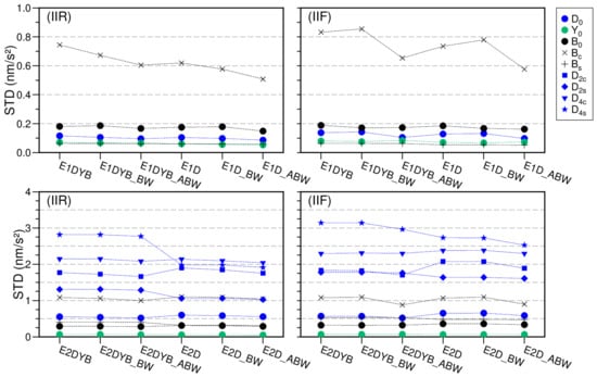
Figure 6.
Standard deviation (STD) of SRP coefficient time series for eclipsing satellites in the 12 solutions. Upper panels: ECOM1 empirical SRP modeling; lower panels: ECOM2 empirical SRP modeling; left panels: GPS BLOCK IIR satellites; right panels: GPS BLOCK IIF satellites. Note the different y-axis scales between the upper and lower panels.
Summarizing the sensitivity of the GPS BLOCK IIR and IIF satellites to the accelerations in the direction of Y and B, they both suffer from the accelerations in the Y direction, which is independent on angle, whereas the BLOCK IIF satellites show smaller accelerations. The visible changes during eclipse seasons for the BLOCK IIR satellites may be caused by the active thermal control before and after the middle of an eclipse event and can be removed mostly by considering additional accelerations in the X surfaces. The dependence of the accelerations in the B direction on angle is caused not only by SRP but also by other nonconservative forces, such as the thermal radiation, as mentioned in Section 2. Applying an a priori box-wing or adjustable box-wing model will improve the stability (STD values) of periodic terms (for instance, ) but not for the BLOFK IIF satellites. Compared with using Equation (8), using Equation (9) has a positive effect on the stability of periodic terms, especially for the term of the BLOCK IIR satellites. Note that nonconservative force modeling is beyond the scope of this study; therefore, we only focus on the performance of SRP modeling combined with shadow factor.
4.2. Day Boundary Discontinuity of Satellite Orbits
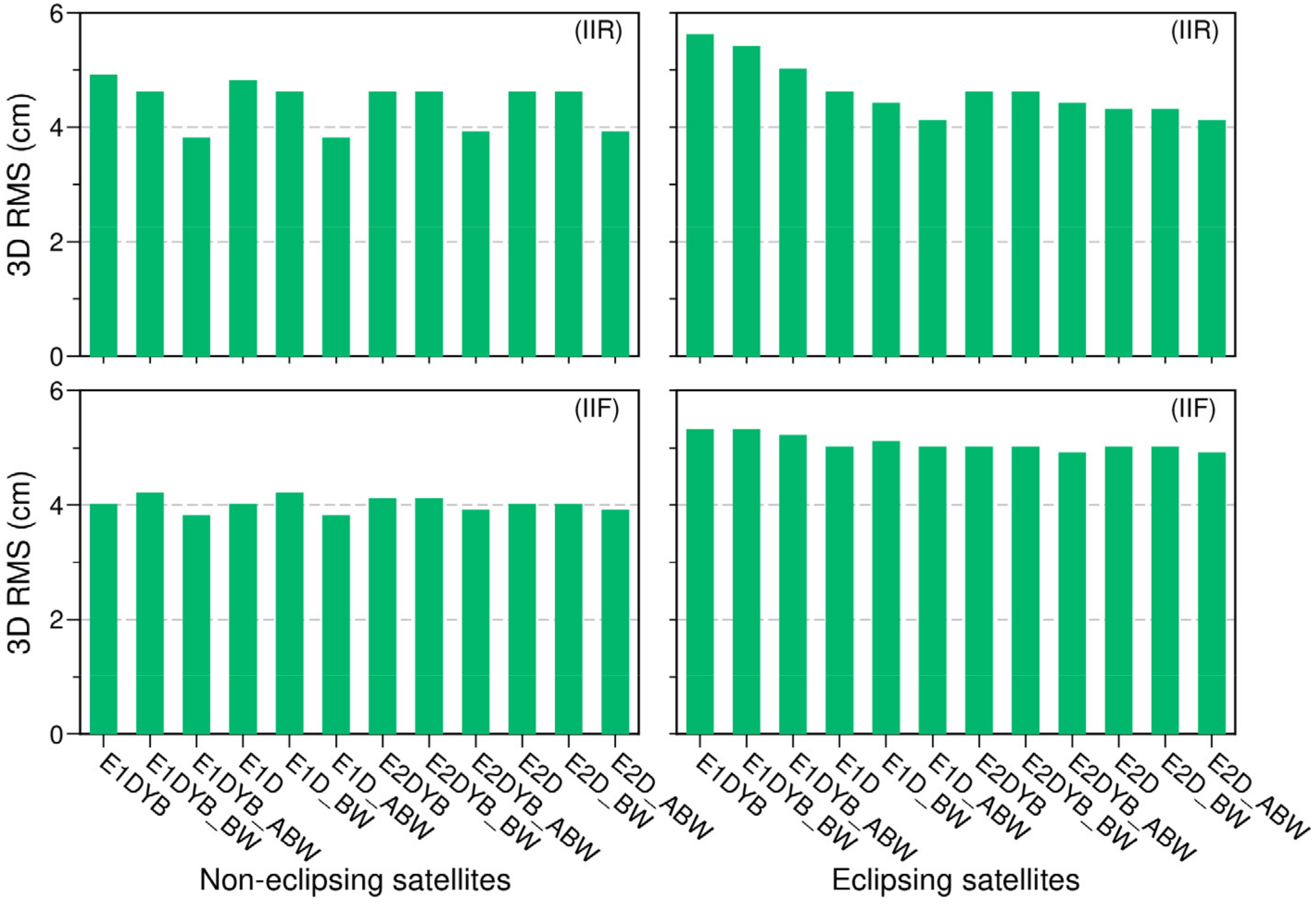
The mean 3D RMS values of orbit DBD for the BLOCK IIR and IIF satellites in different solutions are shown in Figure 7. The method using ECOM2 as a parameterization model (the E2DYB solution) has slightly improved orbit precision in eclipse seasons compared to that using ECOM1, especially for the BLOCK IIR satellites. Using the box-wing as an a priori model (the E1DYB_BW solution) slightly improves the orbit precision for BLOCK IIR satellites and using the adjustable box-wing as an a priori model (the E1DYB_ABW solution) further improves the orbit quality for both the BLOCK IIR and IIF satellites, in and out of eclipse seasons. By comparing each pair of solutions between the shadow factor applied in the D direction and that in the DYB directions, for instance, between the E1DYB and E1D solutions, and also between the E1DYB_ABW and E1D_ABW solutions, we can see that eclipsing satellites have smaller RMS values of DBD in latter solutions with the shadow factor applied only in the D direction. A slight improvement for noneclipsing satellites can also be observed when the shadow factor is applied in the D direction of ECOM2, which can be explained by the stability improvement of higher periodic terms ( or ) in Figure 6.
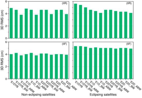
Figure 7.
Mean 3D RMS of day boundary discontinuities in the 12 types of GPS daily precise orbit determination solutions spanning from 2017 to 2019. Upper panels: GPS BLOCK IIR satellites, and lower panels: GPS BLOCK IIF satellites. Left panels: satellites in noneclipsing seasons; right panels: satellites in eclipsing seasons.
For the BLOCK IIR satellites, the orbit precision of E1DYB_ABW and E2DYB_ABW, in which ECOM1 or ECOM2 parameterization model is combined with the a priori adjustable box-wing model and the shadow factor is applied in the D direction, is better than 4 cm for of the noneclipsing satellites, and close to 4 cm for eclipsing satellites. As for the BLOCK IIF satellites, using the adjustable box-wing as an a priori model slightly improves the orbit precision, whereas using the box-wing degrades the orbit precision. Therefore, the solutions using the box-wing model are not discussed in the following analysis.
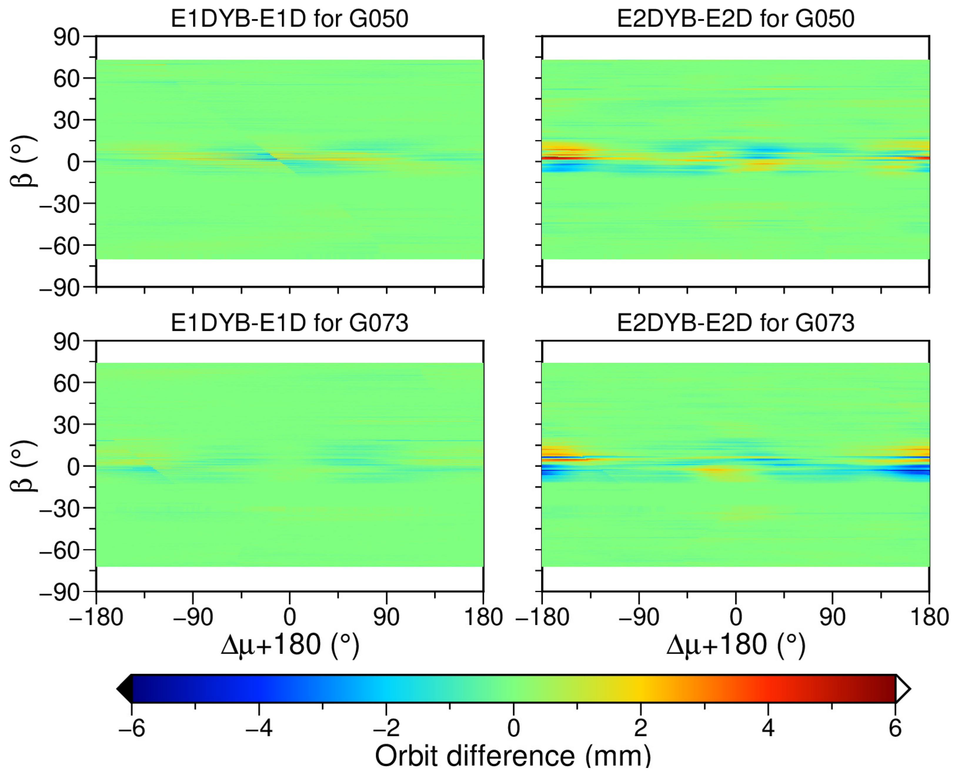
Taking SVN G050 (BLOCK IIR) and SVN G073 (BLOCK IIF) as an example, Figure 8 presents the radial orbit differences between solutions with the shadow factor applied in the D direction and those in the DYB directions. The along and cross components are not given here because the satellite–Sun direction and radial direction of a satellite are close to collinearity when the satellite enters the eclipse season for lower angle. As shown in Figure 8, orbit differences between two methods of using the shadow factor are observed at lower angle, in which the differences based on ECOM2 are more visible. When is around (), that is, the orbit noon, the orbit differences are negative at lower negative angle and positive at lower positive angle. Note that BLOCK IIF satellites show a more visible pattern than BLOCK IIR satellites because of the higher periodic terms in the D direction.
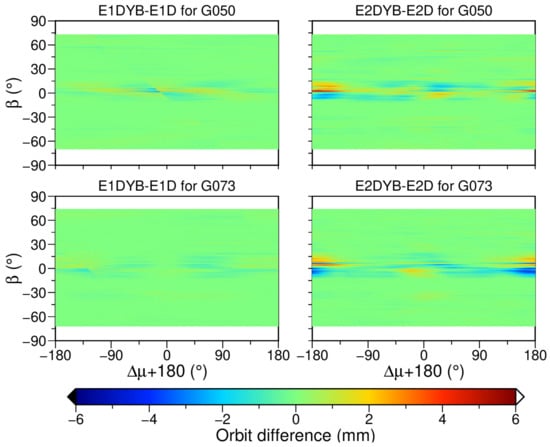
Figure 8.
Differences of satellite orbits in the radial component caused by applying the shadow factor in the D and DYB directions for SVN G050 (BLOCK IIR, upper panels) and G073 (BLOCK IIF, lower panels) as a function of and angle in 2019. is the angular argument. Left and right: using ECOM1 and ECOM2 as parameterization SRP models, respectively.
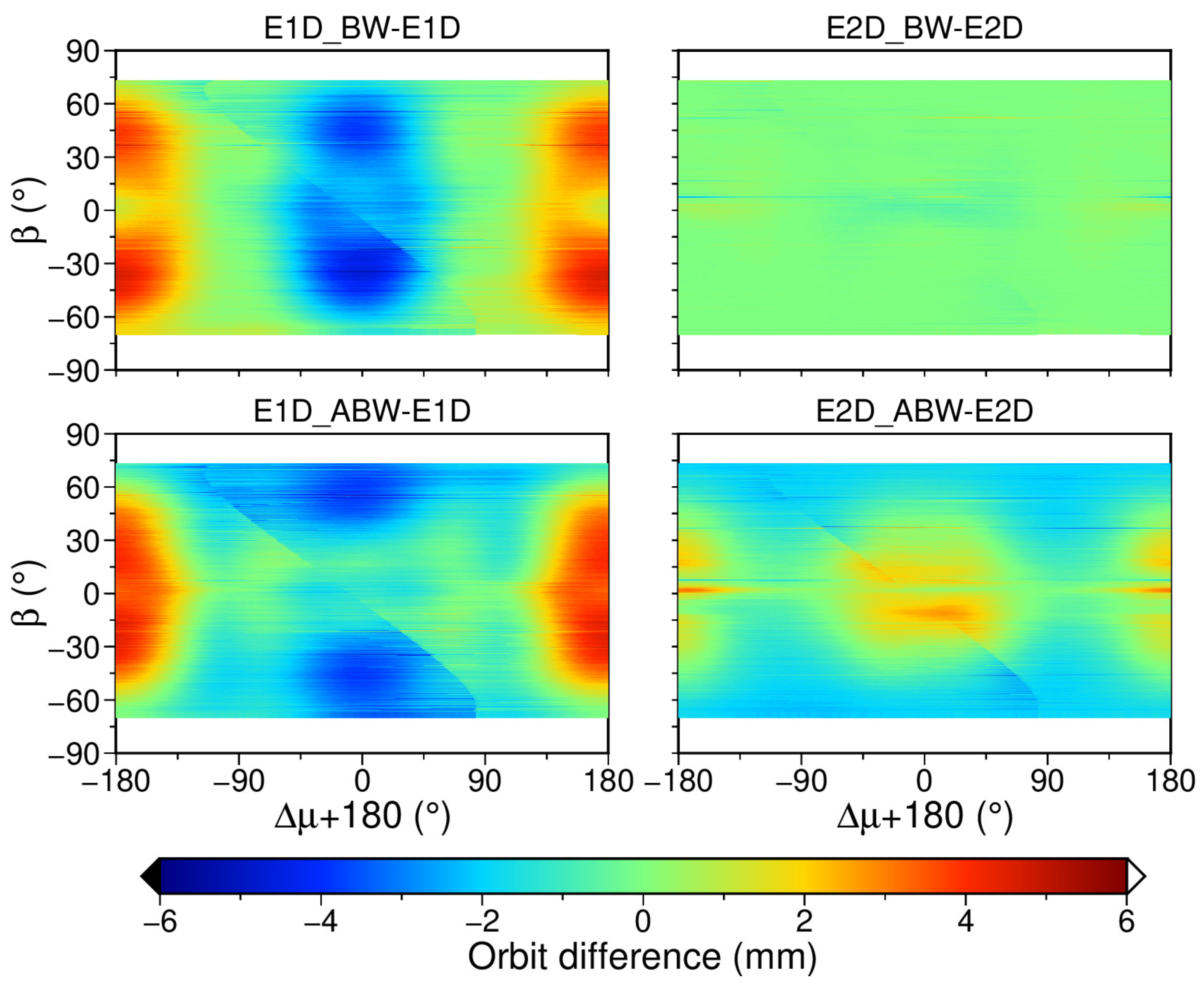
Moreover, the radial orbit differences between using different a priori SRP models are investigated in Figure 9 and Figure 10, which can illustrate the impact of different a priori models on radial orbit. For the GPS SVN050 satellite (BLOCK IIR) shown in Figure 9, using the box-wing or adjustable box-wing as a priori model with the ECOM1 as parameterization model leads to the visible peanutlike distribution of the orbit differences, where the differences can be up to ±6 mm. This pattern is likely owing to the variation of effective illuminated area in the direction (pointing to Earth). Large antenna arrays, namely W-sensor, are installed in surfaces of BLOCK IIR satellites, which cannot be modeled by only one constant parameter in the D direction. The differences shown in the left panel of Figure 9 are reduced when using ECOM2 as parameterization model, especially between box-wing model and no a priori model, indicating that the box-wing as a priori model does not contribute that much when ECOM2 is used as parameterization model.
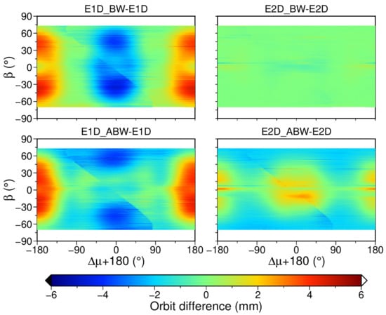
Figure 9.
Differences of satellite orbit in the radial component between solutions using different a priori models for SVN G050 (BLOCK IIR) as a function of and angle in 2019. is the angular argument. Upper: differences between using no a priori SRP model and using the box-wing model; lower: differences between using no a priori SRP model and using the adjustable box-wing model. Left and right panels: using the ECOM1 and ECOM2 as the parameterization model, respectively.
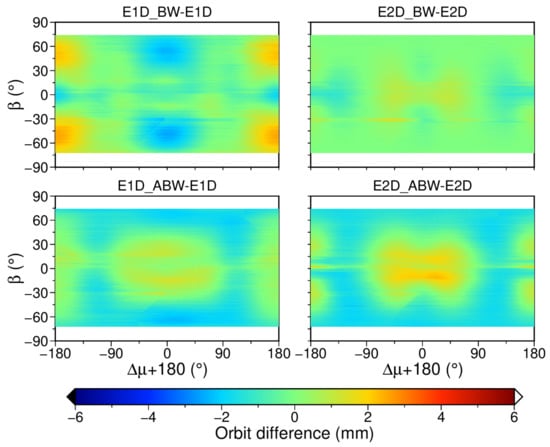
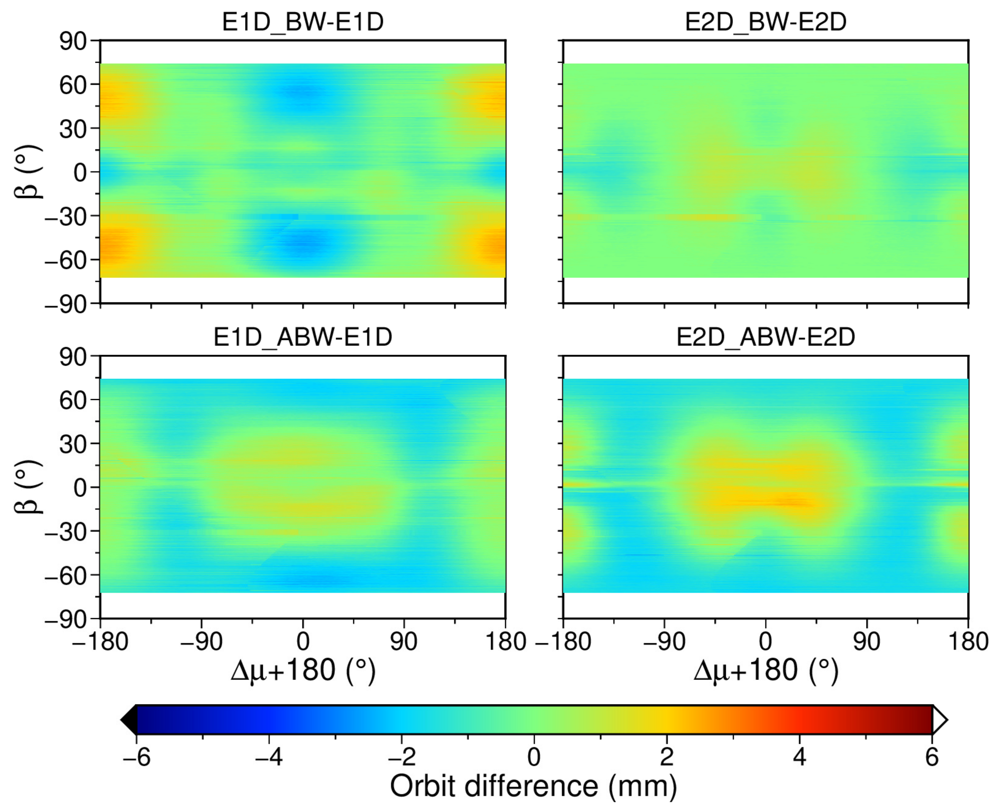
Figure 10.
Differences of satellite orbits in the radial component between different a priori models for G073 (BLOCK IIF) as a function of and angle in 2019. is the angular argument. Upper: differences between using no a priori SRP model and using the box-wing model; lower: differences between using no a priori SRP model and using the adjustable box-wing model. Left and right panels: using ECOM1 and ECOM2 as parameterization model, respectively.
In addition to the BLOCK IIR satellites, the orbit radial differences of the BLOCK IIF satellites (SVN G073) are further investigated in Figure 10. As it is shown, the differences caused by applying a priori box-wing model are largely reduced compared with corresponding results of BLOCK IIR satellites shown in Figure 9. Note that when using the ECOM2 as parameterization model, the visible differences at lower angle between with and without an a priori adjustable box-wing model may be related to the adjustment of shape value in the adjustable box-wing modeling [8].
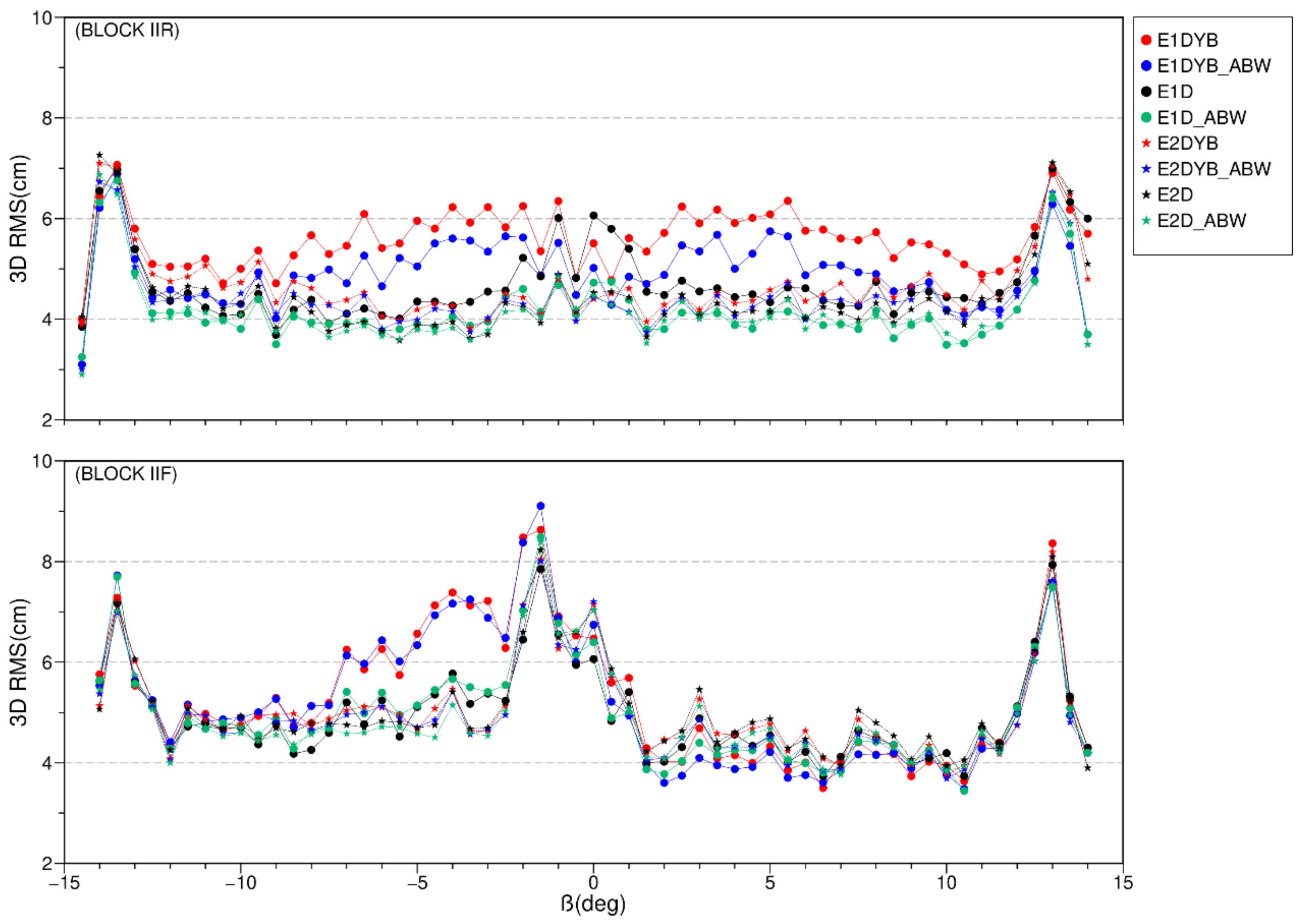
Due to fact that current box-wing model has a little improvement on BLOCK IIR satellite orbit precision, even a negative effect on BLOCK IIF satellites, we focus on the evaluation of adjustable box-wing model and the methods of applying the shadow factor. The 3D RMS values of DBD with respect to angle for eclipsing satellites in different solutions are shown in Figure 11. For BLOCK IIR satellites shown in the upper panel, RMS values of DBD in E1DYB (red dot) and E1DYB_ABW (blue dot) solutions increase with declining during the eclipse period. Applying the shadow factor only in the D direction removes the rising trend mostly for , that is, the E1D (black dot) and E1D_ABW (green dot) solutions. However, in the E1D solution, the RMS values still increase in the case of lower β angle, that is, . By using the ECOM2 instead of the ECOM1 and applying the shadow factor in the D direction, the RMS values are reduced to a large extent. Note the relatively larger RMS values of DBD up to 6–8 cm for both BLOCK IIR and BLOCK IIF satellites at the beginning of eclipse events, that is, .
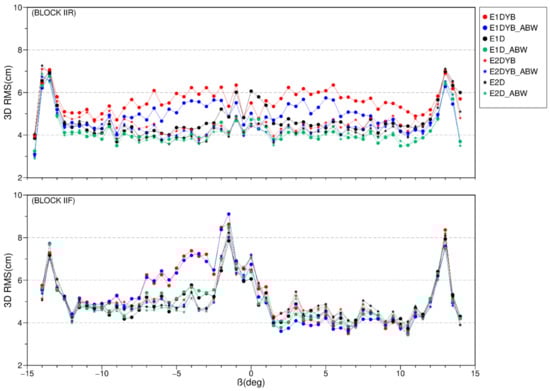
Figure 11.
3D RMS values of DBD for BLOCK IIR (upper panel) and BLOCK IIF (lower panel) in eclipse seasons with respect to the angle spanning from 2017 to 2019. Note that there is no difference between using no a priori SRP model and using the box-wing model; the solutions using the box-wing model are thus not presented.
For the BLOCK IIF satellites shown in the lower panel of Figure 11, an asymmetrical pattern is observed between negative and positive angles, which is similar with the SRP coefficients variation in Section 4.1 (see Figure 4 and Figure 5). All solutions have small orbit differences with each other when the angle is positive, including the E1DYB and E1DYB_ABW solutions. The large RMS values are also observed for BLOCK IIF satellites at transition from full phase to umbra or inverse. This phenomenon also needs further investigation.
Further statistics of the RMS values of DBD in the along, cross, and radial components from 2017 to 2019 are summarized in Table 3. The solutions with shadow factor applied in the D direction are generally better that those with shadow factor applied in the DYB directions, especially for the cross and radial components. For the BLOCK IIR satellites in eclipse seasons, the RMS values of DBD are reduced from 2.8 cm and 3.1 cm in the E1DYB solution to 2.1 cm and 2.4 cm in the E1D solution in the cross and radial directions, respectively. For the BLOCK IIF satellites in eclipse seasons, the improvement from the E1DYB to E1D solution is only 0.4 cm in the radial direction, and that in the along and cross directions are neglectable. When an adjustable box-wing model is used, we can see the orbit improvement in and out of eclipse seasons, and the improvement of the BLOCK IIR satellites are larger than that of BLOCK IIF satellites. The orbits are further improved when applying the shadow factor in the D direction and using the adjustable box-wing model as a priori SPR model simultaneously, that is, the E1D_ABW and E2D_ABW solutions. The values of E1D_ABW solution for BLOCK IIR satellites out of eclipse seasons are 2.3 cm, 1.7 cm, and 1.7 cm in the along, cross, and radial directions, respectively, and the corresponding values in eclipse seasons are 2.5 cm, 2.4 cm, and 2.7 cm. Moreover, the DBD of the E1D_ABW solution has a comparable accuracy with the E2D_ABW solution.
Table 3.
RMS values of the orbit DBD in 2017–2019. We distinguish between statistics in and out of eclipse seasons for both BLOCK IIR and BLOCK IIF satellites. A stands for the along direction, C stands for the cross direction, and R stands for the radial direction. The unit is cm. Note that there is no difference between using no a priori SRP model and using the box-wing model; the solutions using the box-wing model are thus not presented.
4.3. Impact on the Earth Rotation Parameters
In addition to the performance of satellite orbit precision, the ERP components are also sensitive to the satellite orbit dynamic modeling [51]. The ERP component estimations of different solutions are compared to the IERS EOP 14C04 product [48] and the WSTD values are given in Table 4. The different methods of modeling SRP and applying the shadow factor have an insignificant impact on the ERP agreement with the IERS product, and the WSTD of each solution is around 43.6 to 44.7 μas, 23.1 to 24.8 μas, 213.2 to 216.0 μas/day, and 8.7 to 9.8 μs/day for the x-pole, y-pole, x-pole rate, and LoD components, respectively. As for the y-pole rate, however, using the adjustable box-wing as an a priori SRP model clearly improves the precision—for instance, with the WSTD value reduced from 205.3 μas/day in solution E1DYB to 184.9 μas/day in solution E1DYB_ABW. The impact of using ECOM1 or ECOM2 models and that of applying the shadow factor in the D or DYB directions on y-pole rate precision are rather diverse. There is insignificant difference between applying the shadow factor in the D direction and in the DYB directions for the polar motion offset and rate, whereas the LoD always shows an improved precision when the shadow factor applied in the D direction. Moreover, the E1D_ABW solution has the smallest WSTD of the LoD (8.7 μs/day), which is improved by about 8% compared with the E2DYB_ABW solution (9.7 μs/day).
Table 4.
WSTD values of the ERP differences between GPS precise orbit determination solutions and the IERS EOP 14C04 product. Note that there is no difference between using no a priori SRP model and using the box-wing model; the solutions using the box-wing model are thus not presented.
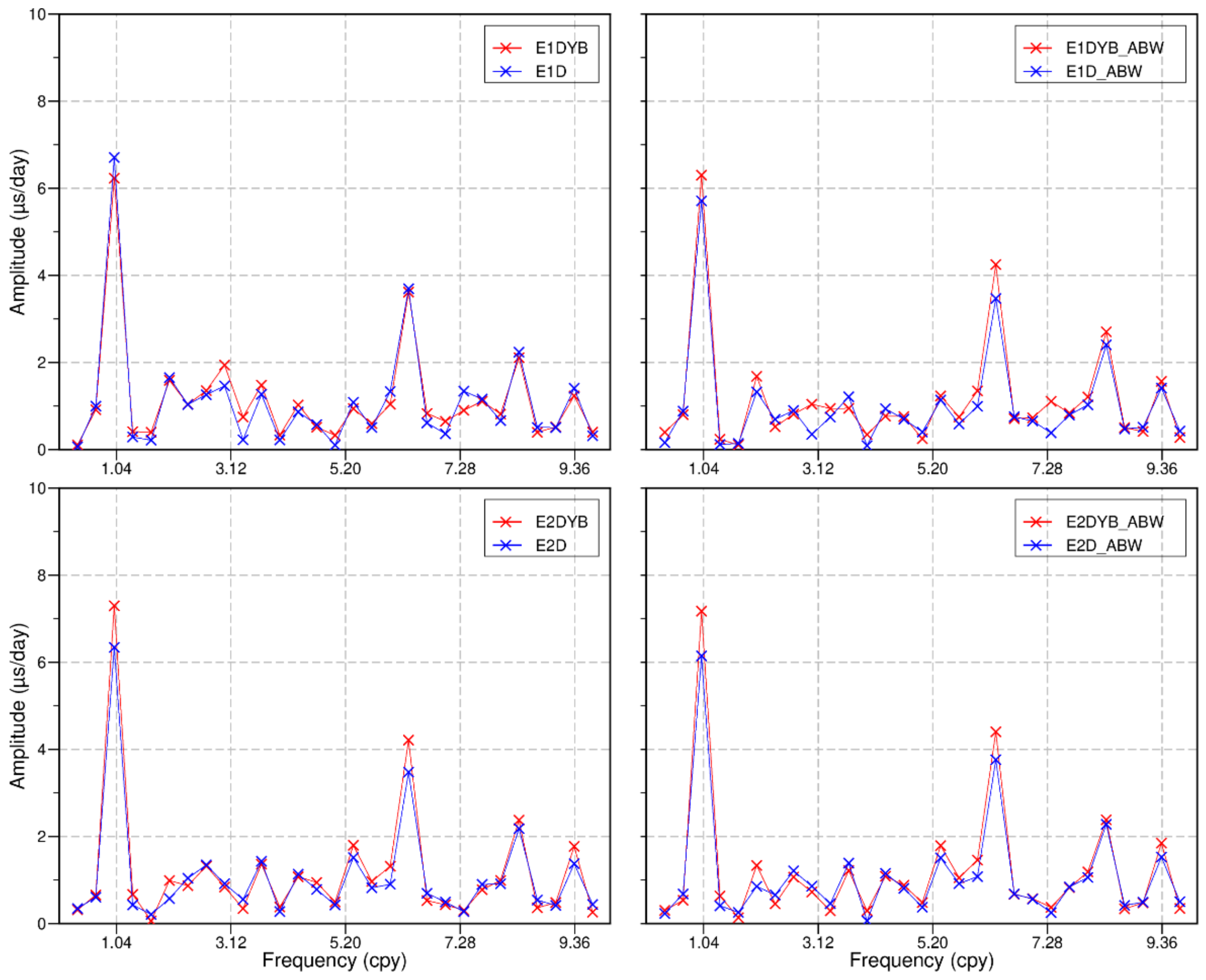
Figure 12 further presents the power spectra of the LoD in eight solutions, which demonstrates the impact of the SRP modeling. A clear reduction in the 1.04 cpy and 6.30 cpy signals is observed when applying the shadow factor in the D instead of the DYB directions. The only exception is when using the pure ECOM1 parameterization model without an a priori model, that is, between E1DYB and E1D, where the 1.04 cpy signal is larger in the E1D solution than in the E1DYB solution.
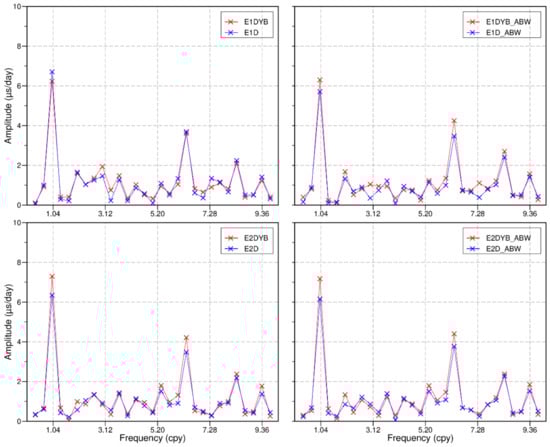
Figure 12.
Power spectra of the LoD differences with respect to the IERS EOP 14C04 product. Upper panels: ECOM1 for the empirical SRP modeling, lower panels: ECOM2 for the empirical SRP modeling; left panels: no a priori SRP modeling, right panels: adjustable box-wing for the a priori SRP modeling.
5. Conclusions
In this study, we investigated the performance of different SRP models, including the box-wing and adjustable box-wing as the a priori model, and the ECOM1 and ECOM2 as the parameterization model in GPS POD solutions. We paid special attention to the orbit behavior during eclipse seasons, focusing on the two methods of handling the shadow factor, that is, applying in either the D or the D, Y, and B directions. We processed the daily GPS POD solution using three years of observations and evaluated the results in terms of the SRP coefficients, the day boundary discontinuity values of orbits, and the ERP agreement to the IERS EOP 14C04.
For the GPS BLOCK IIR satellite, the performance of the SRP coefficient between in and out of eclipse seasons is consistent with the shadow factor that is applied in the D direction but rather diverse when applied in the DYB directions. The diversity of the coefficient in and out of eclipse seasons is possibly stemming from nonconservative forces in surfaces, e.g., radiator. A notable discrepancy in the behavior of for the BLOCK IIR and BOCK IIF satellites is probably related to the difference in satellite design, thermal control model, etc., which needs further investigation in the future. For the coefficients in the B direction, its dependency on angle is caused not only by SRP but also by other unmodeled non-SRP forces, which can partly be absorbed by the once-per-revolution terms in ECOM1 and ECOM2. Moreover, applying a priori box-wing or adjustable box-wing model can improve the stability of periodic terms in terms of the standard deviation, especially for the and terms in the D direction because of the parameters’ correlation, except for the BLOCK IIF satellites using the a priori box-wing model. Among all solutions, the one combining a priori adjustable box-wing with ECOM1 with the shadow factor applied in the D direction (that is, the E1D_AWB) has the best SRP coefficient stability with the smallest STD values.
We also demonstrated that using the a priori adjustable box-wing model and applying the shadow factor in the D instead of the DYB directions both can improve the orbit quality, especially in the cross and radial directions. Compared with the E1DYB solution using no a priori SRP and the shadow factor applied in the DYB directions, the RMS values of orbit DBD in the E1D_ABW solution (using a priori adjustable box-wing model with shadow factor applied in the D direction) are improved by 7.7%, 32.1%, and 35.5% for the BLOCK IIR satellites in noneclipsing seasons in the along, cross, and radial direction, respectively, and the corresponding improvements in the eclipse season are 17.8%, 22.7%, and 26.1%. In the E1D_ABW or E2D_ABW solution, the BLOCK IIR satellites show similar behavior in and out of eclipse seasons. As for the ERP agreement to the IERS EOP 14C04, the LoD is improved when the shadow factor is applied in the D direction instead of the DYB directions. The reason of the deteriorated performance of SRP coefficients and DBD values for the BLOCK IIF satellites when applying box-wing model can be attributed to the fact that the shape and optical properties were collected directly from some documents, which might not be accurate enough.
The analyses in this study provide a verification for the presence of unmodeled thermal effects in GPS satellites [8,33]. Although applying the shadow factor only in the D direction during eclipse seasons can absorb some nonconservative forces, some orbit modeling deficiencies still exist, especially for the BLOCK IIF satellites. A further consideration of unmodeled forces (such as thermal radiator, heating, or cooling of surfaces) in each surface will contribute to establishing a more precise SRP model to improve satellite orbits, especially in eclipse seasons.
Author Contributions
L.T. conceived the idea and designed the experiments with M.G. and J.W., L.T. and J.W. wrote the main manuscript. H.S., A.X., M.G., H.Z. and J.W. reviewed the paper. All components of this research were carried out under the supervision of L.T. and M.G. All authors have read and agreed to the published version of the manuscript.
Funding
This research was funded by the National Natural Science Foundation of China (Grant Nos. 42030109, 42074012), The Liaoning Key Research and Development Program (No. 2020JH2/10100044), and The National Key Research and Development Program (No. 2016YFC0803102). L.T. is financially supported by the China Scholarship Council (CSC, Files 201908210371).
Institutional Review Board Statement
Not applicable.
Informed Consent Statement
Not applicable.
Data Availability Statement
Not applicable.
Acknowledgments
This work is based on the GPS observations provided by IGS. We would like to thank the data lefts and related agencies and organizations. All calculations are conducted based on the Positioning And Navigation Data Analyst (PANDA) software. The authors also would like to thank the anonymous reviewers for their effort and valuable comments to the manuscript.
Conflicts of Interest
The authors declare no conflict of interest.
References
- Altamimi, Z.; Rebischung, P.; Métivier, L.; Collilieux, X. ITRF2014: A new release of the International Terrestrial Reference Frame modeling nonlinear station motions. J. Geophys. Res. Solid Earth 2016, 121, 6109–6131. [Google Scholar] [CrossRef] [Green Version]
- Sośnica, K.; Bury, G.; Zajdel, R.; Strugarek, D.; Drożdżewski, M.; Kazmierski, K. Estimating global geodetic parameters using SLR observations to Galileo, GLONASS, BeiDou, GPS, and QZSS. Earth Planets Space 2019, 71, 20. [Google Scholar] [CrossRef] [Green Version]
- Argus, D.F.; Heflin, M.B. Plate motion and crustal deformation estimated with geodetic data from the Global Positioning System. Geophys. Res. Lett. 1995, 22, 1973–1976. [Google Scholar] [CrossRef]
- Calais, E.; Han, J.-Y.; DeMets, C.; Nocquet, J.-M. Deformation of the North American plate interior from a decade of continuous GPS measurements. J. Geophys. Res. Space Phys. 2006, 111, B06402. [Google Scholar] [CrossRef] [Green Version]
- Wang, J.; Wu, Z.; Semmling, M.; Zus, F.; Gerland, S.; Ramatschi, M.; Ge, M.; Wickert, J.; Schuh, H. Retrieving Precipitable Water Vapor From Shipborne Multi-GNSS Observations. Geophys. Res. Lett. 2019, 46, 5000–5008. [Google Scholar] [CrossRef] [Green Version]
- Wu, Z.; Liu, Y.; Liu, Y.; Wang, J.; He, X.; Xu, W.; Ge, M.; Schuh, H. Validating HY-2A CMR precipitable water vapor using ground-based and shipborne GNSS observations. Atmos. Meas. Tech. 2020, 13, 4963–4972. [Google Scholar] [CrossRef]
- Griffiths, J. Combined orbits and clocks from IGS second reprocessing. J. Geod. 2019, 93, 177–195. [Google Scholar] [CrossRef] [PubMed] [Green Version]
- Duan, B.; Hugentobler, U. Enhanced solar radiation pressure model for GPS satellites considering various physical effects. GPS Solut. 2021, 25, 1–14. [Google Scholar] [CrossRef]
- Kouba, J. A simplified yaw-attitude model for eclipsing GPS satellites. GPS Solut. 2009, 13, 1–12. [Google Scholar] [CrossRef]
- Fliegel, H.F.; Gallini, T.E.; Swift, E.R. Global Positioning System Radiation Force Model for geodetic applications. J. Geophys. Res. Space Phys. 1992, 97, 559. [Google Scholar] [CrossRef]
- Fliegel, H.F.; Gallini, T.E. Solar force modeling of block IIR Global Positioning System satellites. J. Spacecr. Rocket. 1996, 33, 863–866. [Google Scholar] [CrossRef]
- Rodriguez-Solano, C.J. Impact of Non-Conservative Force Modelling on GNSS Satellite Orbits and Global Solutions. Ph.D. Dissertation, Technische Universität München, Munich, Germany, 2014. [Google Scholar]
- Rodriguez-Solano, C.; Hugentobler, U.; Steigenberger, P. Adjustable box-wing model for solar radiation pressure impacting GPS satellites. Adv. Space Res. 2012, 49, 1113–1128. [Google Scholar] [CrossRef]
- Fliegel, H.; Feess, W.; Layton, W.; Rhodus, N. The GPS radiation Force Model. In Proceedings of the 1st International Symposium on Precise Positioning with the Global Positioning System, Rockville, MA, USA, 15–19 April 1985. [Google Scholar]
- Fliegel, H. Radiation pressure models for Block II GPS satellites. In Proceedings of the Fifth International Geodetic Symposium on Satellite Positioning, Las Cruces, NM, USA, 13–17 March 1989; pp. 789–798. [Google Scholar]
- Bar-Sever, Y.; Kuang, D. New empirically derived solar radiation pressure model for global positioning system satellites during eclipse seasons. IPN Prog. Rep. 2005, 1, 42–160. [Google Scholar]
- Beutler, G.; Brockmann, E.; Gurtner, W.; Hugentobler, U.; Mervart, L.; Rothacher, M.; Verdun, A. Extended orbit modeling techniques at the CODE processing center of the international GPS service for geodynamics (IGS): Theory and initial results. Manuscr. Geod. 1994, 19, 367–386. [Google Scholar]
- Springer, T.A.; Beutler, G.; Rothacher, M. A New Solar Radiation Pressure Model for GPS Satellites. GPS Solut. 1999, 2, 50–62. [Google Scholar] [CrossRef]
- Arnold, D.; Meindl, M.; Beutler, G.; Dach, R.; Schaer, S.; Lutz, S.; Prange, L.; Sośnica, K.; Mervart, L.; Jäggi, A. CODE’s new solar radiation pressure model for GNSS orbit determination. J. Geod. 2015, 89, 775–791. [Google Scholar] [CrossRef] [Green Version]
- Prange, L.; Villiger, A.; Sidorov, D.; Schaer, S.; Beutler, G.; Dach, R.; Jäggi, A. Overview of CODE’s MGEX solution with the focus on Galileo. Adv. Space Res. 2020, 66, 2786–2798. [Google Scholar] [CrossRef]
- Deng, Z.; Nischan, T.; Bradke, M. Multi-GNSS Rapid Orbit-, Clock- & EOP-Product Series; GFZ Data Services: Potsdam, Germany, 2017. [Google Scholar]
- Guo, J.; Xu, X.; Zhao, Q.; Liu, J. Precise orbit determination for quad-constellation satellites at Wuhan University: Strategy, result validation, and comparison. J. Geod. 2016, 90, 143–159. [Google Scholar] [CrossRef]
- Rodriguez-Solano, C.J.; Hugentobler, U.; Steigenberger, P.; Blosfeld, M.; Fritsche, M. Reducing the draconitic errors in GNSS geodetic products. J. Geod. 2014, 88, 559–574. [Google Scholar] [CrossRef]
- Meindl, M.; Beutler, G.; Thaller, D.; Dach, R.; Jäggi, A. Geocenter coordinates estimated from GNSS data as viewed by perturbation theory. Adv. Space Res. 2013, 51, 1047–1064. [Google Scholar] [CrossRef]
- Montenbruck, O.; Steigenberger, P.; Hugentobler, U. Enhanced solar radiation pressure modeling for Galileo satellites. Bull. Géod. 2014, 89, 283–297. [Google Scholar] [CrossRef]
- Steigenberger, P.; Montenbruck, O.; Hugentobler, U. GIOVE-B solar radiation pressure modeling for precise orbit determination. Adv. Space Res. 2014, 55, 1422–1431. [Google Scholar] [CrossRef]
- Bury, G.; Zajdel, R.; Sośnica, K. Accounting for perturbing forces acting on Galileo using a box-wing model. GPS Solut. 2019, 23, 1–12. [Google Scholar] [CrossRef] [Green Version]
- Li, X.; Yuan, Y.; Huang, J.; Zhu, Y.; Wu, J.; Xiong, Y.; Li, X.; Zhang, K. Galileo and QZSS precise orbit and clock determination using new satellite metadata. J. Geod. 2019, 93, 1123–1136. [Google Scholar] [CrossRef]
- Sibthorpe, A.; Bertiger, W.; Desai, S.D.; Haines, B.; Harvey, N.; Weiss, J.P. An evaluation of solar radiation pressure strategies for the GPS constellation. J. Geod. 2011, 85, 505–517. [Google Scholar] [CrossRef]
- Chang, X.; Männel, B.; Schuh, H. An analysis of a priori and empirical solar radiation pressure models for GPS satellites. Adv. Geosci. 2021, 55, 33–45. [Google Scholar] [CrossRef]
- Liu, Y.; Liu, Y.; Tian, Z.; Dai, X.; Qing, Y.; Li, M. Impact of ECOM Solar Radiation Pressure Models on Multi-GNSS Ultra-Rapid Orbit Determination. Remote Sens. 2019, 11, 3024. [Google Scholar] [CrossRef] [Green Version]
- Guo, J.; Chen, G.; Zhao, Q.; Liu, J.; Liu, X. Comparison of solar radiation pressure models for BDS IGSO and MEO satellites with emphasis on improving orbit quality. GPS Solut. 2017, 21, 511–522. [Google Scholar] [CrossRef] [Green Version]
- Sidorov, D.; Dach, R.; Polle, B.; Prange, L.; Jäggi, A. Adopting the empirical CODE orbit model to Galileo satellites. Adv. Space Res. 2020, 66, 2799–2811. [Google Scholar] [CrossRef]
- Montenbruck, O.; Schmid, R.; Mercier, F.; Steigenberger, P.; Noll, C.; Fatkulin, R.; Kogure, S.; Ganeshan, A. GNSS satellite geometry and attitude models. Adv. Space Res. 2015, 56, 1015–1029. [Google Scholar] [CrossRef] [Green Version]
- Montenbruck, O.; Gill, E.; Lutze, F. Satellite Orbits: Models, Methods, and Applications. Appl. Mech. Rev. 2002, 55, B27–B28. [Google Scholar] [CrossRef]
- Marquis, W.; Krier, C. Examination of the GPS block IIR solar pressure model. In Proceedings of the 13th International Technical Meeting of the Satellite Division of The Institute of Navigation (ION GPS 2000), Salt Lake City, UT, USA, September 19–22 2000; pp. 407–415. [Google Scholar]
- Liu, J.; Ge, M. PANDA software and its preliminary result of positioning and orbit determination. Wuhan Univ. J. Nat. Sci. 2003, 8, 603. [Google Scholar]
- Bar-Sever, Y.E. A new model for GPS yaw attitude. J. Geod. 1996, 70, 714–723. [Google Scholar] [CrossRef]
- Dilssner, F.; Springer, T.; Enderle, W. GPS IIF yaw attitude control during eclipse season. In Proceedings of the AGU Fall Meeting Abstracts, San Francisco, CA, USA, 5–9 December 2011. [Google Scholar]
- Kuang, D.; Desai, S.; Sibois, A. Observed features of GPS Block IIF satellite yaw maneuvers and corresponding modeling. GPS Solut. 2017, 21, 739–745. [Google Scholar] [CrossRef]
- Petit, G.; Luzum, B. IERS Conventions (2010); Bureau International des Poids et Mesures: Sevres, France, 2010. [Google Scholar]
- Böhm, J.; Moeller, G.; Schindelegger, M.; Pain, G.; Weber, R. Development of an improved empirical model for slant delays in the troposphere (GPT2w). GPS Solut. 2015, 19, 433–441. [Google Scholar] [CrossRef] [Green Version]
- Boehm, J.; Niell, A.; Tregoning, P.; Schuh, H. Global Mapping Function (GMF): A new empirical mapping function based on numerical weather model data. Geophys. Res. Lett. 2006, 33, 33. [Google Scholar] [CrossRef] [Green Version]
- Chen, G.; Herring, T. Effects of atmospheric azimuthal asymmetry on the analysis of space geodetic data. J. Geophys. Res. Space Phys. 1997, 102, 20489–20502. [Google Scholar] [CrossRef]
- Ge, M.; Gendt, G.; Dick, G.; Zhang, F.P. Improving carrier-phase ambiguity resolution in global GPS network solutions. J. Geod. 2005, 79, 103–110. [Google Scholar] [CrossRef]
- Ge, M.; Gendt, G.; Dick, G.; Zhang, F.P.; Rothacher, M. A New Data Processing Strategy for Huge GNSS Global Networks. J. Geod. 2006, 80, 199–203. [Google Scholar] [CrossRef]
- Sośnica, K.; Thaller, D.; Dach, R.; Steigenberger, P.; Beutler, G.; Arnold, D.; Jaggi, A. Satellite laser ranging to GPS and GLONASS. J. Geod. 2015, 89, 725–743. [Google Scholar] [CrossRef] [Green Version]
- Bizouard, C.; Lambert, S.; Gattano, C.; Becker, O.; Richard, J.-Y. The IERS EOP 14C04 solution for Earth orientation parameters consistent with ITRF 2014. J. Geod. 2019, 93, 621–633. [Google Scholar] [CrossRef]
- Rodriguez-Solano, C.; Hugentobler, U.; Steigenberger, P.; Allende-Alba, G. Improving the orbits of GPS block IIA satellites during eclipse seasons. Adv. Space Res. 2013, 52, 1511–1529. [Google Scholar] [CrossRef]
- Bury, G.; Sośnica, K.; Zajdel, R.; Strugarek, D. Toward the 1-cm Galileo orbits: Challenges in modeling of perturbing forces. J. Geod. 2020, 94, 16. [Google Scholar] [CrossRef] [Green Version]
- Rothacher, M.; Beutler, G.; Herring, T.; Weber, R. Estimation of nutation using the Global Positioning System. J. Geophys. Res. Space Phys. 1999, 104, 4835–4859. [Google Scholar] [CrossRef]


Publisher’s Note: MDPI stays neutral with regard to jurisdictional claims in published maps and institutional affiliations. |
© 2021 by the authors. Licensee MDPI, Basel, Switzerland. This article is an open access article distributed under the terms and conditions of the Creative Commons Attribution (CC BY) license (https://creativecommons.org/licenses/by/4.0/).