Abstract
The efficiency of a vineyard management system is directly related to the effective management of nutritional disorders, which significantly downgrades vine growth, crop yield and wine quality. To detect nutritional disorders, we successfully extracted a wide range of features using hyperspectral (HS) images to identify healthy and individual nutrient deficiencies of grapevine leaves. Features such as mean reflectance, mean first derivative reflectance, variation index, mean spectral ratio, normalised difference vegetation index (NDVI) and standard deviation (SD) were employed at various stages in the ultraviolet (UV), visible (VIS) and near-infrared (N.I.R.) regions for our experiment. Leaves were examined visually in the laboratory and grouped as either healthy (i.e. control) or unhealthy. Then, the features of the leaves were extracted from these two groups. In a second experiment, features of individual nutrient-deficient leaves (e.g., N, K and Mg) were also analysed and compared with those of control leaves. Furthermore, a customised support vector machine (SVM) was used to demonstrate that these features can be utilised with a high degree of effectiveness to identify unhealthy samples and not only to distinguish from control and nutrient deficient but also to identify individual nutrient defects. Therefore, the proposed work corroborated that HS imaging has excellent potential to analyse features based on healthiness and individual nutrient deficiencies of grapevine leaves.
1. Introduction
Hyperspectral (HS) imaging has numerous applications in agricultural research. It is a non-contact and non-destructive approach that collects spectral and spatial information from an object between the UV and IR regions. An extensive volume of information can be generated utilising its high spectral resolution in recognising, classifying and measuring target objects [1,2]. This is a widely used technique to study the quality [3,4,5,6,7,8,9], diseases [10,11] and defects of agricultural products such as fruits and vegetables [12].
HS imaging is also widely used in the viticulture sector and the wine industry. In viticulture, HS imaging is used for determining phenolic contents in wine grapes [13,14], predicting sugar content of grapes [15], for the classification of grapevine varieties under field conditions [16] and modelling water stress in the vineyard [17]. Different diseases [18,19] of grapevine leaves can also be detected with the aid of HS imaging.
Along with other factors such as climate, temperature, light intensity, and water content of grapevine, healthiness and nutrient content of grapevine leaves play essential roles in the production of high quality grapes [18,19,20,21,22,23,24,25,26]. The photosynthesis process produces food for the plant to survive, and it is necessary for the production of sugar, and sugar-based elements in grapes [20]. Diseases such as powdery mildew [22,23], leafroll [18] and red blotch disease [19], etc., are deleterious to the production of high-quality grapes. The macro-nutrients, including nitrogen (N), potassium (K), and magnesium (Mg), are essential elements that impact vine growth, grape yield and wine quality [24,25,26]. Currently, plant tissue or soil sampling, followed up with chemical analysis, informs on whether a nutrient is deficient, adequate, luxurious or in toxic concentrations. Viticulturists can then make informed decisions on the particular soil or plant amendments that are required to correct these inadequacies. Unfortunately, these laboratory analyses are costly, may take several days or weeks to process, and the results can be difficult to interpret. During economic hardship, the frequency of plant tissue or soil analysis may be reduced or even abandoned altogether. This may lead to the inappropriate and/or over-application of fertilisers contributing to environmental issues such as leaching, run-off and increased greenhouse gas emissions. Similarly, the incorrect diagnosis of diseases and pests can lead to the inappropriate application and excessive use of pesticides leading to the contamination of soil, surface and groundwater. Accurate, simple and rapid tools are required so that viticulturists can make timely and cost-effective decisions. HS imaging may be one tool to fill this gap. Studies focused on HS imaging for diseases and nutrient deficiency detection have been conducted on grapevines [18,19,27,28]. N. Bendel et al. [18] presented a hyperspectral-based method where spectral pre-processing in combination with a machine learning model was used to detect leafroll-associated virus 1 and 3 in white and red grapevine cultivars. In this literature, it was reported that the data were obtained from plants that were grown both in control laboratory conditions and in the field during three consecutive years.
H. Al-Saddik et al. [27] applied successive projection algorithms, machine learning such as support vector machine learning and vegetation indices to detect vineyard disease based on hyperspectral data. M. Mehrübeoglu et al. [19] obtained modified reflectance data at 566 nm and 628 nm and modified reflectance ratios computed at 566 nm/628 nm and 680 nm/738 nm. These features were then used to train a support vector machine for detecting red blotch disease in grape leaves. There is no comparison study reported concerning features of visibly healthy relative to unhealthy leaves using HS imaging in order to study individual nutrient deficiencies in grapevines. The study will provide insight into vine performance and decision support tools for improved vineyard management. With this end goal in mind, this research work aims to extract a comprehensive set of features from healthy and nutritional deficient grapevine leaves using an HS camera. In the case of the preliminary healthiness study, the features of visibly unhealthy sample leaves were compared to those that were healthy. For the nutrition deficiency study, features of different nutrient-deficient leaves were compared with those of control leaves which were grown in a controlled environment. Finally, a customised multiclass support vector machine (SVM) technique was used to classify control, unhealthy leaves and individual nutritional disorders (i.e., N, K and Mg). An SVM is a supervised machine learning model that uses classification algorithms for two-group classification problems. The SVM is related to the kernel function. The radial basis kernel (RBF) function is usually the first to be considered. RBF function via non-linear transformation is used for mapping of samples to a higher-dimensional feature space. Other competitive machine learning algorithms such as logistic regression, K-nearest neighbour, and decision tree etc. did not provide satisfactory results, especially to solve non-linear samples. Therefore, the SVM with RBF provides the most suitable possibility to solve the nonlinear issue of the hyperspectral data.
Most research groups have used SVM classifiers to recognise a variety of leaf diseases in crops such as maize [29], tomato [30], chilli [31], potato [32], wheat [33], grapes [34] and rice [35] using red, green and blue (RGB) image data. The technique proposed in [36] achieved almost 89.38% accuracy for corn leaves. This classification method only works with a small number of samples as it is a tedious task to extract relevant features from a large dataset. Therefore, this method [36] was not able to achieve high accuracy. A probabilistic neural network (PNN) technique improved accuracy (i.e., 90.4%) [37]. However, the accuracy was decreased with an increased number of samples and it also increased computational complexity. An adaptive weighting multiclass technique was proposed and tested with seven common diseases, achieving 94.71% accuracy [38]. A combination of an image processing method (i.e., Fisher discriminant and Retinex algorithms), principal component analysis (PCA), and quantum neural network (QNN) provided the highest accuracy (95.3%) for leaf disease classification [39]. These authors considered a smaller number of training and testing samples related to diseases symptoms.
Usually grape growers use their own judgment to identify nutritional disorders. The advantage of using HS imaging over human judgments is that the human eye cannot perceive anything beyond the RGB spectrum, whereas some of the features in the proposed method are based on UV and N.I.R. regions. Moreover, human judgment is also subject to experience and varies from person to person. Thus, these features provide additional metrics to distinguish healthiness from nutrition deficiency. The objectives of this paper are to (i) distinguish features of visibly unhealthy leaves from a control leaf, (ii) distinguish features of leaves with nutrient deficiencies from control leaves to detect the presence of nutrient-deficient leaves as well as identify nutrient-deficient leaves individually (i.e., single nutrient deficiency) and (iii) classify control and leaves with nutritional disorders by using customised SVM algorithm. In this paper, a novel feature named the variation index is proposed. It presents the deviation of a leaf’s reflectance with respect to a control leaf. This index was utilised to conduct experiments related to unhealthy leaves and nutrition deficiency.
The organisation of this paper follows this structure: Section 2 details the experimental setup, Section 3 presents the proposed method with feature extractions and analysis physical features, Section 4 provides the experimental results and Section 5 provides the conclusion with the proposed future direction of this work.
2. Experimental Setup
In this experiment, ten samples were collected from potted grapevines located in a temperature-controlled glasshouse at the National Wine and Grape Industry Centre (NWGIC) research centre, Charles Sturt University (CSU), NSW, Australia. Subsequently the chemical composition of the leaves were assessed at a commercial diagnostic laboratory. Based on these results, leaves were grouped into four groups: four control, three potassium deficient, three magnesium deficient and three nitrogen deficient leaves. Control leaves represent healthy leaves as they contained full nutrition according to reference standards. The nutrient information of control and nutrient-deficient leaves is presented in Table 1.

Table 1.
Comparison of elemental concentration in nutrient deficient and control plants. Elemental concentration is expressed as the percentage of dry matter in the leaf. K and Mg were analysed in the petioles while N was analysed in the leaf blades.
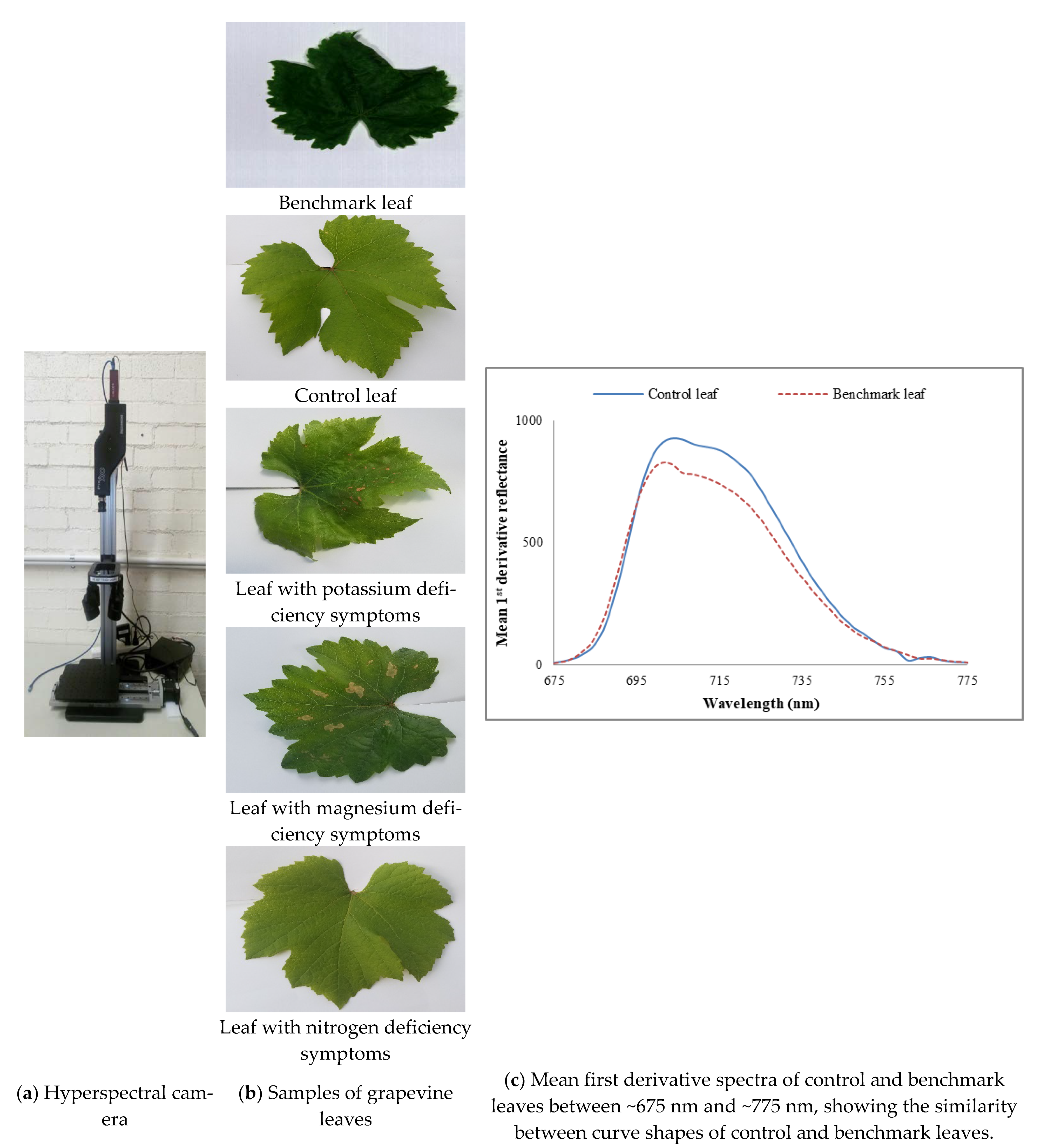
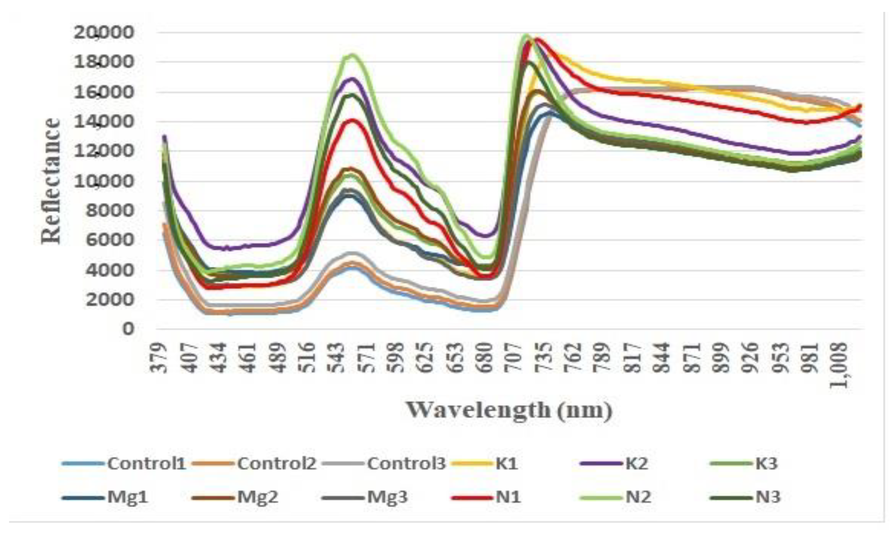
Samples were scanned on the same day of collection to generate HS images by utilising Resonon’s benchtop imaging machine which is presented in Figure 1a. It was comprised of a Pika XC2 HS benchtop camera, mounting tower, linear translation stage, lighting system, and an operating software known as SpectrononPro. The imager and stage were controlled using the SpectrononPro v2.87 software (manufactured by Resonon, Bozeman, MT, USA). This software corrects for dark noise, illumination, and sensor response and provides outputs in standard formats (.bil, .bip, .bsq). It presents spectrum information such as mean spectrum, means first derivatives and means Z profile for scanned samples. Spectral and spatial resolutions of Picka XC2 (i.e., HS imager) were 1.3 nm and 5.86 µm/pixel respectively. The lighting system consisted of four high-intensity halogen lamps that provide stabilised broad-band illumination across the entire measured spectra. Data were collected one line at a time by the imaging spectrometers. This HS imager employed in this study is Resonon’s highest precision device in the ~380–1000 nm wavelength range. An example is shown in Figure 2, where a small portion of each leaf was selected to determine the reflectance across the 380–1000 nm wavelength band. This wavelength range could be divided into three regions: UV: ~380 nm to 400 nm, VIS: ~400+ nm to 700 nm and N.I.R.:~700+ nm to 1000 nm.
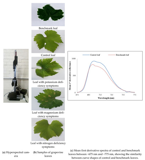
Figure 1.
(a) Hyperspectral camera, (b) samples of grapevine leaves, including the benchmark leaf and (c) mean first derivative spectra of control and benchmark leaves between ~675 nm and ~775 nm, showing the similarity between curve shapes of control and benchmark leaves.

Figure 2.
Reflectance vs. wavelength (nm) for three control, Potassium (K), Magnesium (Mg) and Nitrogen (N) leaves.
The dark current and white reflectance data were collected for calibration. The dark current information was obtained without a light source. White reflectance data were collected by placing a reference material, i.e., a white Teflon sheet of dimension 300 mm × 150 mm × 4 mm on the lighted stage. SpectrononPro subtracts the dark current noise and illumination phenomenon for calibration purposes. Afterward, the system remained calibrated. Sample leaves were then placed on the reference material and scanned for 10000 lines. SpectrononPro produced reflectance of images after removing dark current and white reflectance data from scanned samples. The distance between the leaves and the imager (i.e., the device which records images) was kept at ~57 cm according to the camera manual. The frame rate, integration time, speed unit and scanning speed were set as 62.04 Hz, 244.01 ms, linear and 0.07938 cm/s, respectively, to produce the best HS image quality. Each leaf scan required approximately 5 min to generate an HS image file. They were processed by SpectrononPro software. At first, both sides of the leaves were scanned, but analysis suggested that there was not much difference in characteristics between the upper and lower surfaces of the leaves for the proposed applications. Hence, the results reported here are based on the upper surface of the leaves. It should be mentioned here that we consider the region of interest (ROI) (e.g., a portion from the diseased area) masking in our experiment, then the means are calculated for the spectra of each pixel for each wavelength within the ROI. Subsequently, we consider an average across all the leaves from one group to calculate mean spectra and subsequent features. The data cubes were obtained by selecting the whole area of nutrient-deficient leaves using SpectrononPro v2.87 software.
As nutrient information of these visibly healthy leaves was unknown, to find out a benchmark leaf the mean first derivative reflectance of visibly healthy leaves was compared with that of control leaves. It was found that the mean first derivative reflectance of the tenth leaf from the shoot tip presented the best match to that of the control leaves. Figure 1c reveals that apart from different magnitudes of reflectance, the mean first derivative reflectance of control and benchmark, i.e., the tenth leaves have similar curve shapes indicating the benchmark leaf was a healthy one. Hence, the tenth leaf was chosen as a benchmark leaf.
3. Materials and Methods
At first, we developed nutritional deficiency symptoms in a controlled environment. Then, we captured hyperspectral images and extracted a number of features for our analysis. Those features are normally determined by the average value from a region of leaves in a given spectral band as well as correlation in different bands. Thus, most of the features we used have somehow exploited spectral and spatial dimensions. The rationale of each feature metric, their meaning, and implementations of the values are also provided in the following sub-sections. Section 3.1 describes the development of nutrient deficiency symptoms and benchmark data, Section 3.2 presents the comparison study between visibly healthy and unhealthy leaves, Section 3.3 explains the feature extractions with relevant experimental results and Section 3.4 describes the SVM classification technique.
3.1. Development of Nutrient Deficiency Symptoms and Benchmark Data
This study was undertaken at the National Wine and Grape Industry Centre (NWGIC), Charles Sturt University (CSU), Wagga Wagga, New South Wales (NSW) 2650, Australia. One-year-old dormant cuttings of Vitis vinifera cv. Shiraz were rooted for five weeks and planted in 2.5 L pots containing perlite and established in a glasshouse with 25 °C day and 15 °C night temperatures. The vines were arranged in a randomised block design with eight replicates and fertigated with specific nutrient solutions, where one was a full nutrient treatment (control) based on modified half-strength Hoagland’s solution [40] and the others were the same nutrients, except, potassium (K), magnesium (Mg) and nitrogen (N) were eliminated in K-deficient, Mg-deficient and N-deficient solution, respectively. The contents of calcium (Ca), potassium (K), magnesium (Mg), phosphorus (P), sulphur (S), copper (Cu), iron (Fe), manganese (Mn), molybdenum (Mo) and zinc (Zn) of dried petiole samples collected at the 10-leaf stage from eight replicate plants were assessed by ICP-OES at a commercial diagnostic lab (Charles Sturt University, Wagga Wagga, NSW). Nitrogen was determined on a 50-mg dried and ground sample of the leaf blade with a VarioMAX combustion analyser (Elementar, Hanau, Germany). The K, Mg and N content of the tissues are presented in Table 1. All the other nutrients were in the adequate range and averaged at 3.61% Ca, 0.33% P, 0.17% S, 18 ppm B, 11 ppm Cu, 47 ppm Fe, 85 ppm Mn, 8 ppm Mo and 42 ppm Zn. Images were collected from matured leaves (fully expanded), young leaves separately from Shiraz and Chardonnay for N, K, Mg deficiencies.
The obtained data of both control leaves and nutrient-deficient leaves were then averaged. This study is reported in terms of mean spectral ratio, normalised difference vegetation index (NDVI), mean first derivative reflectance, SD of reflectance and variation index.
3.2. Comparison Study between Visibly Healthy and Unhealthy Leaves
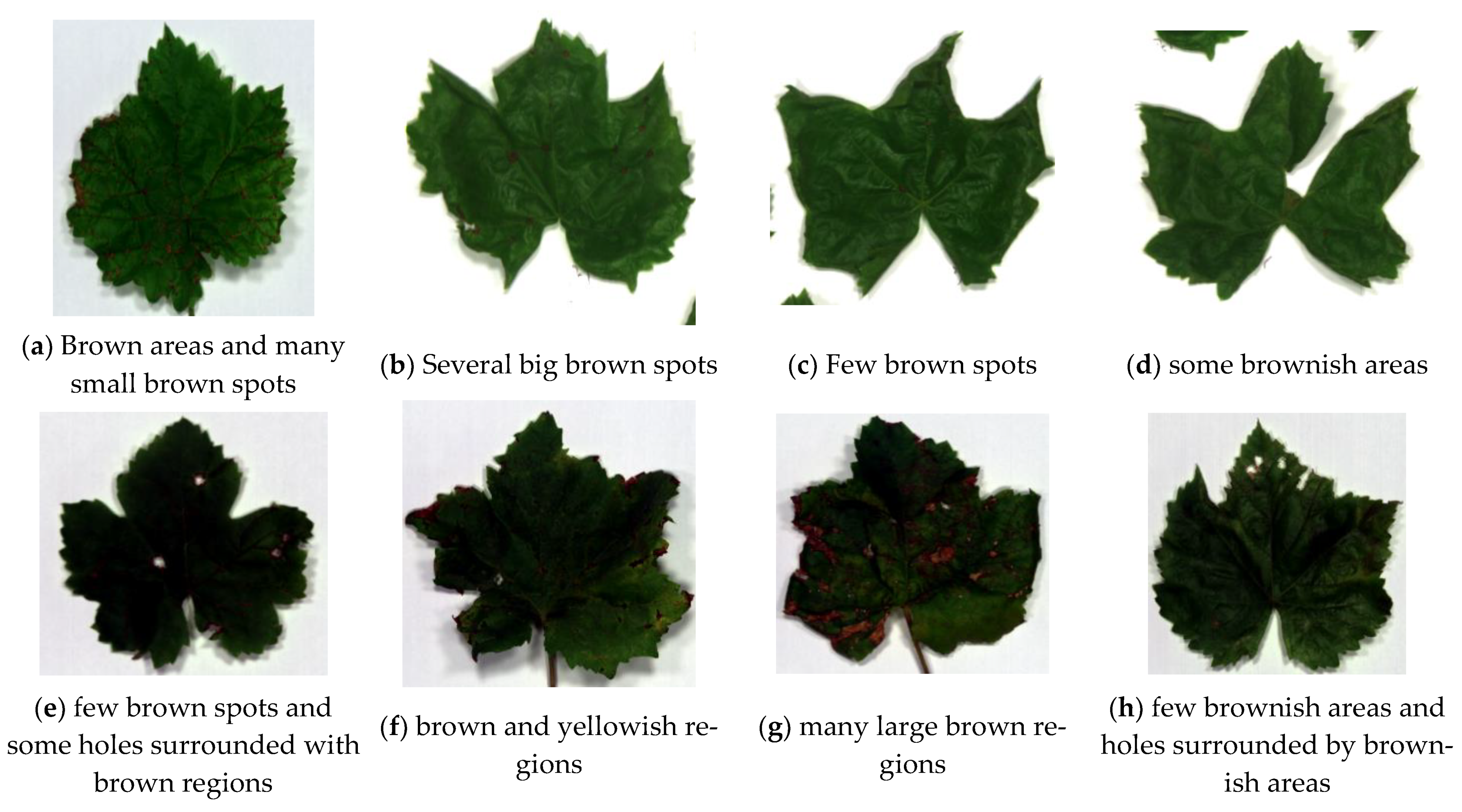
This section presents the comparison study of features for the nine visibly unhealthy leaves with respect to the benchmark leaf (Figure 1b). Figure 3a presents an unhealthy leaf with white spots and a few brown spots. The data cubes were obtained for the whole area and selective areas of leaves to probe the best selection method for distinguishing healthy and unhealthy leaves. Samples of the whole and selective areas’ leaves are presented in Figure 3b,c. The other eight visibly unhealthy samples are shown in Figure 4. The characteristics features of healthy and unhealthy leaves were studied and compared base on mean first derivative reflectance, mean spectral ratios and variation index.
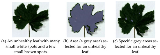
Figure 3.
Unhealthy leaf with white spots and few brown spots and its selected areas for data cube acquisition.

Figure 4.
Sample of unhealthy leaves containing visible defects used for the study of visibly unhealthy leaves.
3.3. Proposed Feature Extractions and Analysis of Physical Features
Two classification schemes were used to assess the captured hyperspectral images. To distinguish healthy from unhealthy leaves a binary classification system was used with the following extracted features: mean first derivative reflectance (Section 3.3.1), mean spectral ratios (Section 3.3.2) and variation index (Section 3.3.3). Using a multiclass classification system, the second set of the extracted features to distinguish individual nutritional deficiencies include: mean the first derivative (Section 3.3.4), mean spectral ratios (Section 3.3.5), normalised difference vegetation index (Section 3.3.6), standard deviation (Section 3.3.7) and variation index (Section 3.3.8).
3.3.1. Mean First Derivative Reflectance for Binary Classification
Mean first derivative of reflectance was considered to distinguish between visibly healthy and unhealthy leaves. It was found that between the ~380 nm and ~675 nm region, other than changes in the magnitude of mean first derivative reflectance, no remarkable information could be obtained for distinguishing between benchmark and the whole area or selective area of unhealthy leaves. Therefore, the first derivative reflectance of healthy and unhealthy leaves between ~380 nm and ~675 nm region are not presented in this manuscript.
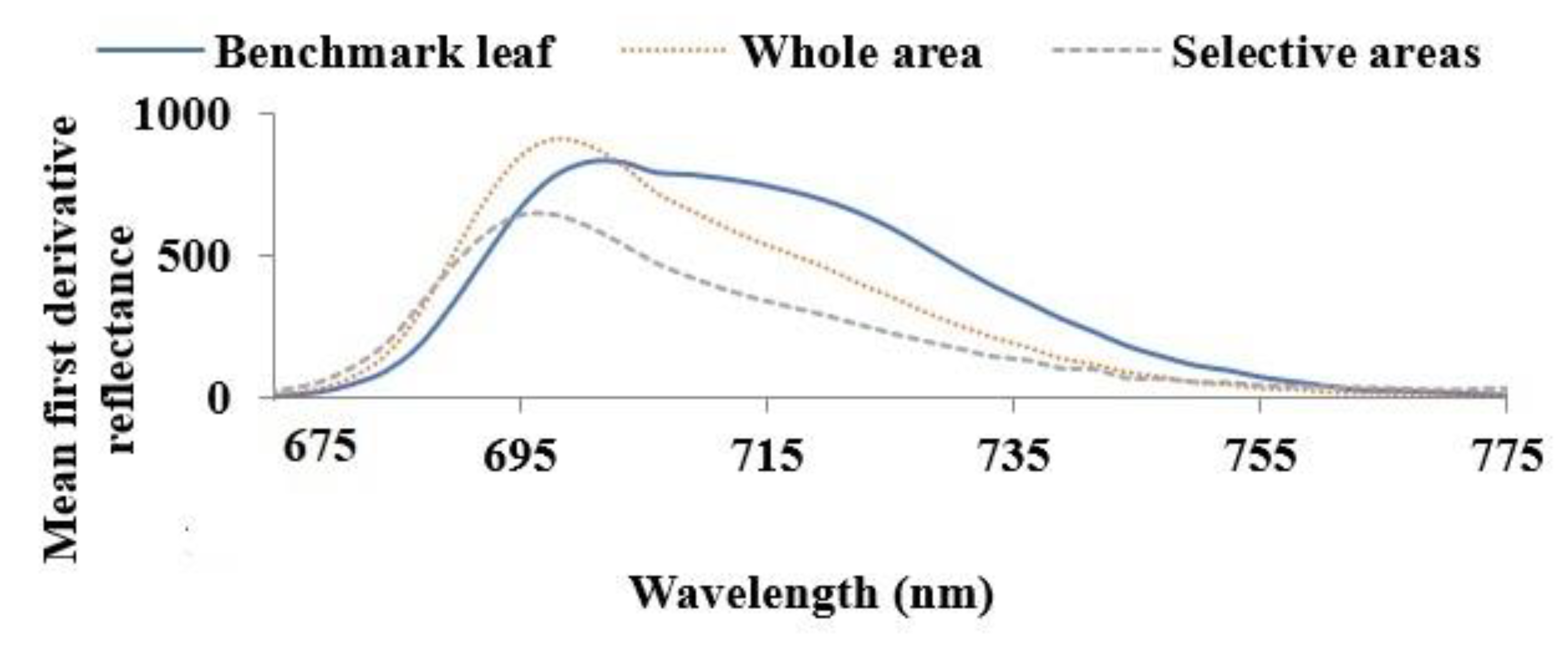
Figure 5 presents the mean first derivative of the reflectance of healthy (benchmark leaf), and unhealthy (whole and selective areas) leaves between ~675 nm to ~775 nm. This figure demonstrates that the mean first derivative reflectance in the N.I.R. wavelength range is higher for unhealthy leaves compared to the benchmark leaf across the entire leaf surface. Narrowing of the reflectance curves for unhealthy leaves is evident for the whole area compared to the benchmark leaf. A shorter wavelength shift of the peak is also observed for unhealthy leaves compared to benchmark leaves. Reflectance is insensitive to changes in chlorophyll content but sensitive to internal leaf structure, water content, structural compounds and altered internal mesophyll structure [41,42] as in the case of the formation of necrotic areas due to tissue decay. Therefore, the deviation of the mean first derivative reflectance curves of unhealthy leaves compared to the benchmark leaf could be due to these differences in internal leaf structures.
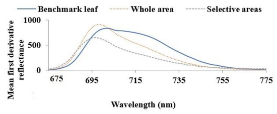
Figure 5.
Mean the first derivative of the reflectance of healthy (benchmark leaf) and unhealthy (whole and selective areas) leaves in the 650 nm to 800 nm range to compare the curve pattern of healthy and unhealthy leaves.
The magnitude of the mean first derivative reflectance for the selective leaf area is lower than the whole leaf surface, though the characteristic curves are similar in appearance. For the case of the selective areas, these were selected based on visible spots or defective regions. Therefore, the characteristic features of only visibly defective areas were obtained. In contrast, for the whole area case, the entire surface of the leaf was selected regardless of visible defects. As a result, the features of both visible and nonvisible defective areas were acquired. Therefore, the selective areas case probes notable features compared to the whole area case and the results of the whole area case are presented afterward.
For most of the unhealthy leaves, similar characteristic curves to Figure 4, such as narrowing and a shift towards shorter wavelengths were observed. It was found that a sharp transition from low to high reflectance usually occurs in the wavelengths between the VIS and N.I.R. regions, and this transition usually shifts to shorter wavelengths in diseased crops [42]. The wavelength where this transition occurs can be observed in the first derivative reflectance curves, as presented in Figure 5. Hence, this deviation of the first derivative reflectance curve shapes could be due to the brown spots in unhealthy leaves. Analysis of the experimental data confirms that the mean first derivative reflectance parameter could distinguish the healthy and most (though not all) unhealthy leaves in the N.I.R. region but not so efficiently in the U.V. and VIS regions.
3.3.2. Mean Spectral Ratios for Binary Classification
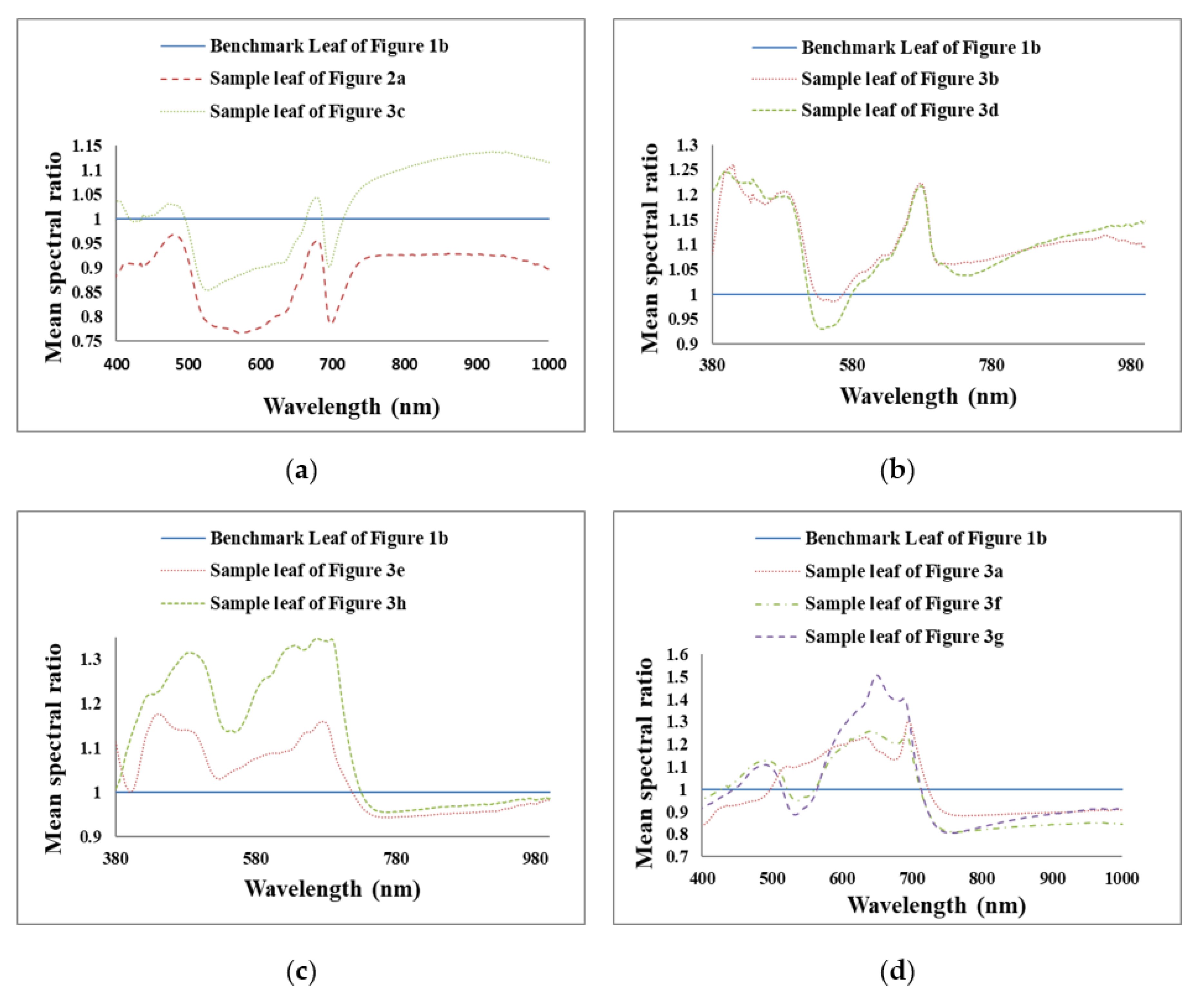
To highlight the comparison between healthy and different unhealthy leaves in all three regions (U.V.: ~380 nm to 400 nm, VIS: ~400+ nm to 700 nm and N.I.R.: ~700+ nm to 1000 nm), the mean reflectance spectra for all the unhealthy leaves were each divided by the mean reflectance spectrum of the representative healthy leaf to obtain mean spectral ratios, i.e., the benchmark leaf (Figure 5) between ~380 nm and 1000 nm. Unhealthy leaves with many small white and few brown spots and unhealthy leaves with few brown spots exhibit almost similar ratio curve trends from ~380 nm to 1000 nm as per Figure 6a. In this figure, the reflectance ratio is higher for unhealthy leaves with few brown spots than that of unhealthy leaves with many small white and few brown spots.
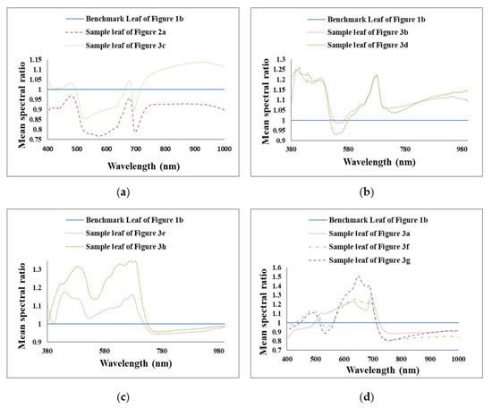
Figure 6.
Mean spectral ratios of different unhealthy leaves (whole area) to benchmark leaf to compare the change in the curve shape of unhealthy leaves with respect to a healthy benchmark leaf. (a) Unhealthy leaves with many small white and few brown spots and unhealthy leaves with few brown spots exhibit almost similar ratio curve trends from ~380 nm to 1000 nm (b) unhealthy leaves with several large brown spots and unhealthy leaves with brownish regions have almost similar ratio curves between the wavelength range 491 nm and 825 nm. (c) the similar shaped ratio curves of unhealthy leaf with brown spots and holes with an unhealthy leaf with brownish regions and holes in the ~400 nm and 1000 nm wavelength range. (d) The unhealthy leaf with brown and yellowish regions and unhealthy leaf with many large brown regions have similar ratio curves with higher ratio values for the latter between ~570 nm to 1000 nm.
From Figure 6b it can be surmised that unhealthy leaves with several large brown spots and unhealthy leaves with brownish regions have almost similar ratio curves. The reflectance ratio of an unhealthy leaf with several large brown spots is more notable than an unhealthy leaf with brownish regions between the wavelength range ~491 nm and ~825 nm. After 825 nm, the reflectance ratio is higher for the unhealthy leaf with brownish regions than the unhealthy leaf with several big brown spots.
Figure 6c compares an unhealthy leaf with brown spots and holes with an unhealthy leaf with brownish regions and holes and shows similarly shaped ratio curves. The reflectance ratio of the former is higher than the latter in the ~400 nm and 1000 nm wavelength range.
From Figure 6d, it can be stated that for whole leaf surface cases, the unhealthy leaf with brown and yellowish regions and unhealthy leaf with many large brown regions have similar ratio curves with higher ratio values for the latter between ~570 nm to 1000 nm. Between ~400 nm and ~570 nm, the ratio value is higher for unhealthy leaves with brown and yellowish regions than that of an unhealthy leaf with many large brown regions. On the other hand, for the unhealthy leaf with brown regions and many small brown spots, the ratio curve is similarly shaped to unhealthy leaves with brown and yellowish regions and unhealthy leaf with many large brown regions between ~603 nm and 1000 nm. From ~400 nm to ~603 nm the unhealthy leaf with brown regions and many small brown spots ratio curves are different from unhealthy leaves with brown and yellowish regions and unhealthy leaf with many large brown regions as well as curves of other unhealthy leaves. Figure 6 indicates that the mean reflectance ratios’ plots could be used to classify different leaf disorders in future work.
3.3.3. Variation Index for Binary Classification
For a further study, a proposed novel parameter, variation index (vi) was defined from the standard deviation (SD) of reflectance as Equation (1):
where vi is the variation index of the ith healthy or unhealthy leaves with respect to the benchmark leaf. σ is the average value of SD of the benchmark leaf and σi is the average value of SDs of the ith healthy or unhealthy leaves.
In the study, the reflectance values obtained for each pixel at each wavelength averaged over the region of interest for each separate wavelength were used. To calculate the variation index, in the N.I.R., the average value of SD was calculated from the reflectance values by selecting the entire N.I.R. (~701 nm to 1000 nm) region for benchmark leaf, four healthy leaves and nine unhealthy leaves individually. Hence, the obtained SD for individual leaves was the averaged value of SD in the N.I.R. region. Then, the average values of SDs of the benchmark and four different healthy leaves were inserted in Equation (1) to obtain the value for variation index for four healthy leaves individually. The same procedure was applied for unhealthy leaves to obtain a variation index of nine unhealthy leaves.
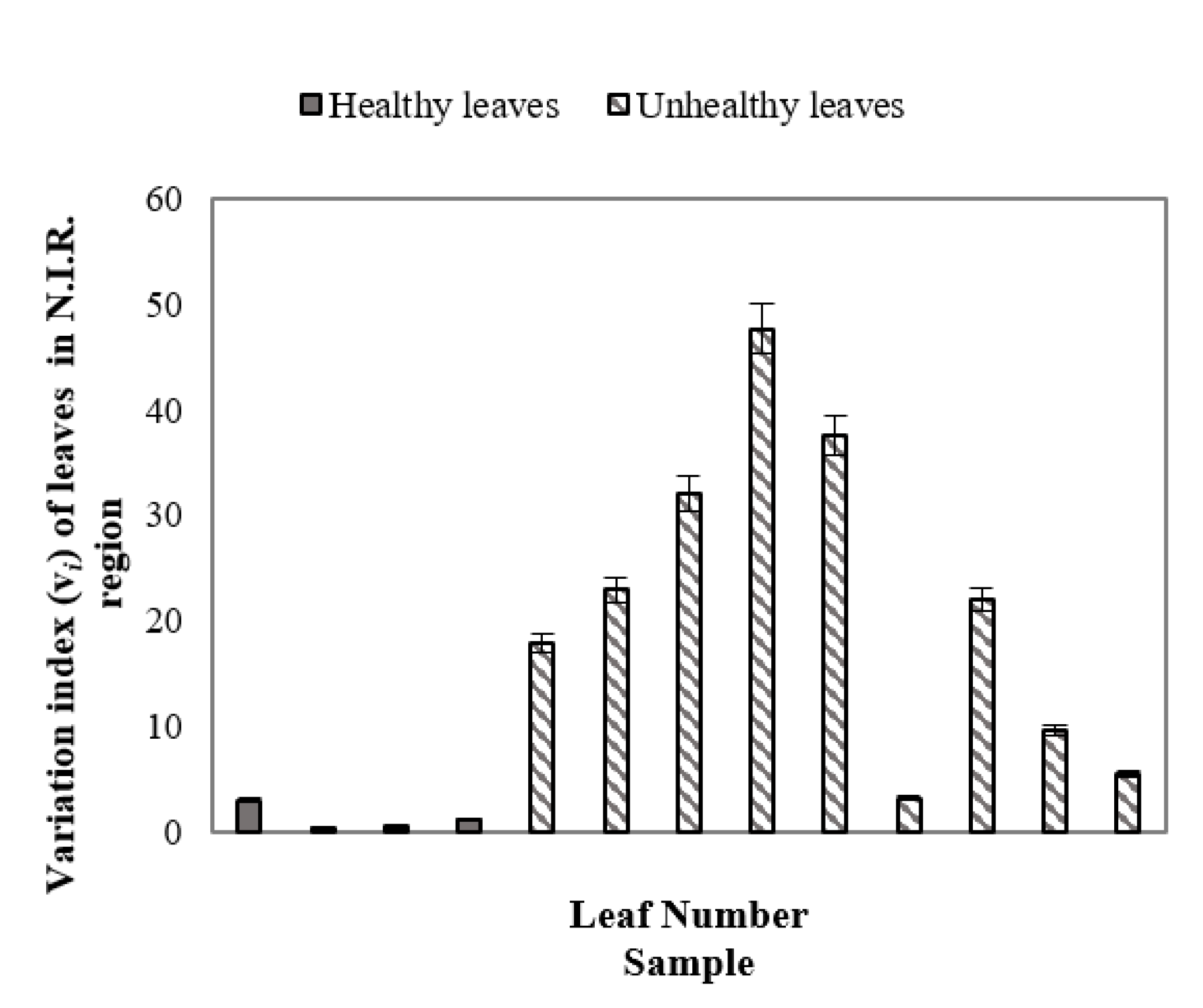
Figure 7 demonstrated the variation index (vi) of healthy and unhealthy leaves in the N.I.R. region (700+ nm to ~1000 nm) where error bars were used to distinguish unhealthy leaves from healthy leaves. As in the previous study, the benchmark leaf was considered as the reference healthy leaf. From Equation (1) it can be stated that the variation index indicates the percentage of the average value of SDs of reflectance of healthy and/or unhealthy leaves differ with respect to the average value of SD of the benchmark leaf. Figure 7 demonstrates that healthy leaves have vi indexes closer to the benchmark leaf, whereas, unhealthy leaves have a higher vi index value at the N.I.R. region, indicating the difference between healthy and unhealthy leaves. Variation indexes for healthy and unhealthy leaves were also calculated using a similar procedure in the UV and VIS regions. However, no such prominent patterns were observed for unhealthy and healthy leaves in the UV and VIS regions (not presented in this manuscript).

Figure 7.
Variation index (vi) of healthy and unhealthy leaves in the N.I.R. region, indicating the difference between healthy and unhealthy leaves.
3.3.4. Mean First Derivative Reflectance for Multiclass Classification
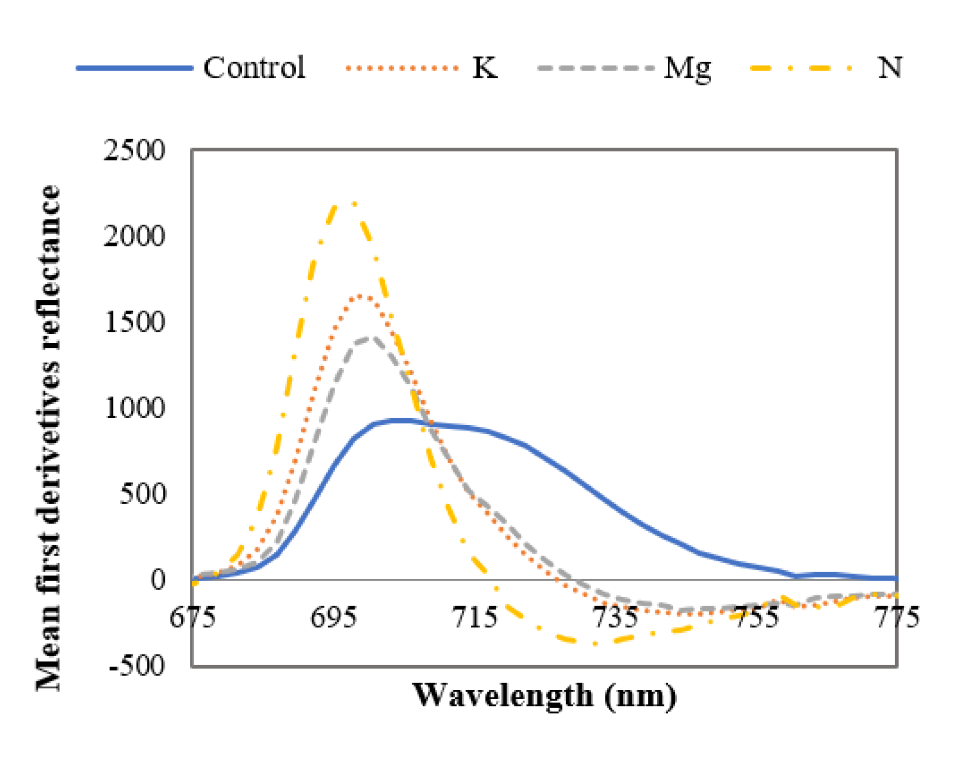
From Figure 8, it can be stated that the ~700 nm derivative peaks are dominant in leaves with nutrient deficiencies, and these results are supported by published findings [43,44]. Narrowing of the first derivative reflectance peak can also be observed for the nutrient-deficient leaves compared to control leaves. The midpoint of this broadened peak is at ~ 708 nm for control leaves. This broadening and narrowing of first derivative peaks for control and nutrient-deficient leaves respectively could be due to the amount of chlorophyll content in the leaves. In this region, the first derivative peak magnitude is ~15%, ~ 9% and 7% higher for N-, K- and Mg-deficient leaves respectively in comparison to control leaves. From Figure 8, it can also be observed that in this wavelength range the first derivative peak of nutrient-deficient leaves has shifted to the shorter wavelength (redshift) compared to the control leaves. It was reported that this shift occurs if vegetation is exposed to low nutrients or environmental stress [43]. No notable curve pattern (broadening or narrowing) of the mean first derivative reflectance was found in the ~380 nm to ~675 nm range to distinguish control and nutrient-deficient leaves.
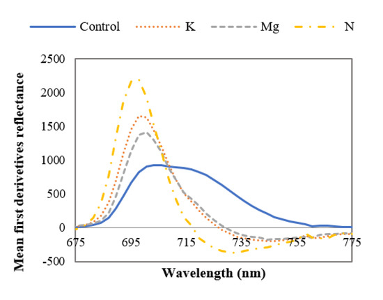
Figure 8.
Mean first derivative spectra of control and nutrient-deficient leaves between ~675 nm and ~775 nm, showing the difference between curve shapes of control and nutrient-deficient leaves.
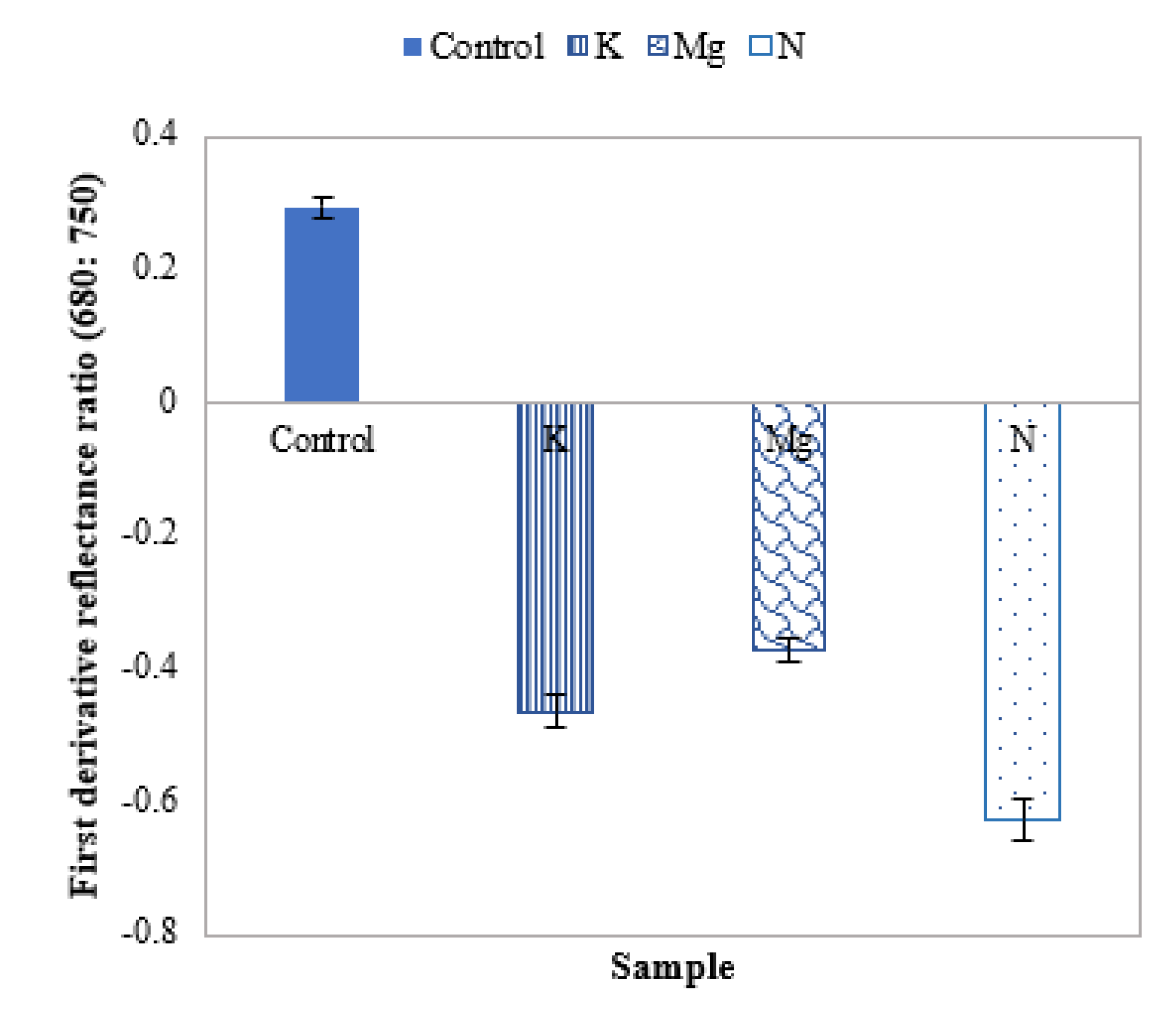
The mean first derivative reflectance shift can further be studied by using the HS derivative ratio in the boundary between the region of the strong absorption of red light by chlorophyll (~680 nm) and the region of high multiple scattering of radiation (~750 nm) [43]. From the first derivative ratio plot of Figure 9, it can be observed that this first derivative ratio is positive for control leaves and negative for nutrient-deficient leaves. Furthermore, the ratio values are ~62%, ~47% and ~37% for N, K and Mg in the negative direction, respectively.

Figure 9.
A plot of the mean first derivative reflectance ratio of control and different nutrient-deficient leaves, representing the difference between control and nutrient-deficient leaves.
3.3.5. Mean Spectral Ratio for Multiclass Classification
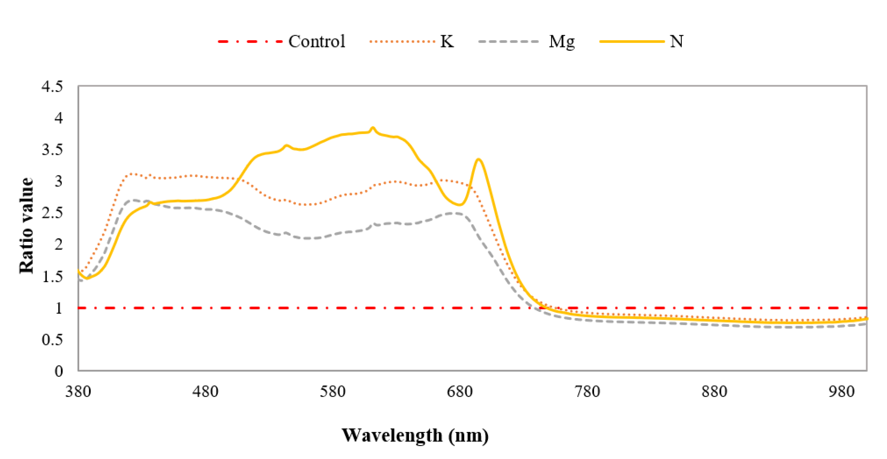
The mean spectral ratio was applied to distinguish features of specific nutrient-deficient leaves with that of control leaves by calculating the reflectance ratios of these different leaf types between 380 nm and 1000 nm. The ratio between the reflectance of nutrient-deficient leaves and that of control leaves is plotted in Figure 10. It can be observed that the shapes of the curves for K- and Mg-deficient leaves are similar, but the magnitude of the spectral ratio of Mg-deficient leaves is lower than that of K-deficient leaves. The curve shape of N-deficient leaves is quite different from those of K -and Mg-deficient leaves. There are peaks between ~650 nm and ~750 nm for N-, Mg- and K-deficient leaves. In this wavelength region peaks at ~693 nm, ~680 nm and ~663 nm were evident for N-, Mg- and K-deficient leaves, respectively. It is also apparent that the magnitude of these peaks at the wavelengths mentioned above is ~3.3, ~2.5 and ~3 times higher for N-, Mg- and K-deficient leaves compared to the control leaves. From the literature it is apparent that many mineral deficiencies cause modifications in the reflectance of leaves compared to the control specimens [45].
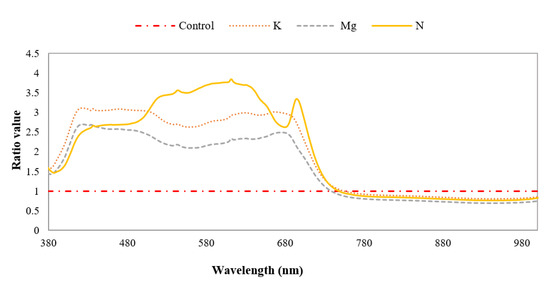
Figure 10.
Mean spectral ratios of different nutrient-deficient leaves to control leaf, distinguishing individually different nutrient-deficient leaves.
3.3.6. Normalised Difference Vegetation Index for Multiclass Classification
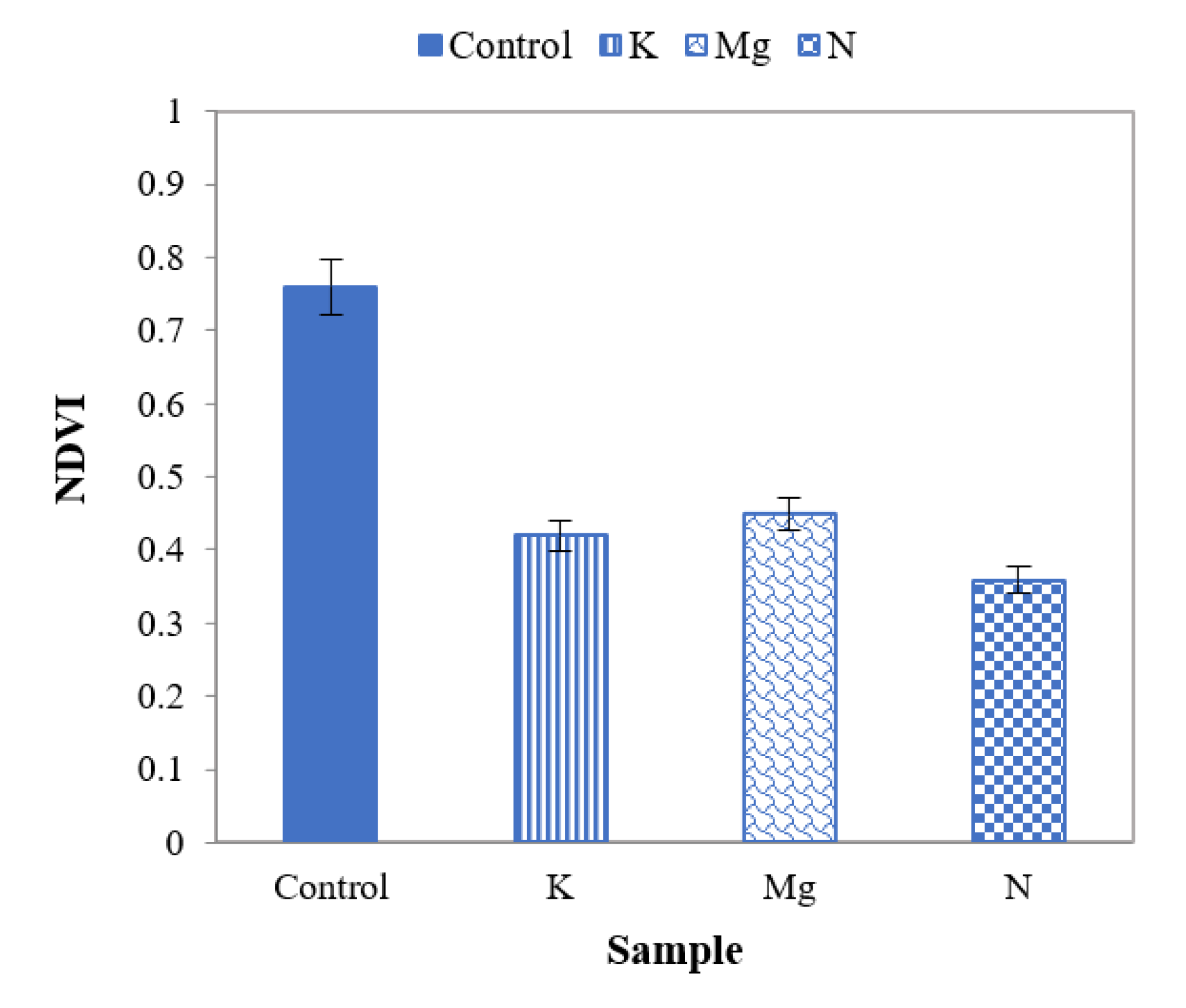
A well-known parameter, the normalised difference vegetation index (NDVI), was applied [41,46] to distinguish features of control and nutrient-deficient leaves. This index describes vegetation by measuring the difference in reflection between near-infrared (which vegetation strongly reflects) and red light (which vegetation absorbs). NDVI always ranges from −1 to +1 where positive values indicate vegetated areas and negative values signify non-vegetated surface features such as water, barren, clouds, and snow. A higher positive value of NDVI refers to healthy and dense vegetation [41]. A number between −1 and 0 suggests an inanimate or dead object, such as roads, buildings, or dead plants. An NDVI plant health rating between 0 and 0.33 indicates unhealthy or stressed plant material, 0.33 to 0.66 is moderately healthy, and 0.66 to 1 is very healthy [46]. It is defined as
The NDVI is calculated for individual images by the following Equation (2), where RED and N.I.R. stand for the spectral reflectance measurements acquired in the RED and near-infrared regions, respectively.
In this NDVI study, an average reflectance value was calculated for the entire RED (~625 nm–~699 nm) range for each control leaf. These averaged values of RED were further averaged to produce a final value for all the control leaves in the RED range to obtain RED reflectance. Similar procedures were followed for the N.I.R. (~701 nm to 1000 nm) region. Applying the same method, the RED and N.I.R. reflectance for K-, Mg-, and N-deficient were calculated.
From NDVI values of Figure 11, it can be observed that they are higher for control leaves than those of nutrient-deficient leaves. These values indicate that control leaves are healthier than leaves with N, K and Mg deficiencies. It is also aparent that the NDVI values for leaves with N, K and Mg deficiencies are not notably different from each other.
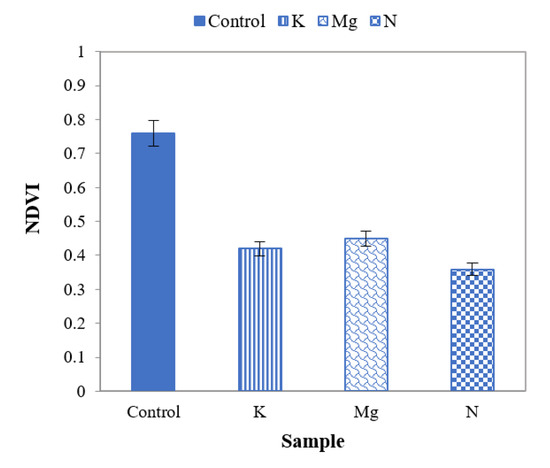
Figure 11.
A plot of NDVI for control and different nutrient-deficient leaves to distinguish control and different nutrient-deficient leaves.
3.3.7. Standard Deviation for Multiclass Classification
The standard deviations (SD) of reflectance were also studied to distinguish features of control and nutrient-deficient leaves (Figure 12). The SDs were calculated for UV (~380 nm to ~400 nm), VIS (+400 nm to ~700 nm) and N.I.R. (+700 nm to 1000 nm) with the average separation of ~2.5 nm between adjacent wavelengths. Figure 12 corroborates that the SD of control leaves in the UV range has the lowest value compared to those of nutrient-deficient leaves. This value is highest for N-deficient leaves with respect to control, K and Mg-deficient leaves. However, the difference of this SD value between K- and Mg-deficient leaves is ~100.
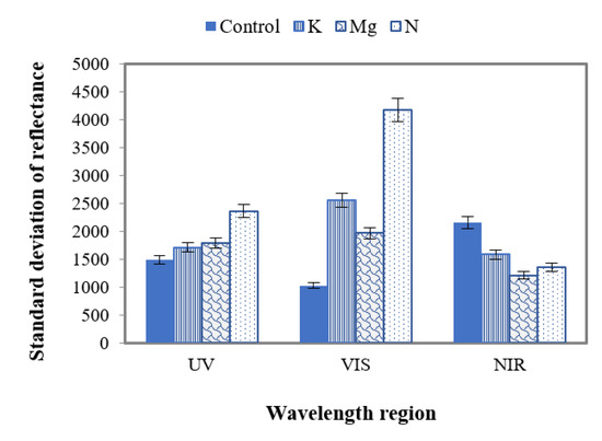
Figure 12.
A plot of SD of control and different nutrient-deficient leaves in UV, VIS and N.I.R. regions, representing the difference between control and nutrient-deficient leaves in different wavelength regions.
In the VIS region (Figure 12), control leaves have the lowest SD value compared to different nutrient-deficient leaves. Here N-deficient leaves have the highest value among these leaves. The difference between SD of K and Mg is 600 in the VIS region. This difference value is higher in the VIS region compared to UV.
In contrast to the UV and VIS regions, in the N.I.R. region the SD value is higher for control leaves than those of nutrient-deficient leaves (Figure 12). In this region, this value was also found to be the lowest for Mg-deficient leaves compared to the K and N counterparts. Here the SD values of N, Mg and K are close to each other. The difference of SD values between N and Mg, N and K, and K and Mg were found to be 100, 300 and 400, respectively.
3.3.8. Variation Index for Multiclass Classification
The variation index vi (Equation (1)) was also applied to distinguish leaves of different nutrient deficiencies individually. This index indicates how much the SDs of the reflectance from nutrient-deficient leaves deviate from the control leaves. In this case, σbenchmark represents the SD of control leaves, and σi represents the SDs of individual nutrient-deficient leaves. Figure 13 presents the variation index of nutrient-deficient leaves with respect to control leaves. The negative value of the variation index (Figure 13) indicates that the values of SDs of nutrient-deficient leaves were higher in the UV (~ 380 nm to 400 nm) and VIS (~400+ nm to 700 nm) regions than that of the control leaf. On the other hand, the positive value of the variation index for nutrient-deficient leaves in the N.I.R. (700+ nm to ~1000 nm) region indicates that the SDs were lower than that of the control leaf.
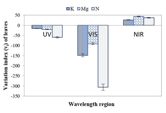
Figure 13.
Variation index (vi) of leaves in the U.V., VIS and N.I.R. regions for distinguishing control and different nutrient-deficient leaves.
From Figure 13, it can be surmised that vi values are ~60%, ~21% and ~16% higher for leaves with N, Mg and K deficiencies respectively in the negative direction in the UV region. This phenomenon indicates that the SD of leaves with a nutrient deficiency is higher than that of the control leaves. In the case of the VIS region (Figure 13), it can be observed that vi values deviate ~31%, ~8% and ~15% for leaves with N, Mg and K deficiencies respectively in the negative direction, indicating that vi of nutrient deficient leaves is higher than that of the control leaves. Furthermore, it can be obtained in Figure 13 that in N.I.R. region vi values deviate ~38%, ~44% and ~27% for leaves with N, Mg and K deficiencies respectively in the positive direction, indicating that here vi of leaves with a nutrient deficiency is lower than that of control leaves. Table 2 presents different essential features and corresponding values for enabling classification to distinguish healthy and nutrient-deficient leaves.

Table 2.
Summary of features for comparison study between control and individual nutrient-deficient leaves.
3.4. SVM Classifier and Performance Evaluation Matrix
An SVM is a supervised machine learning model that uses classification algorithms for two-group classification (i.e., binary) problems. After giving an SVM model a set of labelled training samples for each category, they can categorise new samples. In the first experiment, there were two class classes (i.e., control and unhealthy leaves). For the second experiment, there were four classes (i.e., N, K, Mg disorders and control). Therefore, we customised the SVM in such a way that it can classify binary/multiple classes. The radial basis function kernel (RBF) is usually the first kernel function to be considered. RBF function is used to transformation mapping of samples to a higher-dimensional feature space; therefore, it provides the possibility to solve the nonlinear problem of the samples.
Moreover, the RBF kernel function is only one parameter, while the polynomial kernel function and Sigmoid parameters have more than the RBF kernel function, and this will become more complex in model selection. Therefore, this paper chose the RBF kernel function. Furthermore, we used a cross-validation approach to avoid the bias of the training and testing samples. First, the dataset was shuffled randomly and split it into three groups equally. Then, a group was assigned as testing data and the remaining two groups as training data. Subsequently, the SVM model was fit to the training set and evaluated on the testing set. The evaluation score was retained and the model was discarded. Similar experiments were conducted for each unique group. Then, the performances of the model were summarized.
Each extracted feature, as described in Section 3 and Table 2 (only values), such as the mean first derivative reflectance (wavelength rang 675 nm–775 nm), variation index (700 m–1000 nm) and so on, were considered for training the SVM. Before training the SVM, however, feature scaling was used to bring all values into the [0,1] range to generalise and restrict the range of values. Cross-validation is a common solution when the available datasets are limited [47]. Therefore, to distinguish between a healthy and unhealthy leaf, we considered two healthy leaves and six unhealthy leaves (two leaves from each group) for training the SVM and the remaining four were used for testing. This procedure was repeated three times to implement cross-validation and the performances were noted. A similar procedure was implemented to identify each nutrient deficiency and control leaf for four classes (i.e., Control, K, Mg and N).
To evaluate the overall performances of the proposed technique, we tested evaluation metrics (e.g., precision, recall and F measure). The precision, recall and F measure can be defined by the Equations (3)–(5) [34,48,49]
where Tp (i.e., true positive), Fp (i.e., false positive) and Fn (i.e., false negative) are the values of the actual class (i.e., tissue testing result) as indicated by a specific symptom (or control) and the value of the predicted class is also indicated by the same symptom (or control), the value of the actual class is not indicated by any symptom and the value of the predicted class is indicated by a symptom, the value of actual class not indicated by a specific symptom and the value of the predicted class is not indicated by any symptom. However, either precision or recall alone cannot provide a good indication of a perfect measurement [34]. To be an effective and robust method, it must achieve both high precision and recall. The F measure is defined as combining precision and recall, and is represented by Equation (5).
Matrix Laboratory (MATLAB) 2019b and SpectrononPro (i.e., python language) software were used to perform the experiment. Training the model is very computationally intensive. Therefore, all the experiments are carried out on a dedicated desktop machine DELL OPTIPLEX 9020 (with Intel (R) Xeon (R) E-2124 CPU@ 3.30 GHz (4CPUs), 3.30 GHz 32 GB RAM and 500 GB HDD) running 64-bit Windows 10 operating system.
4. Experimental Results
4.1. Comparison Study between Visibly Healthy and Unhealthy Leaves
Leaf samples were divided into two groups to distinguish between healthy and unhealthy leaves. The first group contained leaves that were visibly unhealthy, and features of these leaves were compared with those of visibly healthy leaves (i.e., benchmark leaf). The variation of curve shapes was highly distinguishable for whole leaf area assessment but less for selective leaf area assessment. Furthermore, the ratio analysis confirmed that for the whole leaf case, comparably more notable curves were apparent. The variation index feature could also identify defective leaves effectively.
4.2. Comparison between Control and Individual Nutrient-Deficient Leaves
The second group of grapevine leaves was incorporated in our analysis to extend our understanding of specific nutrient deficiencies in leaves. These leaves had N, K or Mg deficiencies individually. The features of these leaves were studied relative to those of control leaves and were also compared with each other.
The ratio of the reflectance of nutrient-deficient to control leaves can be used to differentiate N-deficient leaves from K- and Mg-deficient leaves. Furthermore, results suggest that NDVI values could differentiate control and nutrient-deficient leaves, though N, K and Mg deficiencies could not be identified uniquely.
The features of nutrient-deficient leaves between ~650 nm to ~775 nm of first derivative peaks compared to the control leaves could be useful to distinguish between control and nutrient-deficient leaves. Attributes such as a dominant peak at ~700 nm, narrowing of mean first derivative reflectance peaks and first derivative peaks shifted to the shorter wavelength (redshift) are noteworthy.
Mean first derivative reflectance ratio plots between 680 nm and 750 nm could be employed to distinguish control, and nutrient-deficient leaves as this ratio is positive for control leaves and negative for nutrient-deficient leaves. Furthermore, the magnitude of this ratio of different nutrient-deficient leaves could be utilised to identify leaves with N, K and Mg deficiencies.
The study of SD in the UV, VIS and N.I.R. wavelength regions state that this feature could be used to distinguish control and individual nutrient-deficient leaves as different SD values were obtained for N, K and Mg deficiencies.
Additionally, N and K deficiencies could be identified from the variation index analysis in the N.I.R. wavelengths, respectively.
4.3. Experimental Result by Using SVM Algorithm
The performance of the SVM algorithm by using the proposed feature extraction technique is shown in Table 3. This table shows that the precision, recall and F measure is 100% for both the binary and multiclass classification results for the control leaves. For the unhealthy leaves, the F measure performance is 98.14% on average, whereas the overall performance is 98.57% on average. On the other hand, the F measure performance of the multiclass algorithm is 100% for the control and 90.92% nutrient disorder leaves on average. The average F measure is 93.19% which represents the overall performance of the proposed technique. If we can increase the training and testing samples, the performances of the proposed technique may increase.

Table 3.
Performance analasis using the SVM algorithm.
Furthermore, a confusion matrix (Figure 14, (a) binary and (b) multiclass) was used to visualise the performances of the proposed technique. A confusion matrix summary is presented of the number of samples correctly and incorrectly identified and separated into each class with a number, where the diagonal and off-diagonal elements represent correctly and incorrectly identified samples respectively. It should be mentioned here that we are presenting only one group of experimental results and the average result of three iterations is shown in Table 3.
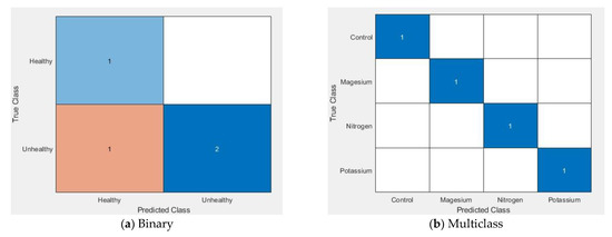
Figure 14.
Confusion matrix for the binary and multiclass classifier.
5. Conclusions and Future Work
This paper presents an experimental comparative study of healthy and unhealthy grapevine leaves and individual nutrient-deficient leaves utilising an HS camera in the UV, VIS and N.I.R. wavelength ranges (~380 nm to 1000 nm). It suggests that this technology could be efficiently employed to obtain reliable results in this domain. Features such as reflectance ratio, mean first derivative reflectance, variation index, mean spectral ratio, normalised difference vegetation index (NDVI) and standard deviation (SD) were applied in this study.
From the analysis it was found the mean first derivative reflectance curve shape between ~675 nm and ~775 nm and the variation index in the N.I.R. region can differentiate healthy from unhealthy leaves. In contrast, mean spectral ratios can be used as a tool to classify the individual nutritional disorders.
Features such as NDVI, mean first derivative reflectance from ~675 to ~775 nm, and SD in the N.I.R. region can also be applied as features to distinguish between control and nutrient-deficient leaves. The ratio reflectance between control and nutrient-deficient leaves can be used to identify an individual nutrient deficiency. Moreover, the variation index in the N.I.R. region can be a feature to distinguish K deficiency from N and Mg deficiencies. Control and an individual nutrient deficiency can be identified with the aid of SD in the VIS region and first derivative reflectance ratio (680 nm: 750 nm). To identify N-deficiency, SD in the UV region can be applied. If required, a vineyard-specific database of control leaves may be created following confirmation with chemical tissue analysis. However, ideally, this step will not be required if regional and cultivar-specific databases are assembled and made freely accessible.
In the future we envisage analysing all or most of the micro and macronutrients that grapevines require including but not limited to:
Micro-nutrients: copper (Cu), iron (Fe), manganese (Mn), boron (B), chlorine (Cl);
Macro-nutrients: calcium (Ca), oxygen (O), sulphur (S), phosphorus (P), carbon (C).
The results presented here are based on leaves obtained from glasshouse plants grown under controlled conditions. Further field-based trials using vines grown under diverse environmental stresses are required to extend these findings to practical scenarios. This will allow the implementation of new viticultural management strategies that are not only based on chemical tissue analyses but also HSI so that the appropriate fertilisers and soil amendments can be applied in a timely fashion. A hand-held, tractor mounted or airborne tool with the capability of a highly accurate diagnosis, even prior to visual symptom appearance, will be ideal for timely treatment. This can be achieved on a single vine basis through HSI so that localized treatments can be applied. This precision will reduce the overall quantity of agrichemicals required and thus will lead to more sustainable vineyard management and environmental protection. Repeated plant tissue assessments over the course of the season will also mean that corrective action can be taken rapidly so that yield and quality losses are curtailed or even prevented. With advances in the processing and analyzing of hyperspectral imagery, this technique can eventually be extended to practical applications that are flexible and cost-effective.
Author Contributions
Methodology, S.D.; formal analysis, validation, M.P., L.Z. T.D. and D.M.M.R.; investigation, S.Y.R.; data curation, T.B.; writing—original draft preparation, S.D. and D.M.M.R.; writing—review and editing, M.P. and S.Y.R.; visualization, D.M.M.R.; supervision, M.P., T.D. and L.Z.; funding acquisition, S.Y.R. and L.M.S. All authors have read and agreed to the published version of the manuscript.
Funding
This research was funded by Wine Australia, grant number CSU 1702-3.
Conflicts of Interest
The authors declare no conflict of interest.
References
- Kishore, M.; Kulkarni, S.B. Hyperspectral imaging technique for plant leaf identification. In Proceedings of the 2015 International Conference on Emerging Research in Electronics, Computer Science and Technology ICERECT 2015, Mandya, India, 17–19 December 2015; pp. 209–213. [Google Scholar] [CrossRef]
- Ariana, D.P.; Lu, R. Hyperspectral waveband selection for internal defect detection of pickling cucumbers and whole pickles. Comput. Electron. Agric. 2010, 74, 137–144. [Google Scholar] [CrossRef]
- Rajkumar, P.; Wang, N.; Eimasry, G.; Raghavan, G.; Gariepy, Y. Studies on banana fruit quality and maturity stages using hyperspectral imaging. J. Food Eng. 2012, 108, 194–200. [Google Scholar] [CrossRef]
- Zhang, C.; Guo, C.; Liu, F.; Kong, W.; He, Y.; Lou, B. Hyperspectral imaging analysis for ripeness evaluation of strawberry with support vector machine. J. Food Eng. 2016, 179, 11–18. [Google Scholar] [CrossRef]
- Sun, M.; Zhang, D.; Liu, L.; Wang, Z. How to predict the sugariness and hardness of melons: A near-infrared hyperspectral imaging method. Food Chem. 2017, 218, 413–421. [Google Scholar] [CrossRef]
- Susič, N.; Žibrat, U.; Širca, S.; Strajnar, P.; Razinger, J.; Knapič, M.; Vončina, A.; Urek, G.; Stare, B.G. Discrimination between abiotic and biotic drought stress in tomatoes using hyperspectral imaging. Sens. Actuators B Chem. 2018, 273, 842–852. [Google Scholar] [CrossRef] [Green Version]
- Ge, Y.; Bai, G.; Stoerger, V.; Schnable, J. Temporal dynamics of maize plant growth, water use, and leaf water content using automated high throughput RGB and hyperspectral imaging. Comput. Electron. Agric. 2016, 127, 625–632. [Google Scholar] [CrossRef] [Green Version]
- Pandey, P.; Ge, Y.; Stoerger, V.; Schnable, J.C. High Throughput In vivo Analysis of Plant Leaf Chemical Properties Using Hyperspectral Imaging. Front. Plant Sci. 2017, 8, 1348. [Google Scholar] [CrossRef] [PubMed] [Green Version]
- Tung, K.-C.; Tsai, C.-Y.; Hsu, H.-C.; Chang, Y.-H.; Chang, C.-H.; Chen, S. Evaluation of Water Potentials of Leafy Vegetables Using Hyperspectral Imaging. IFAC-Pap. 2018, 51, 5–9. [Google Scholar] [CrossRef]
- Moghadam, P.; Ward, D.; Goan, E.; Jayawardena, S.; Sikka, P.; Hernandez, E. Plant disease detection using hyperspectral imaging. In Proceedings of the International Conference on Digital Image Computing: Techniques and Applications, Sydney, NSW, Australia, 29 November–1 December 2017; pp. 1–8. [Google Scholar] [CrossRef]
- Lowe, A.; Harrison, N.; French, A.P. Hyperspectral image analysis techniques for the detection and classification of the early onset of plant disease and stress. Plant Methods 2017, 13, 80. [Google Scholar] [CrossRef]
- Lee, W.-H.; Kim, M.S.; Lee, H.; Delwiche, S.R.; Bae, H.; Kim, D.-Y.; Cho, B.-K. Hyperspectral near-infrared imaging for the detection of physical damages of pear. J. Food Eng. 2014, 130, 1–7. [Google Scholar] [CrossRef]
- Zhang, N.; Liu, X.; Jin, X.; Li, C.; Wu, X.; Yang, S.; Ning, J.; Yanne, P. Determination of total iron-reactive phenolics, anthocyanins and tannins in wine grapes of skins and seeds based on near-infrared hyperspectral imaging. Food Chem. 2017, 237, 811–817. [Google Scholar] [CrossRef]
- Baca-Bocanegra, B.; Nogales-Bueno, J.; Hernández-Hierro, J.M.; Heredia, F.J. Evaluation of extractable polyphenols released to wine from cooperage byproduct by near infrared hyperspectral imaging. Food Chem. 2018, 244, 206–212. [Google Scholar] [CrossRef]
- Gomes, V.M.; Fernandes, A.M.; Faia, A.; Melo-Pinto, P. Comparison of different approaches for the prediction of sugar content in new vintages of whole Port wine grape berries using hyperspectral imaging. Comput. Electron. Agric. 2017, 140, 244–254. [Google Scholar] [CrossRef]
- Gutiérrez, S.; Novales, J.F.; Diago, M.P.; Tardaguila, J. On-The-Go Hyperspectral Imaging Under Field Conditions and Machine Learning for the Classification of Grapevine Varieties. Front. Plant Sci. 2018, 9, 1102. [Google Scholar] [CrossRef]
- Loggenberg, K.; Strever, A.; Greyling, B.; Poona, N. Modelling Water Stress in a Shiraz Vineyard Using Hyperspectral Imaging and Machine Learning. Remote. Sens. 2018, 10, 202. [Google Scholar] [CrossRef] [Green Version]
- Bendel, N.; Kicherer, A.; Backhaus, A.; Köckerling, J.; Maixner, M.; Bleser, E.; Klück, H.-C.; Seiffert, U.; Voegele, R.T.; Töpfer, R. Detection of Grapevine Leafroll-Associated Virus 1 and 3 in White and Red Grapevine Cultivars Using Hyperspectral Imaging. Remote. Sens. 2020, 12, 1693. [Google Scholar] [CrossRef]
- Mehrubeoglu, M.; Orlebeck, K.; Zemlan, M.J.; Autran, W. Detecting red blotch disease in grape leaves using hyperspectral imaging. Algorithms Technol. Multispectral Hyperspectral Ultraspectral Imag. XXII 2016, 9840, 98400. [Google Scholar] [CrossRef]
- Retallack, M. GRAPEVINE BIOLOGY. Available online: http://www.viti.com.au/pdf/MVWGG%20Fact%20Sheet—Grapevine%20Biology.pdf (accessed on 9 March 2021).
- Hopper, D.W.; Ghan, R.; Cramer, G.R. A rapid dehydration leaf assay reveals stomatal response differences in grapevine genotypes. Hortic. Res. 2014, 1, 2. [Google Scholar] [CrossRef] [PubMed] [Green Version]
- Fisher, D.; Wicks, T. Powdery Mildew in Wine Grapes in Western Australia. 2003. Available online: https://researchlibrary.agric.wa.gov.au/bulletins (accessed on 9 March 2021).
- Knauer, U.; Matros, A.; Petrovic, T.; Zanker, T.; Scott, E.S.; Seiffert, U. Improved classification accuracy of powdery mildew infection levels of wine grapes by spatial-spectral analysis of hyperspectral images. Plant Methods 2017, 13, 1–15. [Google Scholar] [CrossRef] [PubMed]
- Proffitt, T.; Campbell-Clause, J. Managing Grapevine Nutrition and Vineyard Soil Health Perth Region NRM. 2012. Available online: www.winewa.asn.au (accessed on 9 March 2021).
- Thomidis, T.; Zioziou, E.; Koundouras, S.; Karagiannidis, C.; Navrozidis, I.; Nikolaou, N. Effects of nitrogen and irrigation on the quality of grapes and the susceptibility to Botrytis bunch rot. Sci. Hortic. 2016, 212, 60–68. [Google Scholar] [CrossRef]
- Zlámalová, T.; Elbl, J.; Baron, M.; Bělíková, H.; Lampíř, L.; Hlušek, J.; Lošák, T. Using foliar applications of magnesium and potassium to improve yields and some qualitative parameters of vine grapes (Vitis vinifera L.). Plant Soil Environ. 2016, 61, 451–457. [Google Scholar] [CrossRef] [Green Version]
- Martín, P.; Zarco-Tejada, P.J.; González, M.R.; Berjón, A. Using hyperspectral remote sensing to map grape quality in ‘Tempranillo’ vineyards affected by iron deficiency chlorosis. J. Grapevine Res. 2007, 46, 7–14. [Google Scholar] [CrossRef]
- Debnath, T.; Debnath, S.; Paul, M. Detection of Age and Defect of Grapevine Leaves Using Hyper Spectral Imaging. In Transactions on Petri Nets and Other Models of Concurrency XV; Springer Science and Business Media: Berlin, Germany, 2019; pp. 92–105. [Google Scholar]
- Zhang, X.; Qiao, Y.; Meng, F.; Fan, C.; Zhang, M. Identification of Maize Leaf Diseases Using Improved Deep Convolutional Neural Networks. IEEE Access 2018, 6, 30370–30377. [Google Scholar] [CrossRef]
- Hlaing, C.S.; Zaw, S.M.M. Model-based statistical features for mobile phone image of tomato plant disease classification. Parallel Distrib. Comput. Appl. Technol. PDCAT Proc. 2018, 2017, 223–229. [Google Scholar] [CrossRef]
- Bin Husin, Z.; Shakaff, A.Y.B.M.; Aziz, A.H.B.A.; Farook, R.B.S.M. Feasibility Study on Plant Chili Disease Detection Using Image Processing Techniques. In Proceedings of the Third International Conference on Intelligent Systems Modelling and Simulation, Kota, Kinabalu, 8–10 February 2012; pp. 291–296. [Google Scholar] [CrossRef]
- Islam, M.; Anh, D.; Wahid, K.; Bhowmik, P. Detection of potato diseases using image segmentation and multiclass support vector machine. In Proceedings of the 2017 IEEE 30th Canadian Conference on Electrical and Computer Engineering (CCECE), Windsor, ON, Canada, 30 April–3 May 2017; pp. 1–4. [Google Scholar]
- Huang, W.; Guan, Q.; Luo, J.; Zhang, J.; Zhao, J.; Liang, D.; Huang, L.; Zhang, D. New Optimized Spectral Indices for Identifying and Monitoring Winter Wheat Diseases. IEEE J. Sel. Top. Appl. Earth Obs. Remote. Sens. 2014, 7, 2516–2524. [Google Scholar] [CrossRef]
- Rahaman, D.M.M.; Baby, T.; Oczkowski, A.; Paul, M.; Zheng, L.; Schmidtke, L.; Holzapfel, B.P.; Walker, R.R.; Rogiers, S.Y. Grapevine Nutritional Disorder Detection Using Image Processing. In Transactions on Petri Nets and Other Models of Concurrency XV; Springer Science and Business Media: Berlin, Germany, 2019; pp. 184–196. [Google Scholar]
- Phadikar, S.; Sil, J. Rice disease identification using pattern recognition techniques. In Proceedings of the 11th International Conference on Computer and Information Technology, Khulna, Bangladesh, 24–27 December 2008; pp. 420–423. [Google Scholar] [CrossRef]
- Ren, T.; Zhang, Y.; Wang, C. Identification of Corn Leaf Disease Based on Image Processing. In Proceedings of the 2nd International Conference on Information Systems and Computer Aided Education ICISCAE 2019, Dalian, China, 28–30 September 2019; pp. 165–168. [Google Scholar] [CrossRef]
- Li, C.; Lanying, W. Research on Application of Probability Neural Network in Maize Leaf Disease Identification. J. Agric. Mech. Researc 2011, 6. Available online: http://en.cnki.com.cn/Article_en/CJFDTOTAL-NJYJ201106040.htm (accessed on 22 July 2020).
- Liangfeng, X.; Xiaobing, X.; Min, H.; Rujing, W.; Chengjun, X.; Hongbo, C. Corn leaf disease identification based on multiple classifiers fusion. Trans. Chin. Soc. Agric. Eng. 2015, 31, 194–201. Available online: https://www.ingentaconnect.com/content/tcsae/tcsae/2015/00000031/00000014/art00027# (accessed on 22 July 2020).
- Alehegn, E. Maize Leaf Diseases Recognition and Classification Based on Imaging and Machine Learning Techniques. Int. J. Innov. Res. Comput. Commun. Eng. 2017, 5, 1–11. [Google Scholar]
- Baby, T.; Hocking, B.; Tyerman, S.; Gilliham, M.; Collins, C. Modified Method for Producing Grapevine Plants in Controlled Environments. Am. J. Enol. Vitic. 2014, 65, 261–267. [Google Scholar] [CrossRef]
- Neuwirthová, E.; Lhotáková, Z.; Albrechtova, J. The Effect of Leaf Stacking on Leaf Reflectance and Vegetation Indices Measured by Contact Probe during the Season. Sensors 2017, 17, 1202. [Google Scholar] [CrossRef] [Green Version]
- Gazala, I.F.S.; Sahoo, R.N.; Pandey, R.; Mandal, B.; Gupta, V.K.; Singh, R.; Sinha, P. Spectral reflectance pattern in soybean for assessing yellow mosaic disease. Indian J. Virol. 2013, 24, 242–249. [Google Scholar] [CrossRef] [Green Version]
- Siciliano, D.; Wasson, K.; Potts, D.C.; Olsen, R. Evaluating hyperspectral imaging of wetland vegetation as a tool for detecting estuarine nutrient enrichment. Remote. Sens. Environ. 2008, 112, 4020–4033. [Google Scholar] [CrossRef] [Green Version]
- Mutanga, O.; Skidmore, A. Red edge shift and biochemical content in grass canopies. ISPRS J. Photogramm. Remote. Sens. 2007, 62, 34–42. [Google Scholar] [CrossRef]
- Rustioni, L.; Grossi, D.; Brancadoro, L.; Failla, O. Iron, magnesium, nitrogen and potassium deficiency symptom discrimination by reflectance spectroscopy in grapevine leaves. Sci. Hortic. 2018, 241, 152–159. [Google Scholar] [CrossRef]
- NDVI and Your Farm: Understanding NDVI for Plant Health. Available online: https://www.agriculture-xprt.com/news/ndvi-and-your-farm-understanding-ndvi-for-plant-health-insights-702065 (accessed on 7 August 2021).
- Vabalas, A.; Gowen, E.; Poliakoff, E.; Casson, A.J. Machine learning algorithm validation with a limited sample size. PLoS ONE 2019, 14, e0224365. [Google Scholar] [CrossRef] [PubMed]
- Shoumy, N.J.; Ang, L.; Rahaman, D.M.M. Multimodal Information Processing and Big Data Analytics in a Digital World. In Multimodal Analytics for Next-Generation Big Data Technologies and Applications; Seng, K., Ang, L., Liew, A.C., Gao, J., Eds.; Springer Nature Switzerland AG: Basingstoke, UK, 2019; pp. 45–71. [Google Scholar]
- Paul, M.; Salehin, M. Spatial and Motion Saliency Prediction Method Using Eye Tracker Data for Video Summarization. IEEE Trans. Circuits Syst. Video Technol. 2018, 29, 1856–1867. [Google Scholar] [CrossRef]
Publisher’s Note: MDPI stays neutral with regard to jurisdictional claims in published maps and institutional affiliations. |
© 2021 by the authors. Licensee MDPI, Basel, Switzerland. This article is an open access article distributed under the terms and conditions of the Creative Commons Attribution (CC BY) license (https://creativecommons.org/licenses/by/4.0/).

