Figure 1.
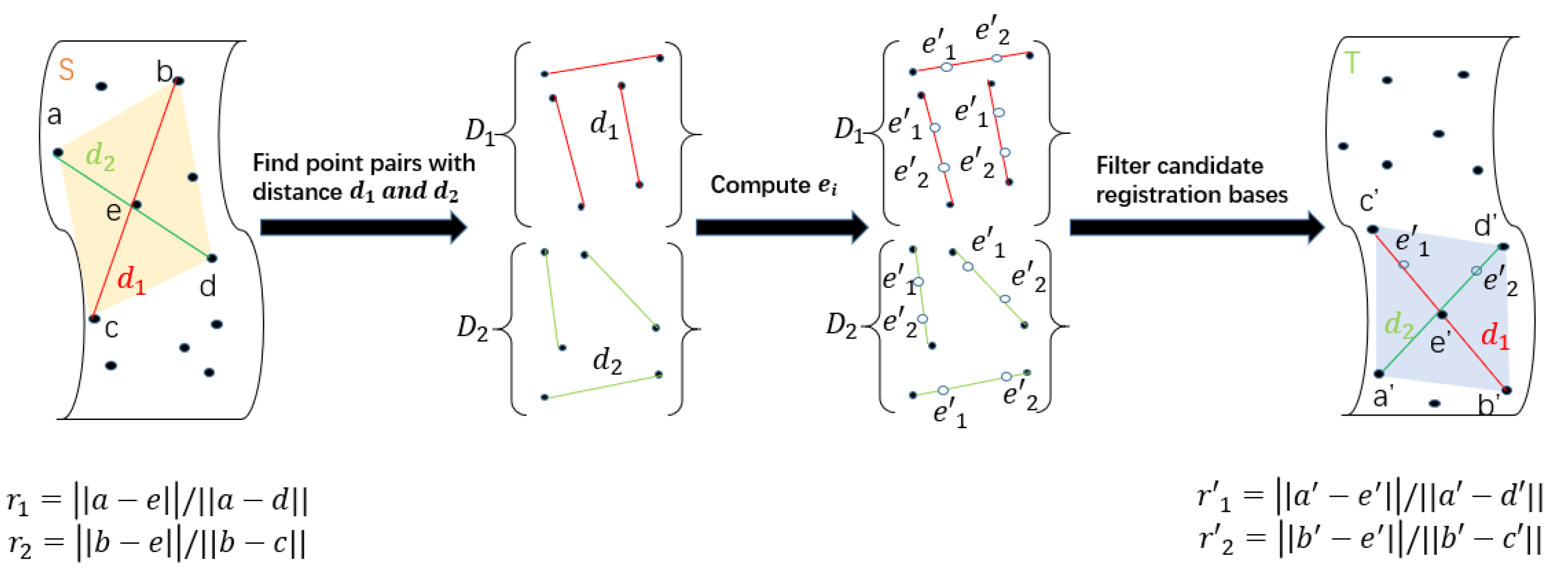
The flowchart of 4PCS. Given the registration base composed of four coplanar points a, b, c, and d in source point cloud S, calculate the intersection point e, affine invariants , and the distance and between diagonal points. Then point pairs extracting in target point cloud T and the intersection points calculating according to are performed in turn where and are point pair sets with distance and among point pairs, respectively. Finally, construct the target registration base pair according to the intersection point .
Figure 1.
The flowchart of 4PCS. Given the registration base composed of four coplanar points a, b, c, and d in source point cloud S, calculate the intersection point e, affine invariants , and the distance and between diagonal points. Then point pairs extracting in target point cloud T and the intersection points calculating according to are performed in turn where and are point pair sets with distance and among point pairs, respectively. Finally, construct the target registration base pair according to the intersection point .
Figure 2.
The flowchart of the Super Edge 4PCS. The original point clouds are taken as the inputs. After boundary segmentation, overlapping regions extraction, corresponding bases acquisition, we can obtain registration base pair set including base and . The transformation matrix is estimated from , then the final transformed point cloud is outputed.
Figure 3.
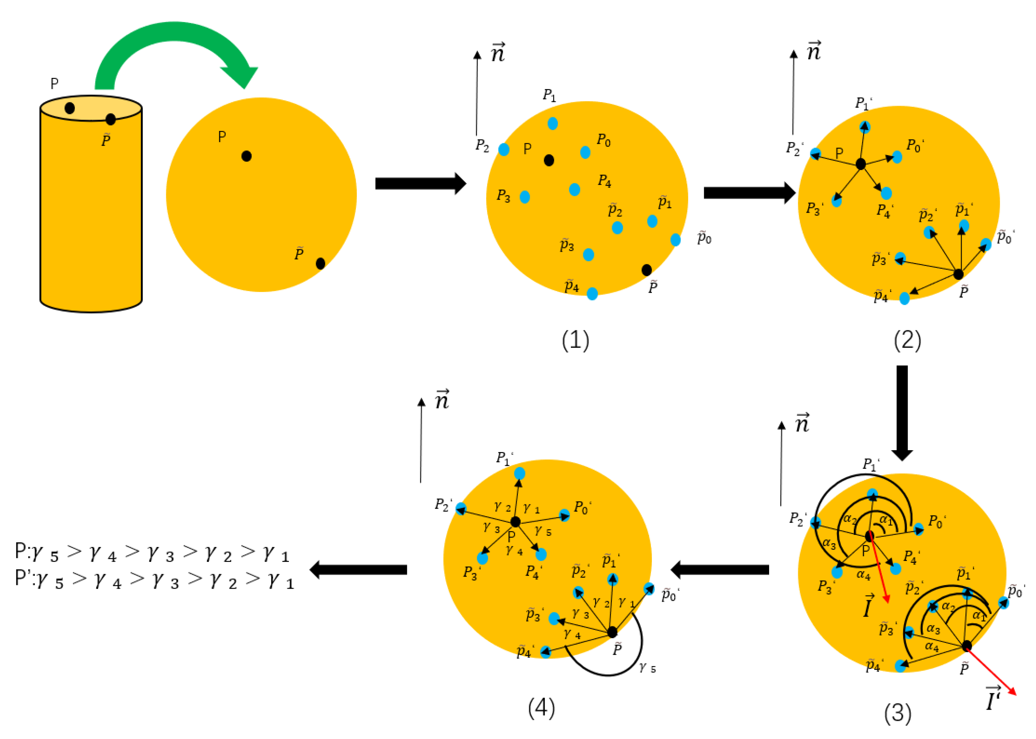
The flowchart of boundary segmentation. P and are interest points, , are neighbor points of interest points P and , respectively. and are the mapping points of , on the tangent plane of point P. is the normal vector of the tangent plane . are the angles between the vectors and , and are the angles between two adjacent mapping vectors.
Figure 3.
The flowchart of boundary segmentation. P and are interest points, , are neighbor points of interest points P and , respectively. and are the mapping points of , on the tangent plane of point P. is the normal vector of the tangent plane . are the angles between the vectors and , and are the angles between two adjacent mapping vectors.
Figure 4.
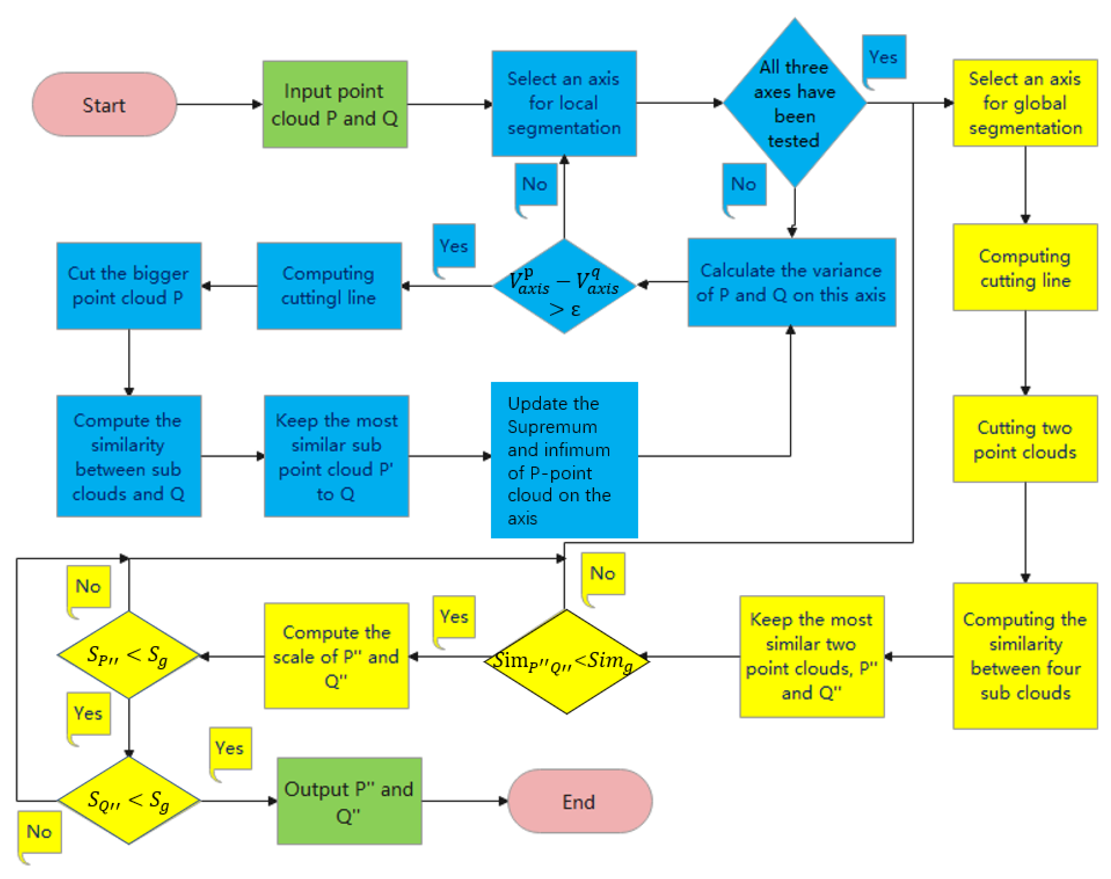
Overlapping regions extraction. Blue part represents local segmentation, yellow part represents global segmentation and green part represents the input ans output of the method. It finally outputs two divided sub point clouds as the overlapping regions. and represent the variance of P point cloud and Q point cloud on three coordinate axis; represents the similarity of the overlapping regions and ; represents the similarity threshold for stopping segmentation; and represent the scale of overlapping regions and ; represents the scale threshold to stop segmentation.
Figure 4.
Overlapping regions extraction. Blue part represents local segmentation, yellow part represents global segmentation and green part represents the input ans output of the method. It finally outputs two divided sub point clouds as the overlapping regions. and represent the variance of P point cloud and Q point cloud on three coordinate axis; represents the similarity of the overlapping regions and ; represents the similarity threshold for stopping segmentation; and represent the scale of overlapping regions and ; represents the scale threshold to stop segmentation.
Figure 5.
Local overlapping regions extraction of the larger point cloud. This figure employs two-dimensional object segmentation as an example to show the process of local overlapping regions extraction. The three-dimensional situation can be derived accordingly. The cutting line approach the ground-truth segmentation axis by updating the supremum and infimum of cutting direction where and represent the upper and lower bounds of the point cloud S on the x-axis.
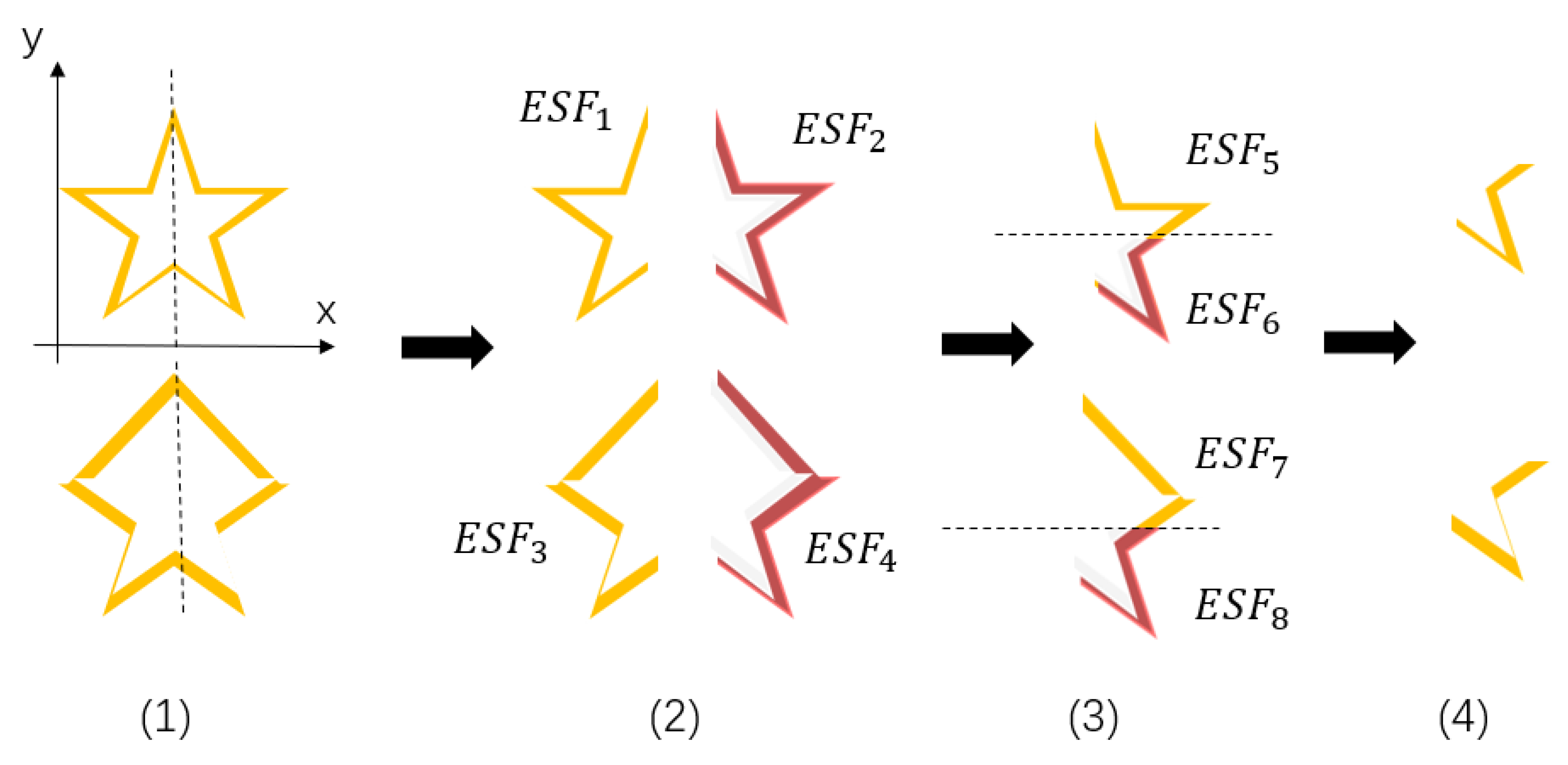
Figure 6.
Global overlapping regions extraction. Here, two two-dimensional objects with different shapes are used to represent the source point cloud and the target point cloud. Segment two point clouds simultaneously, and keep the sub-point clouds with greater similarity. in the figure represents the ESF feature of point clouds.
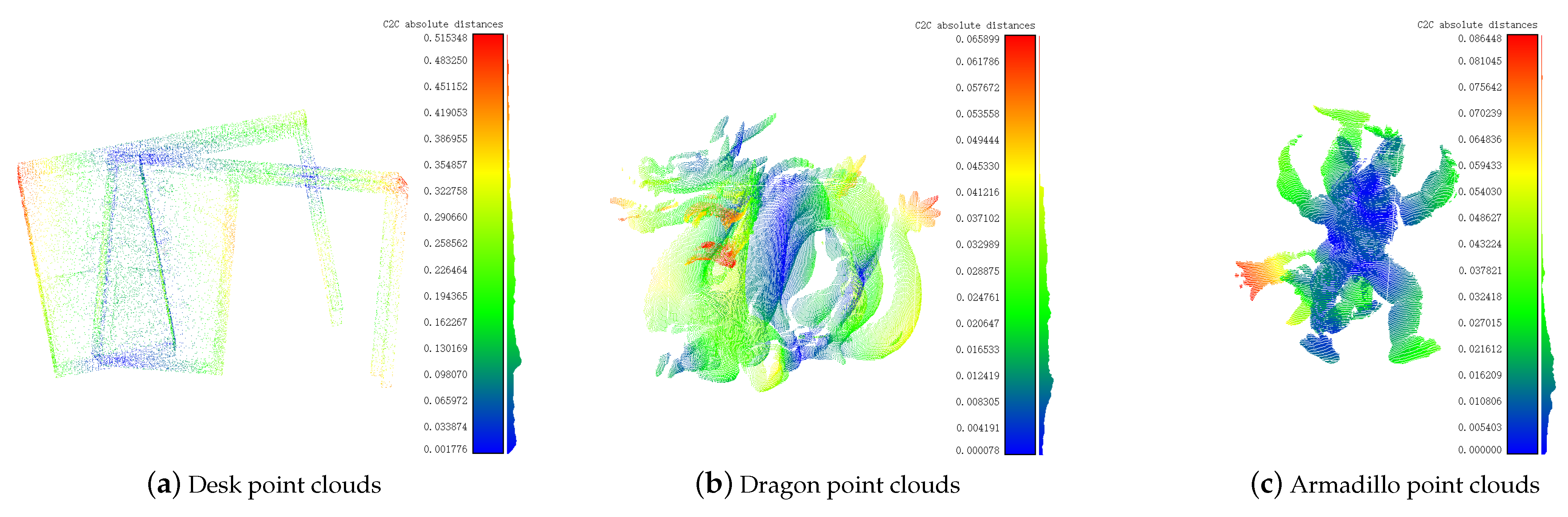
Figure 7.
Poses of original point clouds. (a), (b) and (c) are original poses of Desk, Dragon and Armadillo, respectively. The different colors in the figure represent the distance between the closest points in the point cloud, and the histogram on the right represents the specific values of the distance in meters.
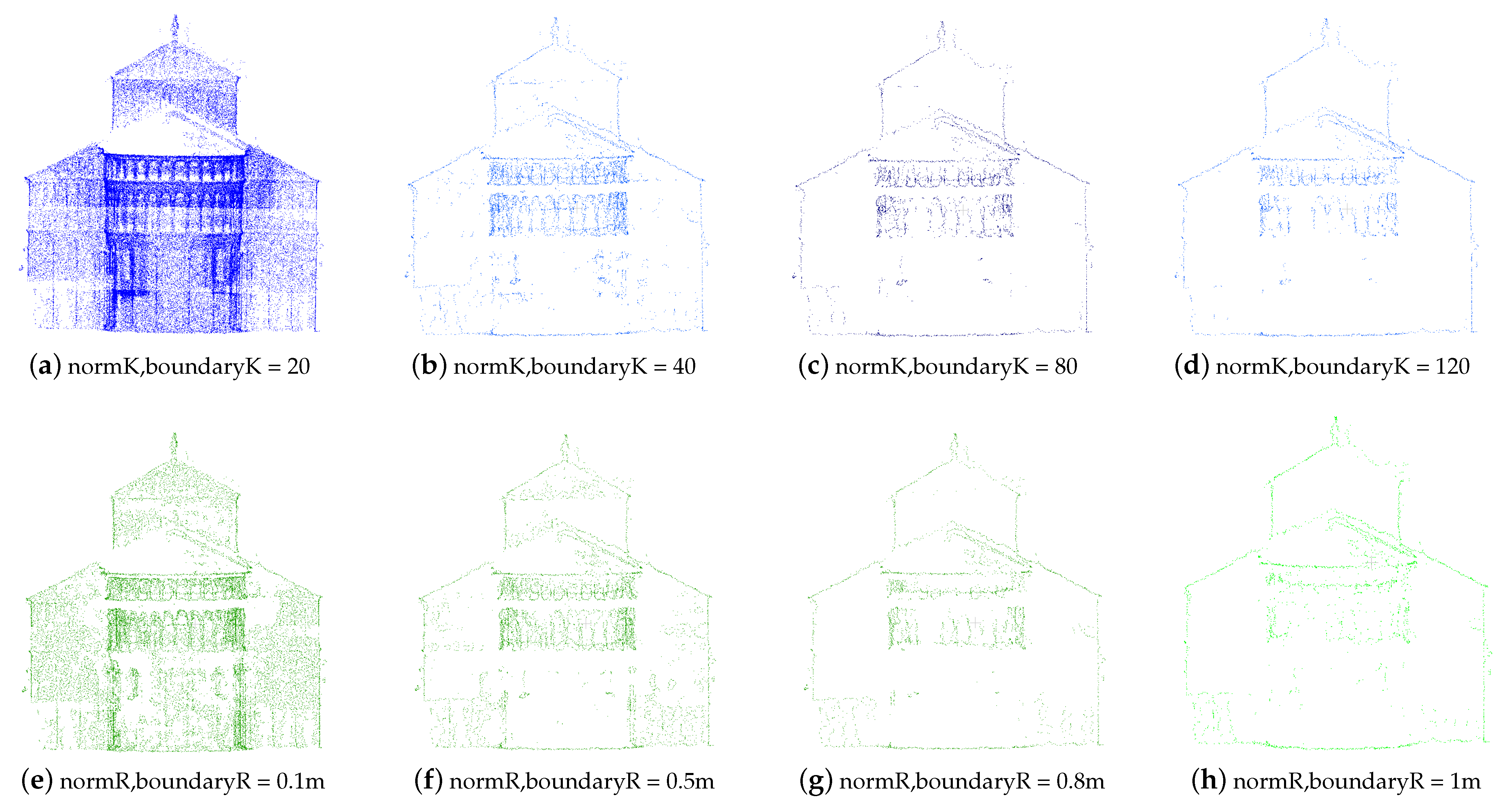
Figure 8.
The effects of boundary extraction corresponding to different neighborhood ranges and are different under two modes M, K-nearest neighbor search and R-nearest neighbor search. normK and normR are the neighborhood range of normal vector calculation, boundaryK and boundaryR are the neighborhood range of interest points.
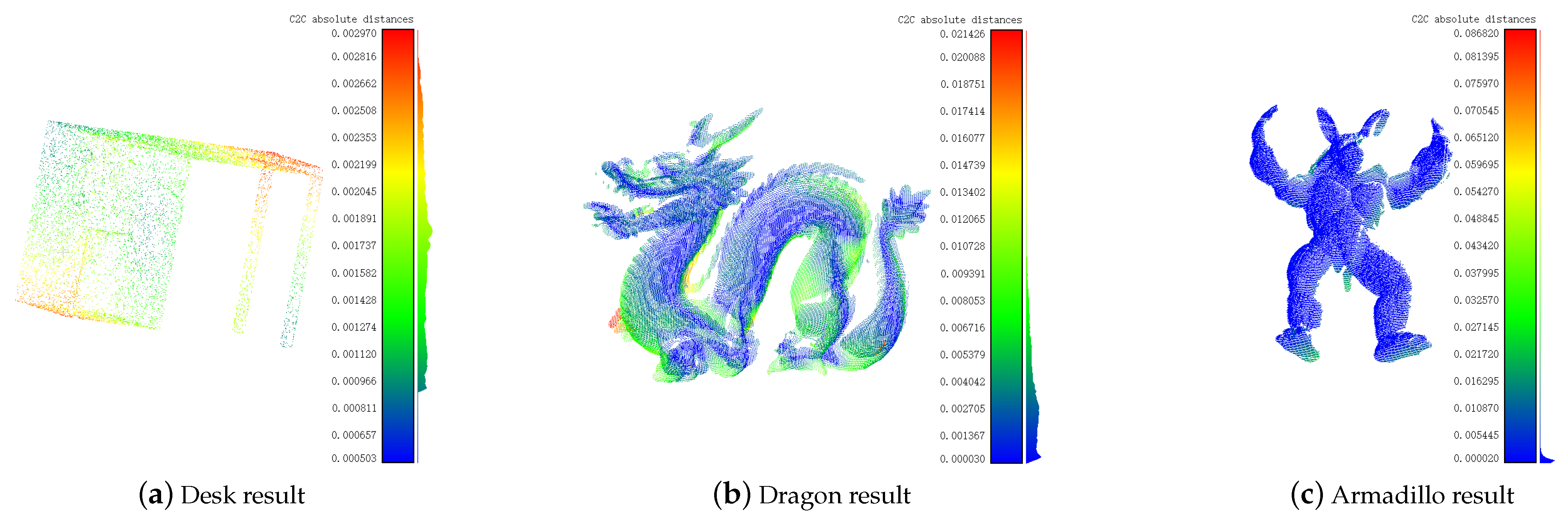
Figure 9.
The registration results of the Super Edge 4PCS algorithm on some samples. (a), (b) and (c) are the registration results of Desk, Dragon, Armadillo, respectively. Note that the distance errors of the three point clouds after registration are 0.003 m, 0.004 m, and 0.00002 m, which are smaller than tenth of the corresponding bounding box dimensions.
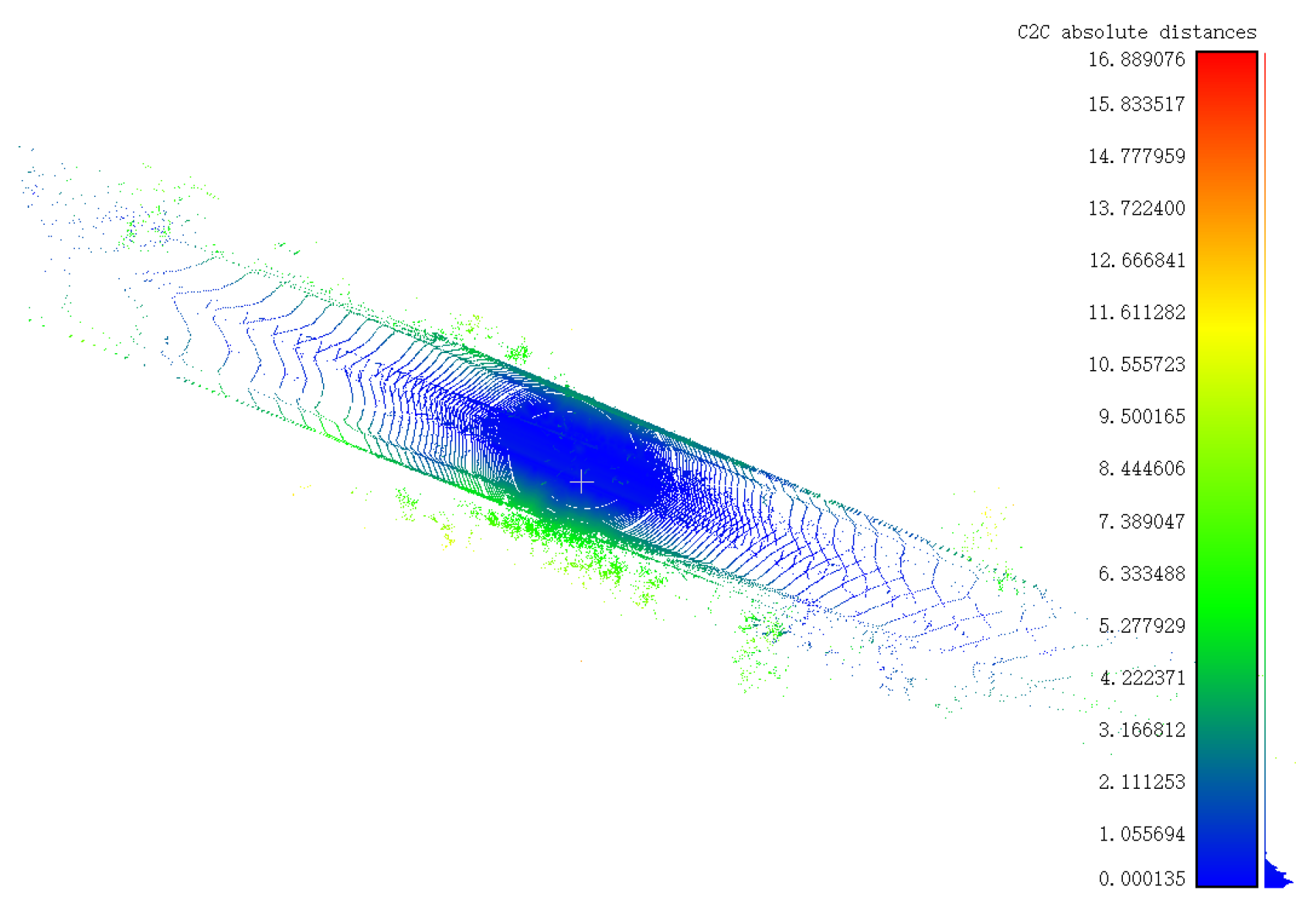
Figure 10.
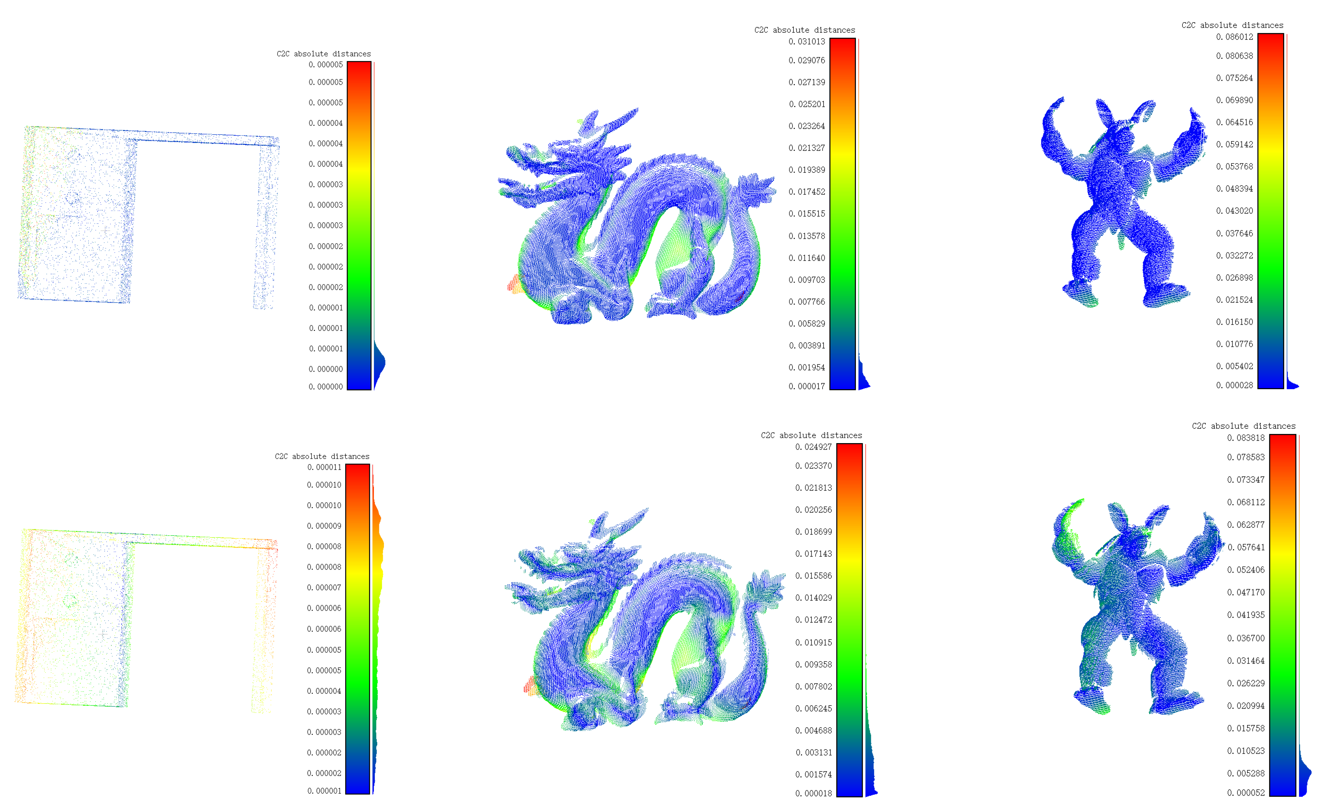
Results of ICP precise registration: the top is the results of the Super 4PCS algorithm, and the bottom is the results of Super Edge 4PCS algorithm. The main tones of three groups of point clouds toward bluey-green, which indicate that the distance error is relatively small. The specific values are reflected in the histogram on the right, and the unit is meter.
Figure 10.
Results of ICP precise registration: the top is the results of the Super 4PCS algorithm, and the bottom is the results of Super Edge 4PCS algorithm. The main tones of three groups of point clouds toward bluey-green, which indicate that the distance error is relatively small. The specific values are reflected in the histogram on the right, and the unit is meter.
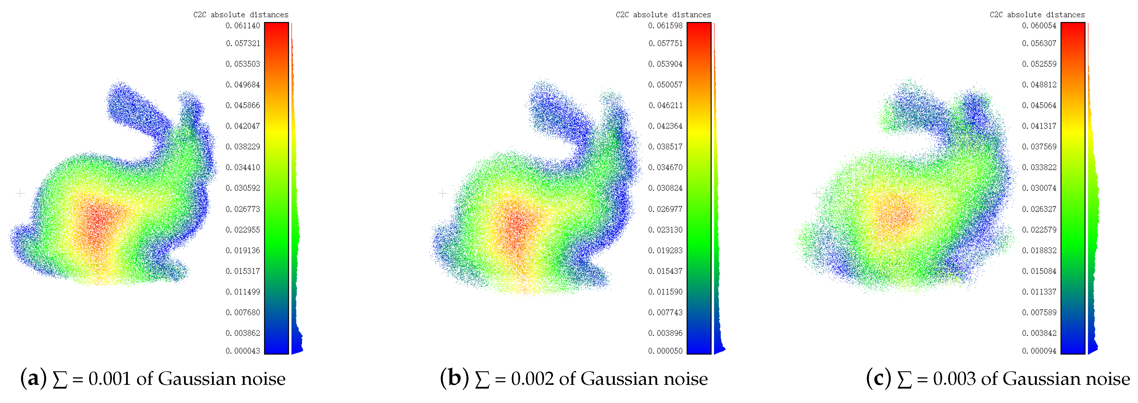
Figure 11.
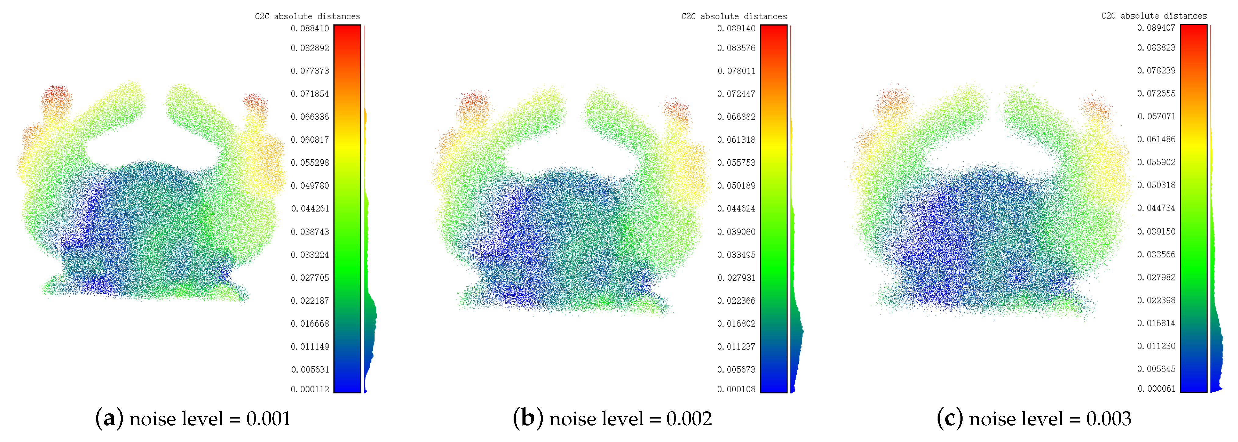
Point clouds affected by different noise levels. The noise level is measured by the different standard deviations of the added noise. (a), (b) and (c) represent the poses of source point cloud and target point cloud with noise level of 0.001, 0.002 and 0.003, respectively.
Figure 11.
Point clouds affected by different noise levels. The noise level is measured by the different standard deviations of the added noise. (a), (b) and (c) represent the poses of source point cloud and target point cloud with noise level of 0.001, 0.002 and 0.003, respectively.
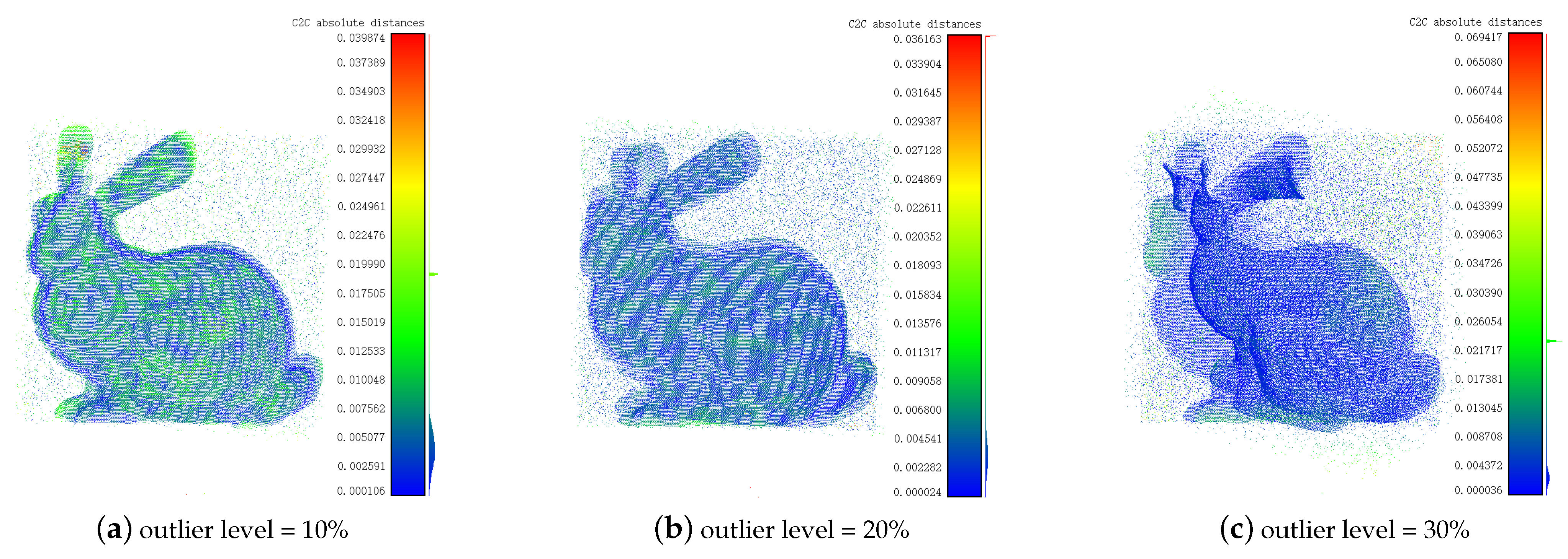
Figure 12.
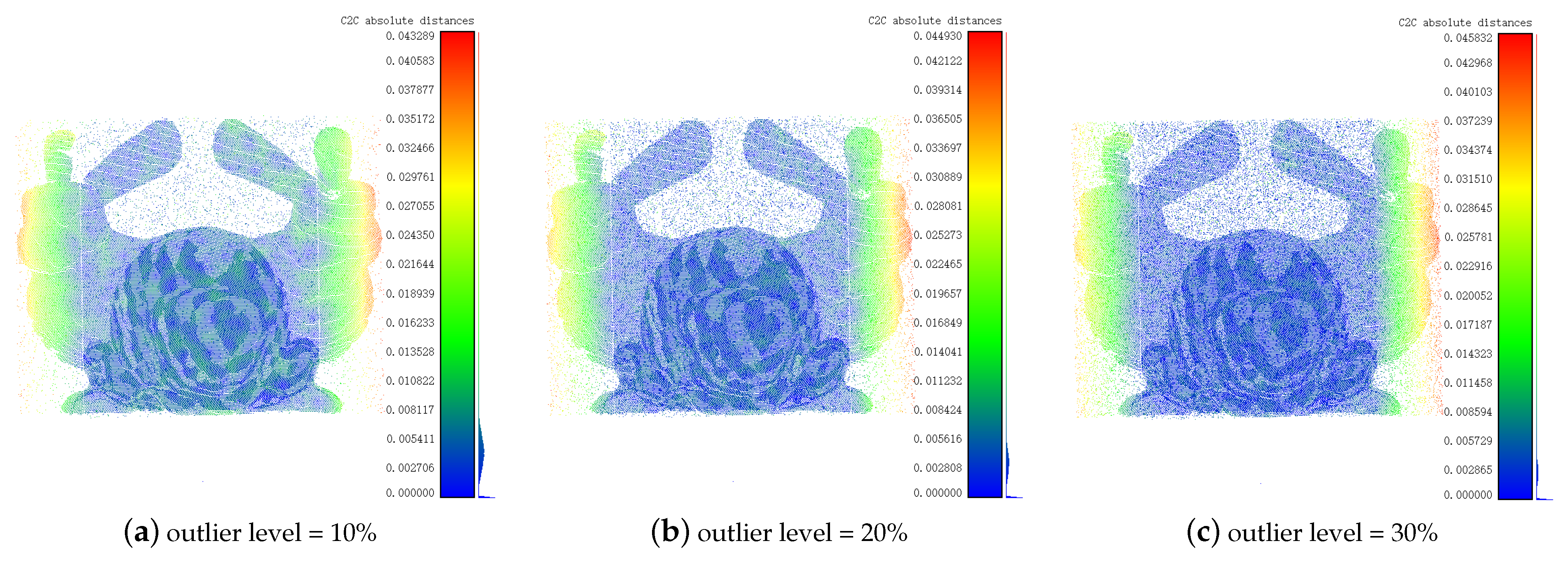
Point clouds affected by different outlier levels. The outlier level is measured by the ratio of the added outliers to the number of points in original point clouds. (a), (b) and (c) represent the poses of source point cloud and target point cloud with outlier level of 10%, 20% and 30%, respectively.
Figure 12.
Point clouds affected by different outlier levels. The outlier level is measured by the ratio of the added outliers to the number of points in original point clouds. (a), (b) and (c) represent the poses of source point cloud and target point cloud with outlier level of 10%, 20% and 30%, respectively.
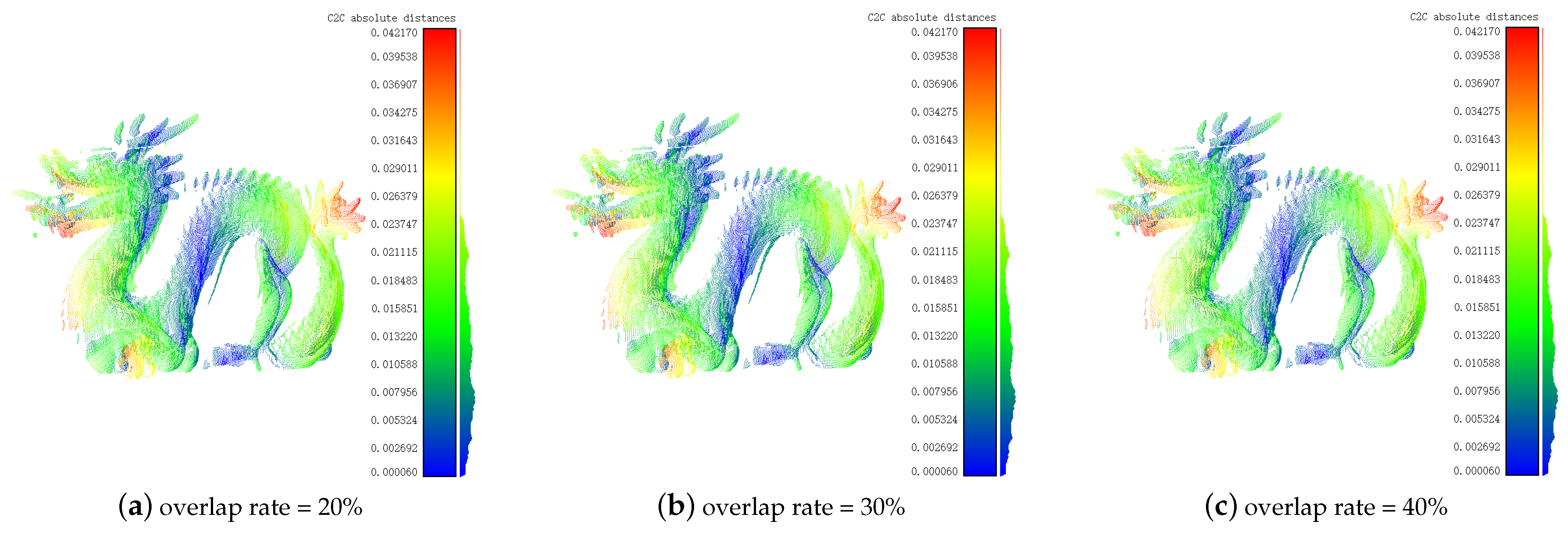
Figure 13.
Point clouds affected by different overlap rates. The overlap rate is measured by the ratio of the number of points in the overlapping regions to the number of original point clouds. (a), (b) and (c) represent the poses of source point cloud and target point cloud with overlap rate of 20%, 30% and 40%, respectively.
Figure 14.
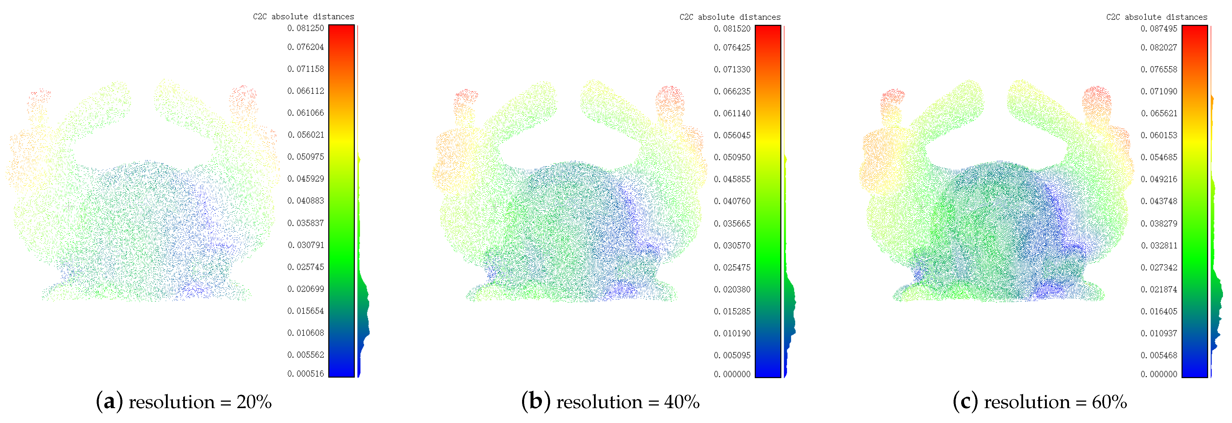
Point clouds affected by different resolutions. The resolution is measured by the ratio of the number of points in sparsed point cloud to the number of points in original point clouds. (a), (b) and (c) represent the poses of source point cloud and target point cloud with resolution of 20%, 40% and 60%, respectively.
Figure 14.
Point clouds affected by different resolutions. The resolution is measured by the ratio of the number of points in sparsed point cloud to the number of points in original point clouds. (a), (b) and (c) represent the poses of source point cloud and target point cloud with resolution of 20%, 40% and 60%, respectively.
Figure 15.
Registration results of the Super Edge 4PCS algorithm under different noise levels. represents the standard deviation of noise. The reason for the red in the center of the Bunny is that the source point cloud and the target point cloud hold hollow structures. (a), (b) and (c) represent the poses of registered point clouds under the noise level of 0.001, 0.002 and 0.003, respectively.
Figure 16.
Registration results of the Super Edge 4PCS algorithm under different outlier levels. (a), (b) and (c) represent the poses of registered point clouds under the outlier level of 10%, 20% and 30%, respectively.
Figure 16.
Registration results of the Super Edge 4PCS algorithm under different outlier levels. (a), (b) and (c) represent the poses of registered point clouds under the outlier level of 10%, 20% and 30%, respectively.
Figure 17.
Registration results of the Super Edge 4PCS algorithm under different overlap rates. These three registered point clouds are close in terms of both color and the specific value of the histogram. (a), (b) and (c) represent the poses of registered point clouds under the overlap rate of 20%, 30% and 40%, respectively.
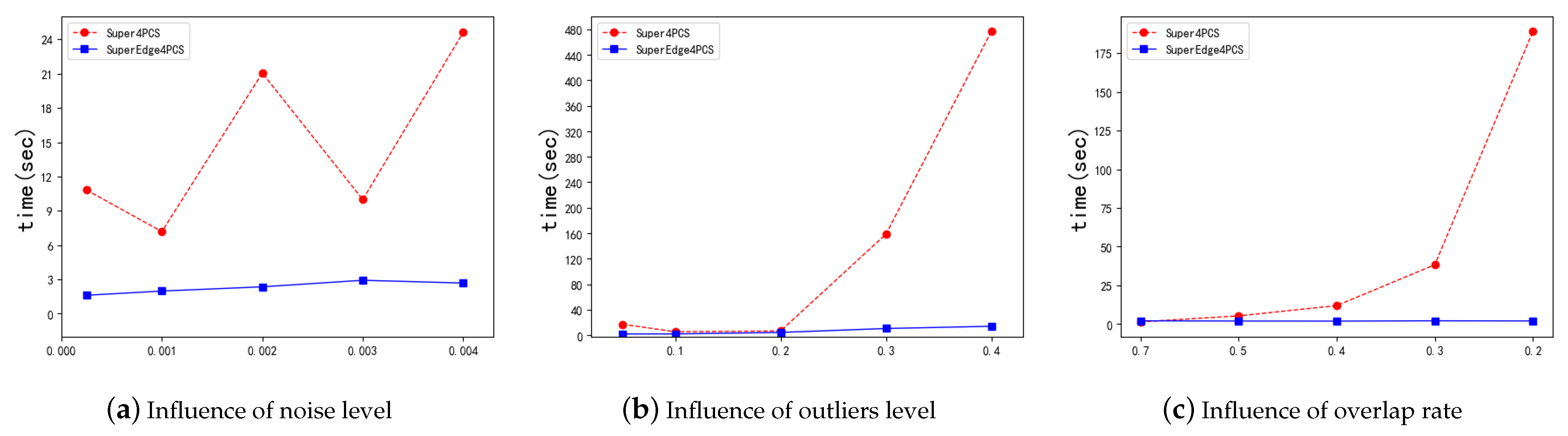
Figure 18.
Influence of noise level, outliers level and overlap rate on algorithm efficiency. The specific evaluation method is the time required for the algorithm to complete the registration under the influence of different factors. (a–c) correspond to different noise levels, outlier levels and overlap rates.
Figure 19.
Influence of different noise levels on registration accuracy (a,b) in the figure show the influence on the registration angle error and distance error. The units are degrees and meters.
Figure 19.
Influence of different noise levels on registration accuracy (a,b) in the figure show the influence on the registration angle error and distance error. The units are degrees and meters.
Figure 20.
Influence of different outlier levels on registration accuracy. (a,b) in the figure show the influence on the registration angle error and distance error. The units are degrees and meters, respectively.
Figure 20.
Influence of different outlier levels on registration accuracy. (a,b) in the figure show the influence on the registration angle error and distance error. The units are degrees and meters, respectively.
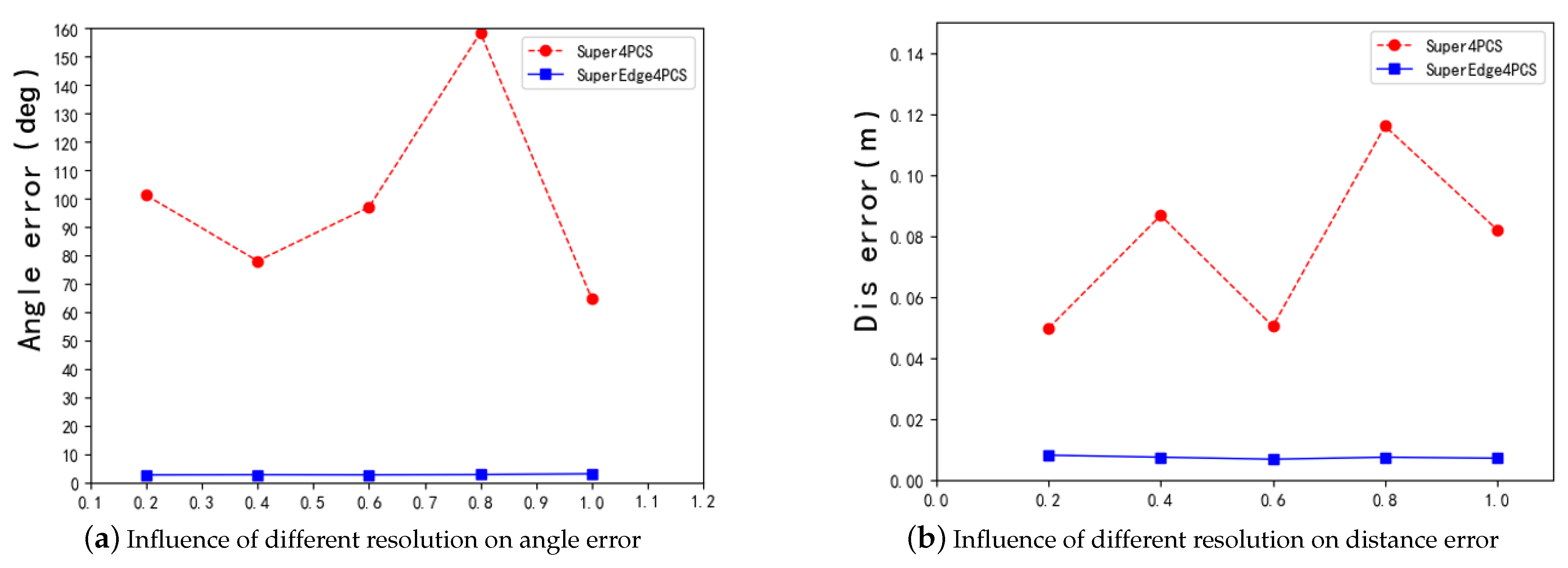
Figure 21.
Influence of different noise levels on registration accuracy. (a,b) in the figure show the influence on the registration angle error and distance error. The units are degrees and meters.
Figure 21.
Influence of different noise levels on registration accuracy. (a,b) in the figure show the influence on the registration angle error and distance error. The units are degrees and meters.
Figure 22.
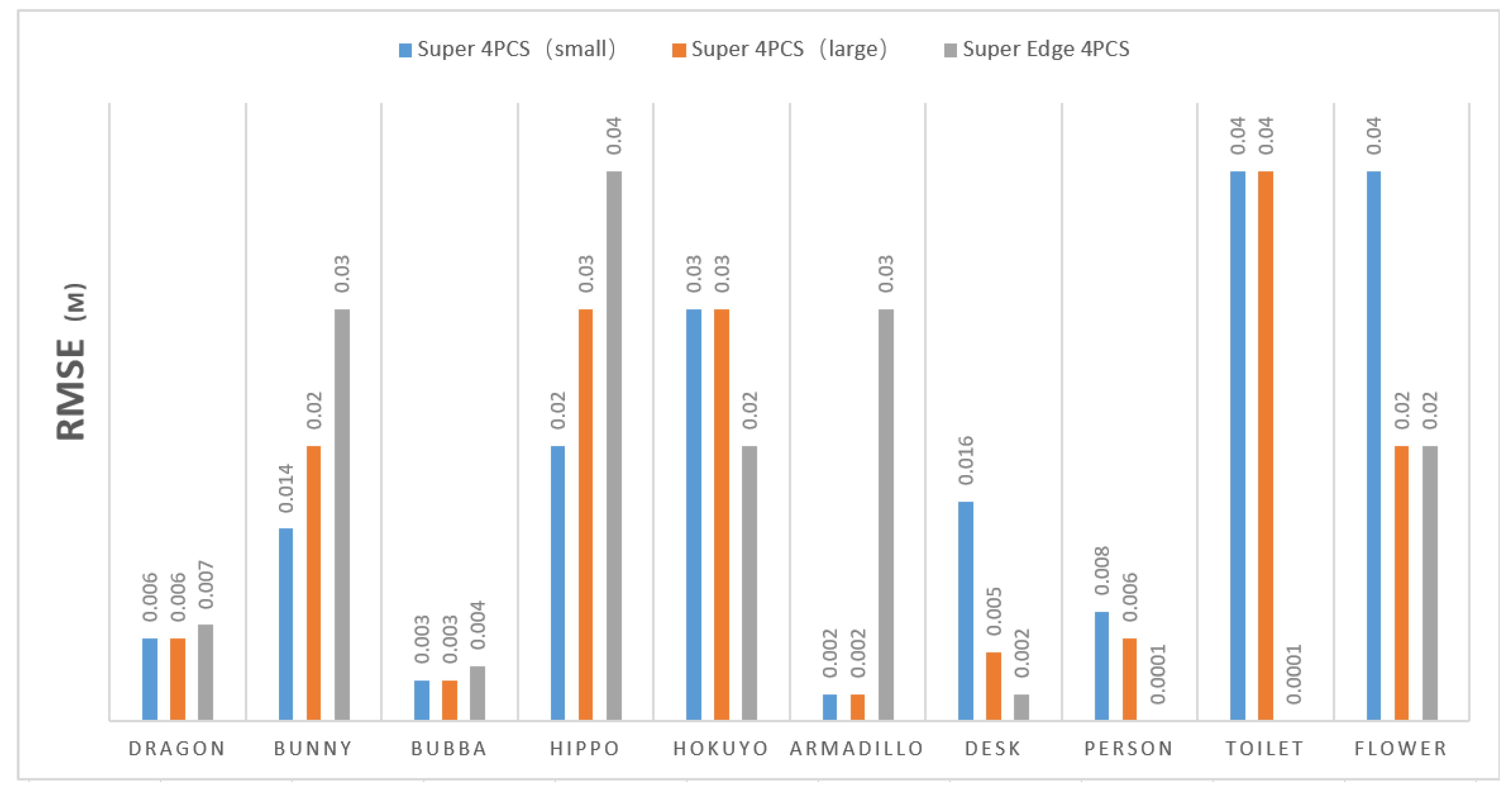
RMSEs of ten point clouds after the Super 4PCS algorithm with a large sampling size, a small sampling size and the Super Edge 4PCS algorithm. The corresponding values in the figure are compared with the bounding box dimensions of each point cloud in
Table 2, then an objective evaluation can be obtained.
Figure 22.
RMSEs of ten point clouds after the Super 4PCS algorithm with a large sampling size, a small sampling size and the Super Edge 4PCS algorithm. The corresponding values in the figure are compared with the bounding box dimensions of each point cloud in
Table 2, then an objective evaluation can be obtained.
Figure 23.
The original poses of bridge scanned in natural scene. The source and target point cloud contain a lot of noise and have uneven point distribution.
Figure 23.
The original poses of bridge scanned in natural scene. The source and target point cloud contain a lot of noise and have uneven point distribution.
Figure 24.
Registration results of the Super Edge 4PCS algorithm. The proposed algorithm gives priority to the correspondence of the dense part, which is a wrong alignment.
Figure 24.
Registration results of the Super Edge 4PCS algorithm. The proposed algorithm gives priority to the correspondence of the dense part, which is a wrong alignment.
Figure 25.
Ground-truth bridge registration. The correct registration result is that the dense parts are symmetrically distributed.
Figure 25.
Ground-truth bridge registration. The correct registration result is that the dense parts are symmetrically distributed.
Table 1.
Algorithm parameters used in the Super Edge 4PCS algorithm.
Table 1.
Algorithm parameters used in the Super Edge 4PCS algorithm.
| Code | P1 | P2 | P3 | P4 | P5 | P6 | P7 | P8 | P9 |
|---|
| parameters | M | | | h | | | | | |
| Data type | bool | int | int | int | int | int | percentage | percentage | percentage |
Table 2.
The descriptions of the experimental point clouds where View1 and View2 respectively represent the source point cloud and the target point cloud and is the length, width, and height of the bounding box.
Table 2.
The descriptions of the experimental point clouds where View1 and View2 respectively represent the source point cloud and the target point cloud and is the length, width, and height of the bounding box.
| Point Cloud | Number | Bounding Box Dimensions | Overlap Rates |
|---|
| View1(num) | View2(num) | Dimension1(m) | Dimension2(m) | Dimension3(m) |
|---|
| 1. Dragon | 34,836 | 41,841 | 0.05/0.07 | 0.16/0.16 | 0.17/0.18 | 0.5 |
| 2. Bunny | 40,256 | 40,251 | 0.09/0.1 | 0.15/0.15 | 0.17/0.18 | 0.5 |
| 3. Bubba | 59,692 | 65,438 | 0.07/0.06 | 0.08/0.08 | 0.10/0.10 | 0.8 |
| 4. Hippo | 30,519 | 21,935 | 0.31/0.30 | 0.57/0.55 | 0.65/0.62 | 0.7 |
| 5. Hokuyo | 189,202 | 190,063 | 17.41/17.66 | 27.40/28.33 | 32.46/33.39 | 0.7 |
| 6. Armadillo | 27,678 | 26,623 | 0.17/0.11 | 0.19/0.19 | 0.19/0.21 | 0.3 |
| 7. Desk | 10,000 | 10,000 | 0.79/0.79 | 1.62/1.62 | 1.80/1.80 | 0.4 |
| 8. Person | 10,000 | 10,000 | 0.51/0.51 | 0.60/0.60 | 0.79/0.79 | 0.6 |
| 9. Toilet | 10,000 | 10,000 | 1.02/1.02 | 1.39/1.39 | 1.72/1.72 | 0.8 |
| 10. Flower | 6578 | 8000 | 0.97/1.29 | 1.45/1.47 | 1.71/1.71 | 0.4 |
| 11. Bridge | 281,043 | 290,217 | 17.45/12.34 | 31.68/28.33 | 36.17/30.90 | 0.1 |
Table 3.
Parameters for registration of different point clouds.
Table 3.
Parameters for registration of different point clouds.
| Point Clouds | P1 (M) | P2 () (num) | P3 () (num) | P4 (h) (degrees) | P5 () | P6 () | P7 () | P8 (baseDis) | P9 (fDis) |
|---|
| Dragon | TRUE | 20 | 40 | 90° | 10 | 0.005 | 15% | 1% | 3% |
| Bunny | TRUE | 20 | 40 | 90° | 10 | 0.0005 | 15% | 1% | 3% |
| Bubba | TRUE | 20 | 40 | 90° | 10 | 0.005 | 15% | 1% | 3% |
| Hippo | TRUE | 20 | 40 | 90° | 10 | 0.0007 | 15% | 18.5% | 3% |
| Hokuyo | TRUE | 20 | 40 | 90° | 10 | 0.05 | 15% | 2.5% | 3% |
| Armadillo | TRUE | 20 | 40 | 90° | 10 | 0.0005 | 15% | 14.5% | 3% |
| Desk | TRUE | 20 | 40 | 90° | 10 | 0.001 | 15% | 1% | 3% |
| Person | TRUE | 20 | 40 | 90° | 10 | 0.001 | 15% | 1% | 3% |
| Toilet | TRUE | 20 | 40 | 90° | 10 | 0.001 | 15% | 1% | 3% |
| Flower | TRUE | 20 | 40 | 90° | 0.005 | 0.001 | 15% | 1% | 3% |
Table 4.
RMSEs between point clouds after ICP algorithm. Dimension 1, 2, 3 represent the length, width, and height of the bounding box of each point cloud, respectively.
Table 4.
RMSEs between point clouds after ICP algorithm. Dimension 1, 2, 3 represent the length, width, and height of the bounding box of each point cloud, respectively.
| Point Cloud | Desk | Dragon | Armadillo |
|---|
| Super 4PCS (m) | 0.001 | 0.004 | 0.004 |
| Super Edge 4PCS (m) | 4 × | 0.005 | 0.006 |
| Dimension1 (m) | 0.79 | 0.05 | 0.17 |
| Dimension2 (m) | 1.62 | 0.16 | 0.19 |
| Dimension3 (m) | 1.80 | 0.17 | 0.19 |
Table 5.
The running time of sub stage of Super 4PCS and Super Edge 4PCS in different samples. CSE and CSV represent the congruent sets extraction and congruent sets verification, respectively.
Table 5.
The running time of sub stage of Super 4PCS and Super Edge 4PCS in different samples. CSE and CSV represent the congruent sets extraction and congruent sets verification, respectively.
| | | CSE | CSV | |
|---|
| Point | Sample | SE4PCS (s) | S4PCS (s) | S4PCS (s) | SE4PCS (s) | S4PCS (s) | S4PCS (s) | Overlap |
| Cloud | Size (num) | | (Small) | (Large) | | (Small) | (Large) | Rate |
| Flower | 7289 | 0.9 | 1.5 | 8.9 | 0.04 | 0.008 | 0.4 | 0.4 |
| Desk | 10,000 | 0.4 | 9.6 | 35.3 | 0.06 | 0.3 | 2.9 | 0.4 |
| Person | 10,000 | 0.4 | 2.4 | 8.1 | 0.06 | 0.4 | 4.1 | 0.6 |
| Toilet | 10,000 | 0.4 | 0.5 | 1.5 | 0.06 | 0.02 | 0.3 | 0.8 |
| Bubba | 62,565 | 2.0 | 0.6 | 1.5 | 0.4 | 0.3 | 4.4 | 0.8 |
| Dragon | 38,338 | 2.6 | 8.2 | 16.2 | 0.2 | 1.2 | 9.2 | 0.5 |
| Bunny | 40,253 | 1.1 | 2.2 | 7.0 | 0.2 | 0.1 | 1.8 | 0.5 |
| Average | - | 1.1 | 3.6 | 11.2 | 0.1 | 0.3 | 3.3 | - |
Table 6.
Statistics of the running time and registration error of the two algorithms in ten point clouds. TS% and DR represent the improvement in calculation time and accuracy of the proposed algorithm compared to the Super 4PCS algorithm, respectively.
Table 6.
Statistics of the running time and registration error of the two algorithms in ten point clouds. TS% and DR represent the improvement in calculation time and accuracy of the proposed algorithm compared to the Super 4PCS algorithm, respectively.
| Model | Super 4PCS | Super Edge 4PCS | Comparison |
|---|
| Sampling Size (num) | (s) | (m) | (s) | (m) | % | (m) |
|---|
| Dragon | 680/1080 | 11.2/26.4 | 0.006/0.006 | 1.3 | 0.007 | 88.3%/95.0% | −0.001/−0.001 |
| Bunny | 522/953 | 6.0/13.9 | 0.014/0.02 | 1.6 | 0.03 | 73.2%/88.6% | −0.01/−0.01 |
| Bubba | 732/1378 | 1.6/6.0 | 0.003/0.003 | 2.4 | 0.004 | −51.3%/60.2% | −0.001/−0.001 |
| Hippo | 220/413 | 0.4/1.9 | 0.02/0.03 | 1.0 | 0.04 | 88.9%/97.9% | −0.02/−0.01 |
| Hokuyo | 1300/2000 | 93.5/770.1 | 0.03/0.03 | 6.0 | 0.02 | 93.7%/99.2% | 0.01/0.01 |
| Armadillo | 634/1080 | 55.9/264.1 | 0.002/0.002 | 1.3 | 0.03 | 97.7%/99.5% | −0.02/−0.02 |
| Desk | 407/913 | 12.2/42.2 | 0.016/0.005 | 0.4 | 0.002 | 96.6%/99.0% | 0.01/0.003 |
| Person | 513/871 | 3.6/11.9 | 0.008/0.006 | 0.4 | 3.17 × 10 −7 | 88.2%/96.5% | 0.008/0.006 |
| Toilet | 431/796 | 0.7/1.8 | 0.04/0.04 | 0.4 | 3.6 × 10 −7 | 35.9%/75.7% | 0.04/−0.04 |
| Flower | 213/527 | 3.2/11.4 | 0.04/0.02 | 1.6 | 0.02 | 51.2%/86.1% | 0.03/0.001 |
| Average | - | 18.8/114.9 | 0.02/0.02 | 1.6 | 0.01 | 66.2%/89.8% | 0.005/−0.003 |


