Abstract
Clutter suppression in heterogeneous environments is a serious challenge for airborne radar. To address this problem, a matrix-manifold-based clutter suppression method is proposed. First, the distributions of training data in heterogeneous environments are analyzed, while the received data are characterized on a Riemannian manifold of Hermitian positive definite matrices. It is indicated that the training data with different distributions with the same power are separated, whereas data with the same distribution are closer together. This implies that the underlying geometry of the data can be better revealed by manifolds than by Euclidean space. Based on these properties, homogeneous training data are selected by establishing a binary hypothesis test such that the negative effects of the use of heterogeneous samples are alleviated. Moreover, as exploiting a geometric metric on manifolds to reveal the underlying information of data, experimental results on both simulated and real data validate that the proposed method has a superior performance with small sample support.
1. Introduction
Airborne radar plays an important role in detecting aircraft, ships, and vehicles at long ranges [1]. However, due to the platform motion, slowly moving targets are easily masked by strong clutter; hence, clutter suppression is a challenging problem for airborne radar to overcome [2,3]. Traditional typical clutter suppression methods include displaced phase center antenna (DPCA) [4] and along-track interferometry (ATI) [5]. The DPCA technique requires a very stringent constraint on the baseline between channels, limiting the clutter suppression performance. Then, to enable superior clutter suppression performance, space-time adaptive processing (STAP) was developed [6,7,8]. It is well known that STAP involves the design of a space-time adaptive filter, which requires the accurate estimation of the clutter covariance matrix (CCM) of the cell under test (CUT) [9]. Generally, training data that share the same statistical characteristics with the data of CUT are used to estimate the CCM. The conventional sample matrix inverse (SMI) approach performs well when the number of training samples is greater than two times the dimensionality of STAP [10]. Unfortunately, this is restricted because the large independent and identical distribution (i.i.d) sample requirement will not usually hold in heterogeneous environments [11]. Worse still, training data are usually contaminated by outliers (i.e., discrete clutter), resulting in remarkable clutter suppression performance degradation.
To address this problem, sufficient research has been performed. Trimming algorithms were designed to eliminate the contaminated training samples. Many algorithms concentrate on an effective non-homogeneity detector (NHD) [12,13] in which the generalized internal product (GIP) and the adaptive power residue (APR) are two important criteria. Since certain NHDs depend on the training data used, to mitigate the finite sample effect, improved methods were proposed, e.g., a new type of GIP detector based on diagonal loading (LGIP) was reported in [14] and a cyclic training sample selection and cancellation (CTSSC) algorithm was proposed in [15]. Conversely, sub-optimal algorithms that require fewer samples have been devised. For instance, reduced-dimension [16,17] (e.g., loaded sample matrix inversion (LSMI) [6], 3DT [17]) and reduced-rank algorithms [18,19] (e.g., methods exploiting structural information) were proposed to diminish the demand for samples. These algorithms rely on specific assumptions about the data’s statistical properties and suffer from performance loss [9]. In addition, for the reduced-rank methods, samples with two times of rank are also needed. To further reduce the demand for samples and handle the problem of contaminated training samples, a direct data domain least squares (D3LS) algorithm operating on a snapshot-by-snapshot basis was proposed in [20]. However, the benefit of not requiring the training data depends on the cost of the reduced system degree of freedom (DoF). Afterward, knowledge-aided STAP algorithms provide an alternative solution to reduce the required samples by exploiting a priori knowledge [21]. Unfortunately, it is not easy to obtain precise knowledge. Recently, a sparse recovery-based STAP (SR-STAP) algorithm was proposed [22], but this algorithm depends on the accuracy of sparse model and has a powerful calculating ability. These algorithms are considered in Euclidean space and do not make use of the data structure, leading to subpar performance. Recently, the relevance of matrix information geometry methods for radar signal processing has been of focus and demonstrated [23,24]. These methods exploit the non-linear geometry of matrix manifolds and show advantages in signal processing. For example, to avoid the drawbacks of Doppler processing with few pulses, a new strategy for radar detection using matrix CFAR on the symmetric positive definite covariance matrices of data was reported [25]. Furthermore, approaches based on the parameter tuning of regularized covariance matrix estimators were provided in [26,27], and median-based detectors with a manifold filter was applied in [28] to improve the target detection performance. In [29], a novel technique based on Riemannian geometry for synthetic aperture radar was derived, which could achieve accurate target recognition performance. In [30], utilizing a gradient descent algorithm on manifolds, a random matrix theory-based method was proposed and used for target classification. Meanwhile, there have been several studies concerning clutter suppression based on manifolds, i.e., a training data selection method via geometric barycenter was investigated in [31] and an algorithm based on the Karcher barycenter was developed in [32]. However, the aforementioned training data selection method did not consider small sample support. The algorithm uses the Riemannian barycenter to improve the clutter suppression performance, which requires iteration, and the computational burden is extremely heavy. Moreover, it does not consider heterogeneous environments. Briefly, the existing manifolds-based clutter suppression algorithms cannot consider small sample support and the existence of discrete clutter in training data at the same time. This motivated the current authors to conduct the investigation described in this paper.
To suppress heterogeneous clutter for airborne radar, a matrix-manifolds-based method is proposed. First, the received data are characterized on a Riemannian manifold of Hermitian positive definite (HPD) matrices. Then, the distributions of the training data are analyzed when there are few homogeneous samples and discrete clutter points in heterogeneous environments. It is indicated that the training data with different distributions and the same power are separated on manifolds, whereas those with the same distribution are close. This implies that the underlying geometry of the data can be better revealed by manifolds than by Euclidean space. Based on these properties, homogeneous samples with CUT can be selected by establishing a binary hypothesis test. Moreover, the clutter covariance matrix estimation problem is converted into the geometric centroid optimization on manifolds. To obtain an accurate and robust centroid, the improvement factor (IF), robustness to corrupted training data, and computational efficiency are proposed to evaluate the dissimilarity metrics, combined with practical needs. The superiority of the proposed method is demonstrated by comparing the competing approaches in the experiment. Our results show that the most homogeneous training data can be extracted effectively, and the requirement of the samples can be decreased.
Notations: Throughout this paper, scalar quantities are denoted with the italic typeface. Lowercase italic boldface quantities denote vectors and uppercase italic boldface quantities denote matrices. denotes the conjugate transpose operation. denotes the norm and represents that is a positive definite matrix. denotes the diagonal operation, denotes the identity matrix, denotes the trace of a matrix, denotes the statistical expectation, and denotes the kronecker product.
2. Array Signal Model and Problem Formulation
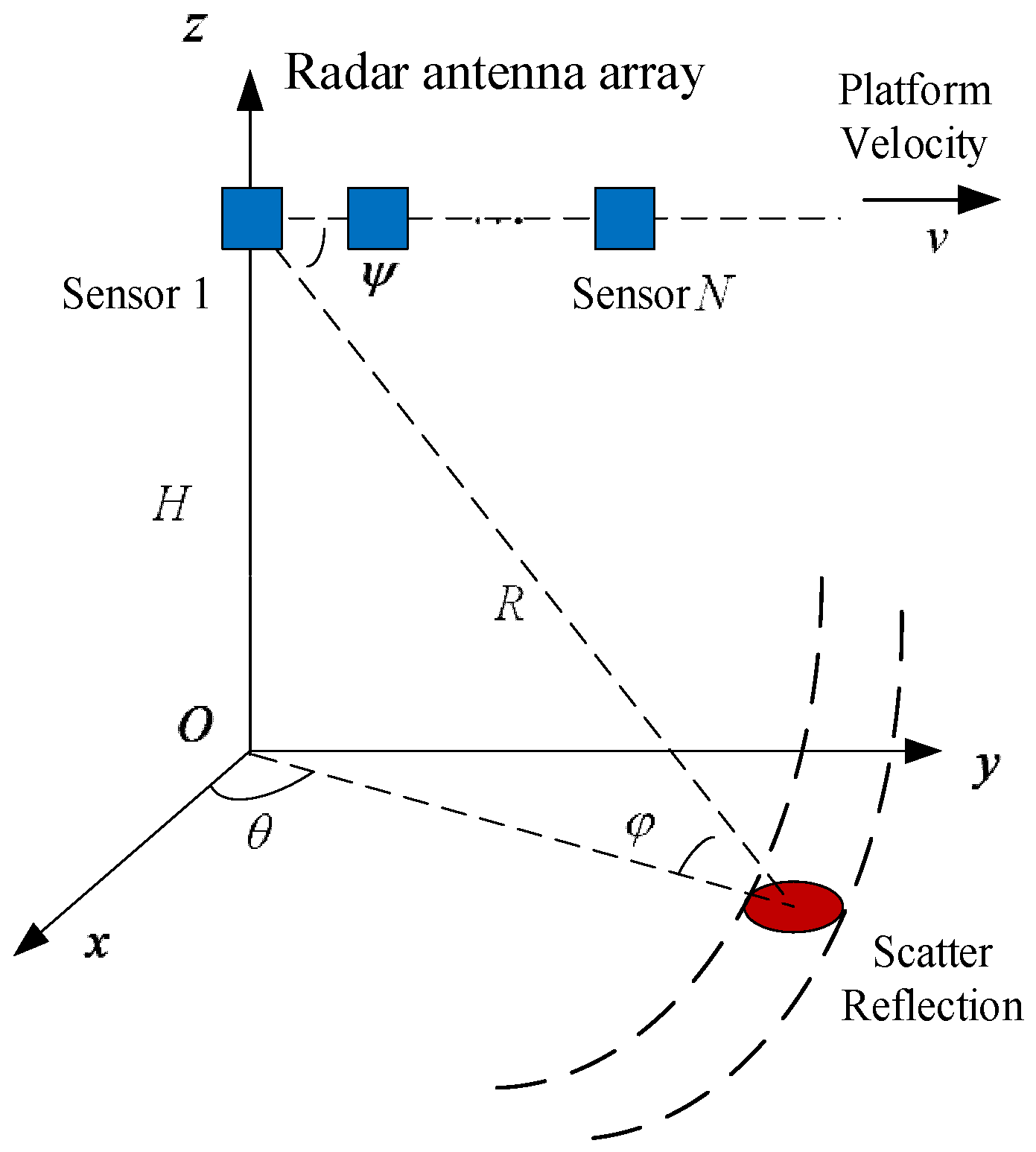
Consider a side-looking airborne radar system with antenna elements in a uniform linear array, as shown in Figure 1. The platform travels with a velocity , and the scatter point on the ground has an
azimuth angle , and an elevation angle . Each sensor in the array transmits pulses during a coherent processing interval. The radar operating wavelength is .

Figure 1.
Geometric model of airborne radar system.
In an airborne STAP radar system, the space-time snapshot received by sensors in the range bin encompasses different components: the target signal , the clutter patch echo , the interference signal (only discrete clutter is considered here, for notational convenience, it is dubbed as an outlier) and the noise ,
where and indicate the number of clutter patches and outliers, and represent the complex amplitude of the clutter patch and outliers, is the scatter reflection coefficient of the target signal, and represents the steering vector of the target signal
and
representing the Doppler and spatial steering vectors of the target, respectively, where , is the pulse repetition interval, , and is the inter-element spacing between antenna elements. Correspondingly, and are the steering vectors of the clutter patch and outliers, respectively.
We denote the training data in the range cell without targets as . Then, to form the space-time adaptive filter,
the CCM estimated by SMI, which has been widely used, takes the form
where is the number of training data and is the CCM in the range bin.
After applying the space-time filter, the improvement factor (IF) [9] is usually used to assess the clutter suppression performance,
where and are the output signal-clutter plus noise to power
ratio (SCNR) and input SCNR, respectively. The noise power is , represents the clutter to noise ratio, and is the CCM in the CUT. The adaptive weights for clutter suppression can be calculated by
Note that conventional clutter suppression methods based on SMI achieve satisfactory performance when there are sufficient homogeneous samples. However, in heterogeneous environments, due to the shortage of homogeneous samples, inaccurate CCM estimation leads to remarkable clutter suppression performance loss. Hence, in view of this, improved clutter suppression methods in heterogeneous environments should be investigated.
3. Training Data Selection Based on Manifolds in Heterogeneous Environments
In this section, a Riemannian manifold of HPD matrices is established first. Then, the properties of the distribution of training data in heterogeneous environments are discussed. Based on these properties, training data are selected using a binary hypothesis test.
3.1. The Establishment of a Matrix Manifold
Notice that the CCM estimated in (5) can also be viewed as the arithmetic mean of the sample matrices in Euclidean space, which is generalized by the following optimization problem [33]
where represents the distance in Euclidean space, and is the -dimensional linear space spanned by the observed
matrices. The weight (with and ) allows the weighting of the training data in each range bin. Moreover, the distance that is commonly used in (8) can also be reformulated as . Unfortunately, it only focuses on the signal power and does not make use of the data structure. To overcome this drawback, we try to focus on the properties of data. Herein, the covariance matrix that can implicitly capture the second-order statistical characteristics of the received data in each range bin is employed. Specifically, the CCM in each range bin is devised as the following
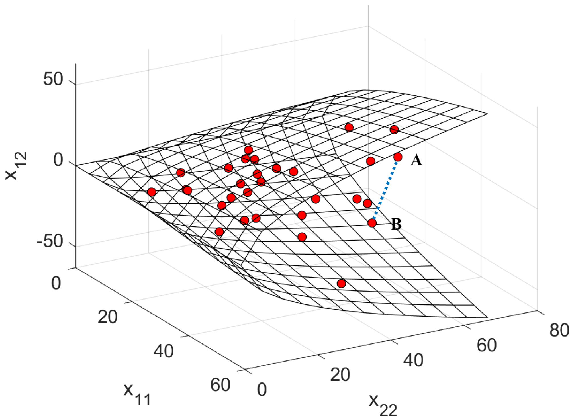
where the coefficient can be obtained by the average over time instead of statistical expectation, and represents the slow time. The CCM (not only , but also ) has a positive semi-definiteness property, thus the space constituted by the covariance matrices is not closed under addition and scalar products (e.g., multiplying a positive definite matrix with a negative scalar makes it a negative definite) [34]. Hence, the space of covariance matrices is not linear. Furthermore, the CCM estimation through Euclidean space (a linear space) in (8) is not optimal. To demonstrate this further, we generate a set of 22 positive definite matrices according to the Wishart distribution and present the space constituted by these covariance matrices in Figure 2.
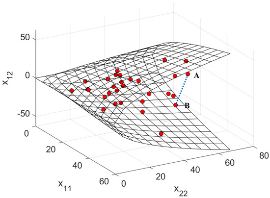
Figure 2.
The space of a set of 2 2 covariance matrices.
Herein, represent the coordinate, and the red circles represent covariance matrices. As observed, the Euclidean distance (the blue dotted line) between two points (point A and B) of the CCMs is neither informative nor accurate. This confirms the subpar performance of the conventional estimation methods in Euclidean space.
Fortunately, a manifold is a space that is diffeomorphic to a Euclidean
space. Intuitively speaking, a manifold is a nonlinear space, and it has a
locally linear structure. As seen in Figure 2,
the space of the covariance matrices lacks a global linear structure but has a
local linear structure. Moreover, geometric methods on manifolds are useful
methods for handling the problem in nonlinear space. Therefore, it is logical
to consider our problem on manifolds. Based on this idea, we established a
Riemannian manifold of HPD matrices (also referred to as the “matrix manifold”)
to handle the clutter suppression problem in heterogeneous environments. First,
the space of Hermitian matrices constituted by the set of matrices is expressed as
where is the dimension and the space of all the HPD
matrices can be given by
where represents the positive definite matrix.
The
space is a manifold endowed with a Riemannian distance.
The so-called distance on manifold between and is the infimum of lengths of curves connecting them
where is the length of , which is a sufficiently smooth curve in .
3.2. The Properties of the Distribution of Training Data in Heterogeneous Environments
Based on the aforementioned section, the covariance matrices of training data can be described as different points on manifolds. Then, to reflect the underlying geometry of the data better, the distributions of these points in heterogeneous environments are analyzed in this subsection. Herein, to analyze the characteristics of training data, it is necessary to map high-dimensional data into two dimensions, while maintaining the local structure of the data. Therefore, the manifold learning algorithm-tSNE [35] is exploited to discuss the distribution of training data.
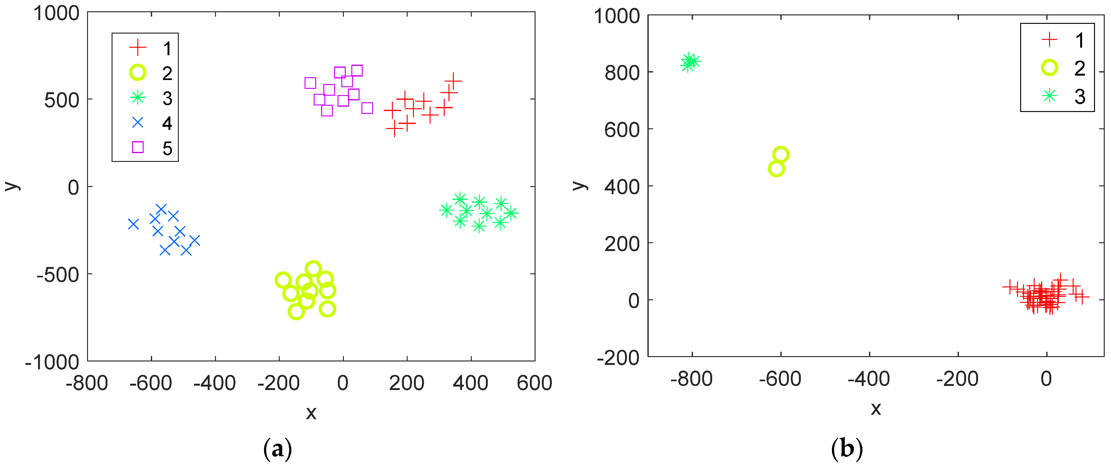
Both the typical cases in heterogeneous environments that will affect the clutter suppression performance of STAP are discussed. The first case is that the training data obey different distributions with CUT, and for the other, the training data are corrupted by outliers. For ease of discussion, a standard STAP system that employs a uniform linear array with half-wavelength inner spacing is considered. By applying the t-SNE algorithm, the distributions of covariance matrices in heterogeneous environments are provided in Figure 3. In the scene, there are 10 array elements, 8 pulses in a coherent pulse interval (CPI), and 50 range bins. We assume that the data of different range bins obey different distributions but have the same power in Figure 3a. For the sake of brevity, we label the data in the range bins which obey K, normal, lognormal, Weibull, and Rayleigh distribution as 1 to 5, respectively. Moreover, the covariance matrix in each range bin is constructed by (9). Therefore, different points in Figure 3a correspond to the labelled covariance matrices of different range bins. Similarly, the case of training samples contaminated by outliers in the training dataset is considered in Figure 3b. In this case, the clutter data of 50 range bins all obey a normal distribution, but there are five outliers among them. Specifically, the data in the range bins from to are homogeneous training data, and their power is 5 dB. However, the clutter power in the range bin from to and that in the range bins from to are 10 dB and 15 dB, respectively. Correspondingly, the covariance matrices of different range bins are also obtained according to (9). Similarly, the range bins of homogeneous training data (range bins from to ) are labeled as 1 and the range bins of training samples contaminated by different outliers are labeled 2 (range bins from to ) to 3 (range bins from to ).

Figure 3.
The distribution of covariance matrices constituted by training samples in heterogeneous environments: (a) covariance matrices with different distributions; (b) covariance matrices with the existence of outliers.
From Figure 3, as observed, the points of training data with different distributions are separated and those with the same distribution are closer together. Similarly, the points of the homogeneous samples are close, whereas the outliers are far away from the homogeneous samples. The results imply that, while ignoring the signal power, the underlying geometry of the data (usually discarded by the traditional method in Euclidean space) can be better revealed by the manifold. These properties may be exploited to select homogeneous samples and CCM estimation in heterogeneous environments.
3.3. The Screening of Training Data
We assume that the statistical characteristics of data in a presumed range cell (maybe the cell adjacent to CUT and several guard cells are set) are the same as the statistical characteristics of CUT, and denote the CCM of the presumed cell as . Thus, the training data sharing the same
distribution can be selected by a binary classification problem. We denote the
homogeneous data set as and the heterogeneous data set as , respectively. Then, the screening problem of
training data is transformed into the following binary hypothesis test
The decision rules for problem (13) are based on the Euclidean distance between different points after the manifold learning algorithm, that is
The threshold can be set by guaranteeing a given probability of classifying data as heterogeneous when they are homogeneous. In our method, the threshold is obtained through 100 independent Monte-Carlo trails. After the screening of training data, the number of homogeneous samples is usually far less than the DoF. Therefore, the clutter suppression with limited samples is investigated in the next section.
4. Clutter Suppression Based on Matrix Manifolds
Although the operation of selected training data removes the influence of heterogeneous samples, the number of available samples is also reduced. In this section, we propose a novel clutter suppression method for STAP where the CCM estimation problem is converted into the geometric centroid optimization on manifolds. To obtain a more accurate and robust centroid, criteria are proposed to evaluate the dissimilarity metrics, combining the practical needs. Moreover, a specific scheme of clutter suppression on manifolds is given.
4.1. Clutter Covariance Matrix Estimation on Matrix Manifolds
As stated before, the space of covariance matrices is nonlinear, but the existing methods in Euclidean space search the estimated CCM in a single linear space constraint (as shown in (8)). Meanwhile, the manifold is nonlinear and shows advantages to reflect the underlying geometry of the data. Therefore, when generalizing the constraint to a manifold, the estimation problem can be performed directly on the nonlinear search space. As such, the CCM estimation in our scenario is recast as the following unconstrained optimization problem
where represents the dissimilarity metric on manifolds.
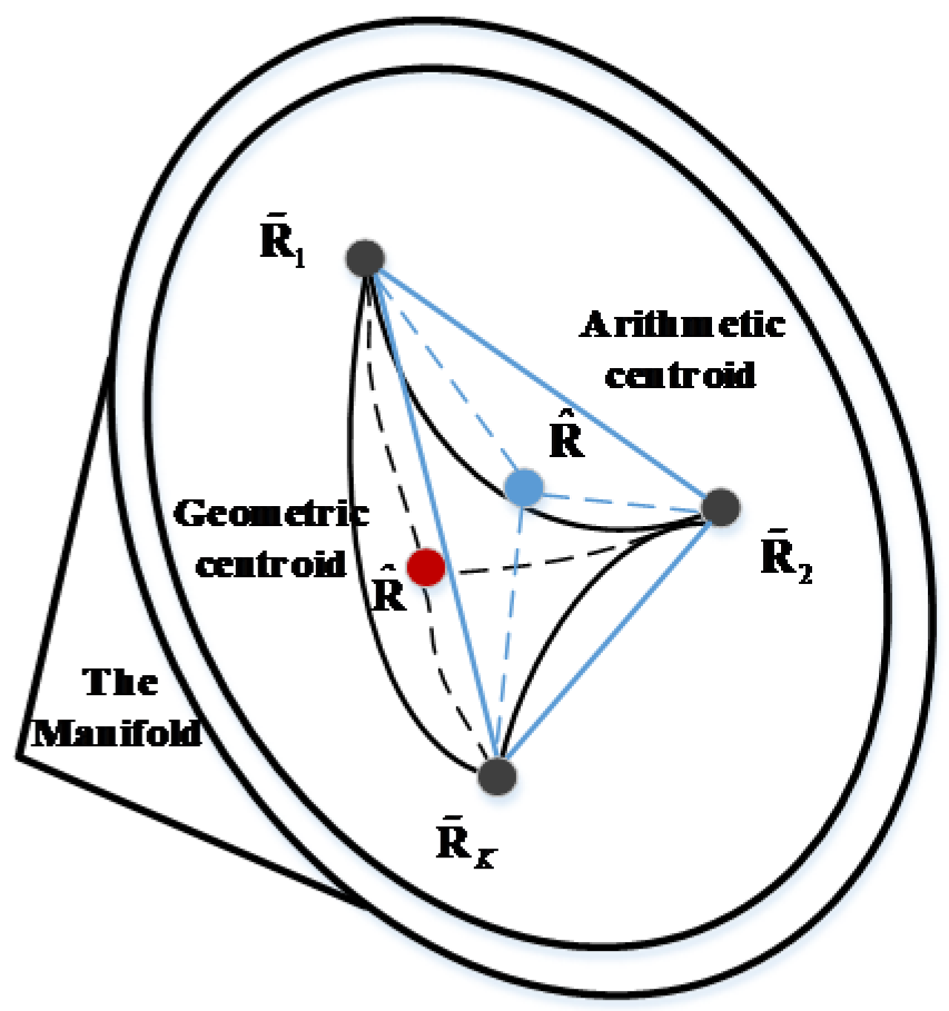
When , the matrix is the geometric median; and , is the geometric mean. Herein, we dub the
centroid of points along the manifold surface as the geometric centroid and the
centroid of points along with the straight-line distance as the arithmetic
centroid. For a more intuitive illustration, the difference between the
geometric centroid and the arithmetic centroid is illustrated in Figure 4.

Figure 4.
The difference between the geometric centroid and arithmetic centroid.
The dissimilarity metric can directly be the distance in (12), however, it
is not an easy task to derive closed-form expressions for the distance (at
least to the best of the authors’ knowledge). Therefore, the crucial question
of how to measure the distance and dissimilarity of different points on
manifolds efficiently must be addressed. A natural choice for the dissimilarity
metric to solve (15) is the affine invariant Riemannian metric
where is the eigenvalue of . This metric is an important dissimilarity metric but is computationally cumbersome [36]. Due to the complexity of STAP, the Riemannian metric is inappropriate, and it is imperative to have a good metric for approximating distances on generalized surfaces. The approximating metric directly affects the extraction and utilization of the structure of the data; thus, different scenarios may have a different optimal metric. For example, maximizing the discriminative features between the target and background is the key point for target detection, while for background estimation, it is important to extract the common features from the contaminated data. Therefore, it is necessary to combine this with practical application to obtain appropriate dissimilarity metrics.
4.2. Criteria for Dissimilarity Metric on Manifolds
Four typical types of dissimilarity metrics: the arithmetic, Riemannian distance, Kullback–Leibler, and total skew Jensen divergence [37] (TSJD, belonging to Bregman divergences [38]) are considered to obtain an appropriate metric for our problem. Based on these metrics, we investigate which criterion should be used to decide which metric to exploit in our scenario. First, precise estimation with small sample support is required in heterogeneous environments due to the limited homogeneous samples. Second, it is important for our method to be statistically robust to outliers. Third, a huge amount of computation is a tricky issue with large array elements. Therefore, combining these practical needs, good dissimilarity metrics should be precise with small sample support, be robust, and have a low complexity. Namely, the IF, robustness to corrupted training data, and computational efficiency are proposed as the criteria to evaluate the different dissimilarity metrics.
As stated before, Euclidean tools are not adapted for HPD matrices. The distance between and in (16) is employed to assess the property of robustness, where and represent the estimated CCM with and without outliers in the training data, respectively. Since the estimated matrix may have no explicit closed-form expression under the aforementioned dissimilarity metrics herein, we try to conduct a quantitative comparison of IF and robustness properties in the simulated experiment. A standard STAP system that employs 8 array elements and 10 pulses is considered. Assume that the clutter data obey the K distribution, and the clutter to noise ratio is set to 40 dB. As we are interested in heterogeneous environments, the IF and robustness performance are discussed under the condition of small sample support in the simulation. Therefore, the number of training data is set to 32, and an outlier is located at the range bin when considering the property of
robustness. This means that, according to (6) and (16), the IF and the distance
between and can be calculated. Meanwhile, for the computational cost, if the metric has a closed-form, it will be regarded as having low complexity. Then, the properties of the aforementioned metrics are summarized in Table 1.

Table 1.
Properties of the aforementioned metrics.
Table 1 indicates that the arithmetic method has a relatively poor IF and statistical robustness performance in small sample support. KL is a good way to measure the dissimilarity due to its low complexity; however, it is easily biased by the chosen coordinate and has a poor IF performance. The TSJD provides the desired invariance to coordinate, is robust, has a relatively high IF, and has a low computational cost compared with the Riemannian metric. Therefore, TSJD is selected as the dissimilarity metric.
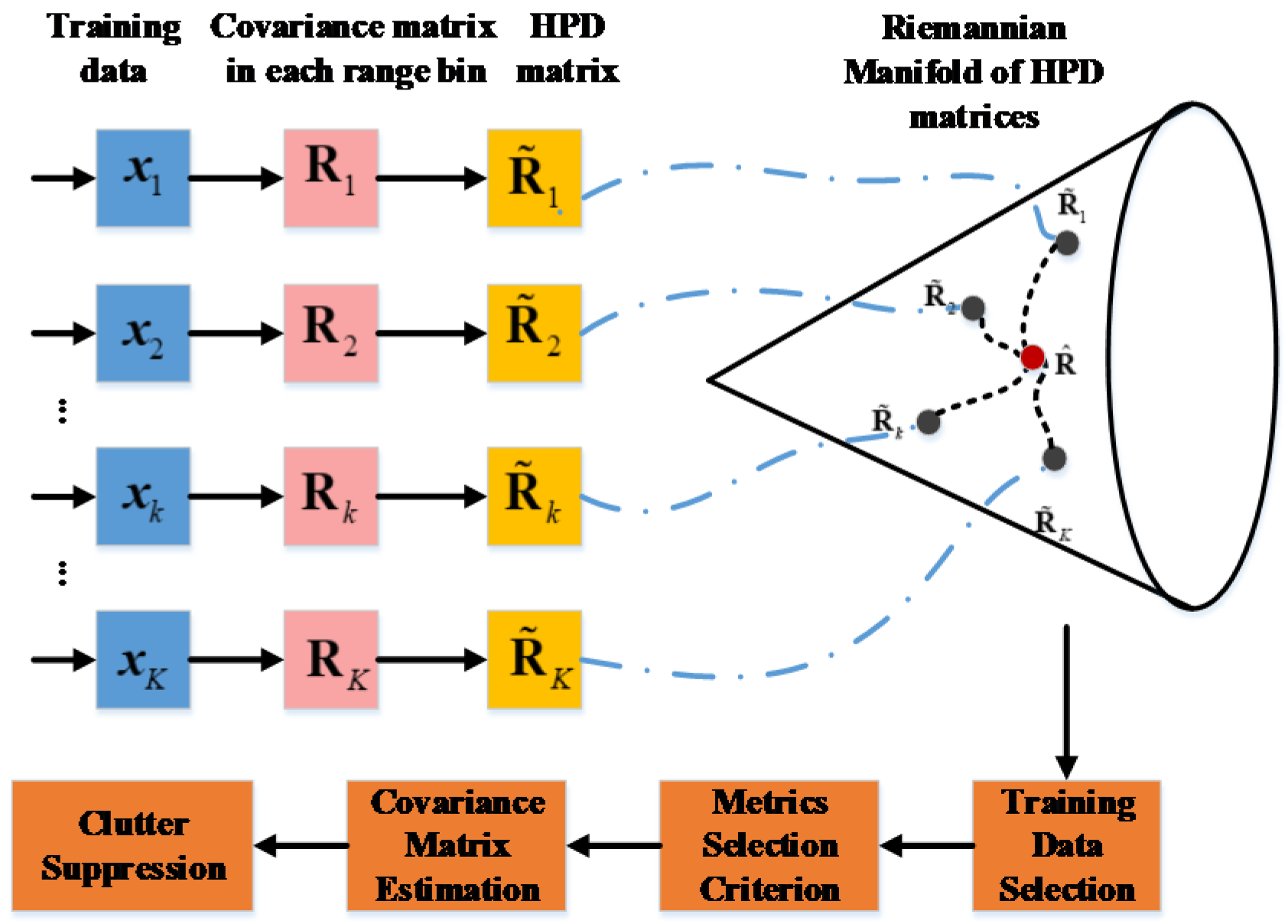
To summarize, a specific scheme for the clutter suppression on manifolds is shown in Figure 5. The process of constructing the covariance matrix of the sample from a single sample itself has the ability to reduce the number of samples required. However, the reduction in the number of samples required in the proposed method is not only produced by the covariance matrix construction of the received data but is also related to the data structure on manifolds. A detailed simulation will be conducted in the subsequent simulation.

Figure 5.
Scheme of the proposed method with application to STAP.
As observed in Figure 5, the CCM is constructed using the received data in each bin first. Based on the CCM, the manifold is established, and then homogeneous samples are selected according to a binary hypothesis test. Afterward, the TSJD is exploited as the geometric dissimilarity metric. Thus, the iteration of the estimated CCM is
where represents the skew factor, and represents the updated renormalized weights at stage is given by
and denotes the loss function. is the differential of . Generally, the square loss function, logarithms,
and exponentials are the typical loss functions. Among them, the square loss
function is the maximum likelihood estimation of parameters. Moreover, the
logarithms and exponentials are sensitive to noise when compared with the
square loss function. Therefore, in this paper, we choose the square loss
function, namely, . Once the CCM is obtained, the adaptive weights for clutter
suppression are calculated by (7).
5. Experimental Results and Analysis
In this section, experiments on simulated and real data demonstrate the performance of the proposed method. Both competing conventional methods in Euclidean space and other geometric methods based on manifolds are discussed. We denote the arithmetic mean performed on the covariance matrix construction in (9) as the arithmetic method. Then, the LSMI, 3DT, arithmetic, EASTR [18], random matrix improved (RMI) [30], Karcher [32], and m-estimators [39] are compared to illustrate the potential of the proposed method. To compare under fair conditions, the initialization matrix of the methods that need iteration is set to be the identity matrix.
5.1. Clutter Suppression and Target Detection Performance
5.1.1. Simulated Data
First, experiments conducted on the simulated data are shown. The main radar parameters of the simulation are listed in Table 2. The Monte Carlo technique is exploited to test the performance and 500 independent Monte Carlo trials are run.

Table 2.
The parameters for simulation.
For the training data selection experiment, the range bin is assumed to be the CUT, and the data in set are homogenous samples with CUT, which obey a K
distribution. Meanwhile, the data in the set are heterogeneous samples, which obey a normal
distribution. Herein, the CUT is target free and the CCM of CUT can be viewed
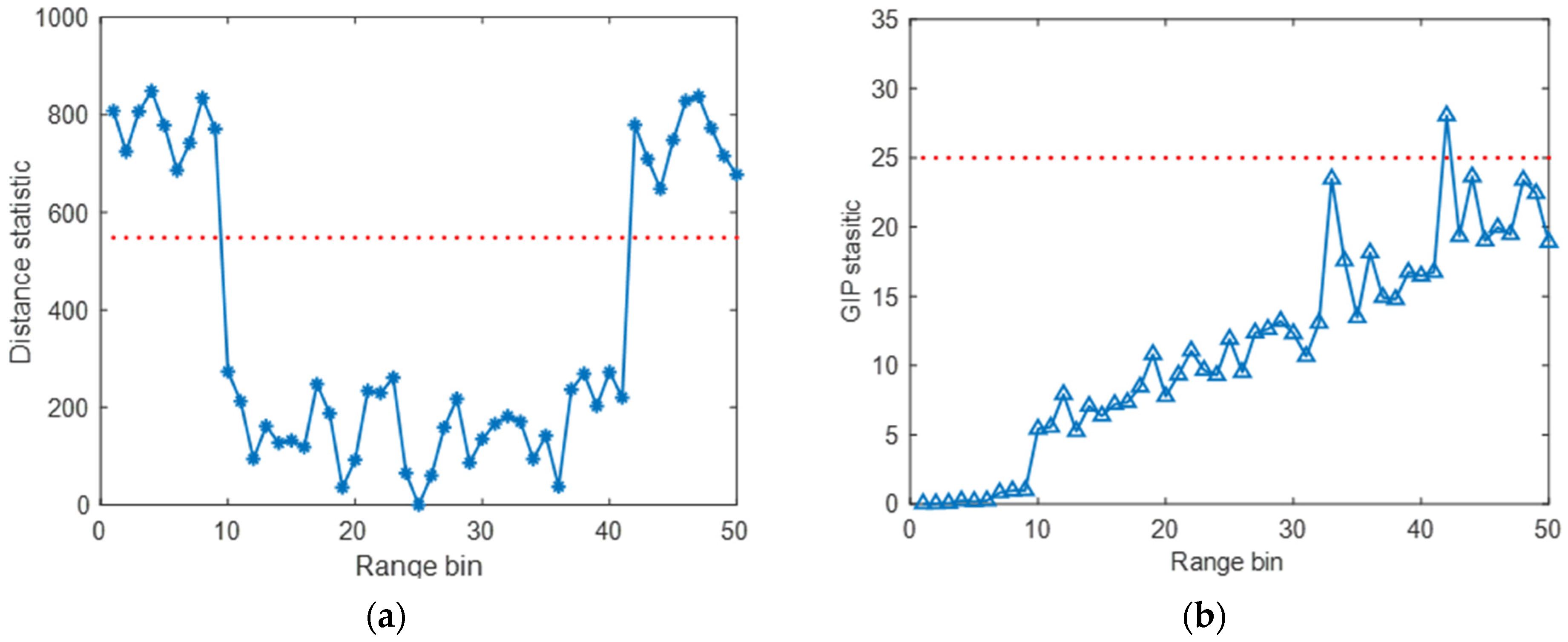
as . The probability of classifying data as heterogeneous when they are homogeneous is set to be . Using the probability , the threshold is obtained. The comparison result of homogeneous training data selection is shown in Figure 6. It is seen that the homogeneous samples can be selected effectively by the proposed method. Meanwhile, since the heterogeneous training data with CUT are the data that obey different distributions, rather than the data with different power, the GIP test fails to obtain a satisfactory performance.
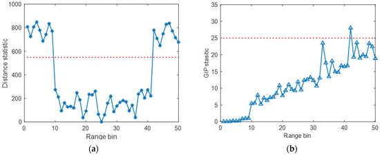
Figure 6.
The result of homogeneous training data selection; (a) the proposed method; (b) the GIP test.
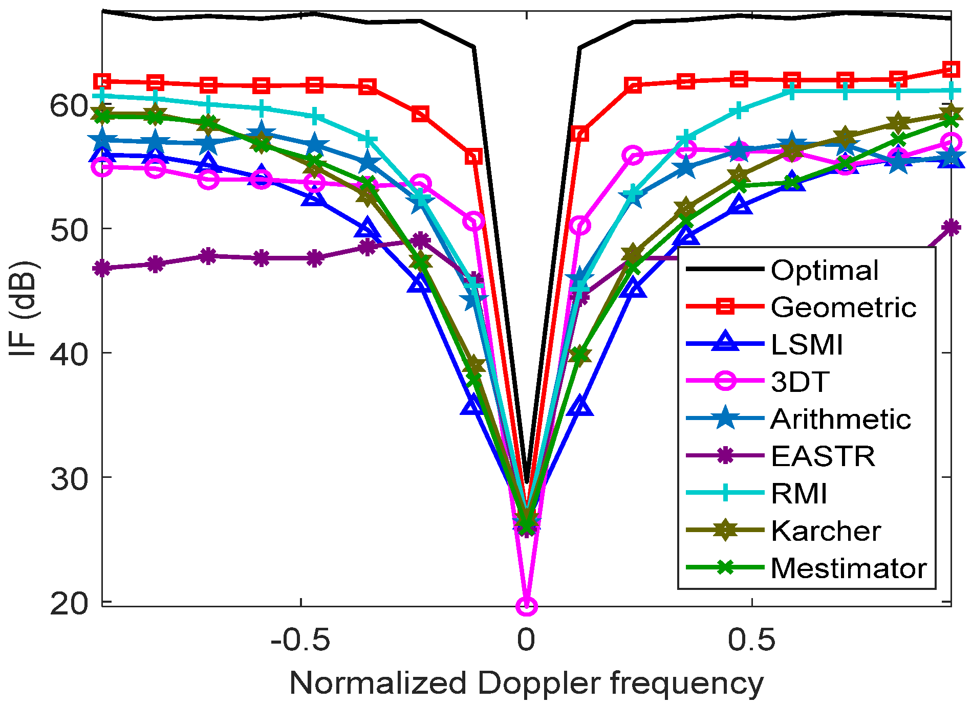
With the selected training data (the number of homogeneous samples in is 32), the IF performance of different methods in limited samples is depicted in Figure 7. The higher IF is, the larger the output SCNR is, and the wider the notch result, the poorer the low Doppler shift signal detection. As seen in Figure 7, with small sample support, the IF of the proposed method (dubbed as the geometric method) has a higher gain and sharp notch and is greatly improved compared with the typical methods in Euclidean space (the LSMI, 3DT, and EASTR method). Furthermore, the other geometric methods (the Karcher, m-estimator, and RMI method) are generally better than typical methods in Euclidean space.
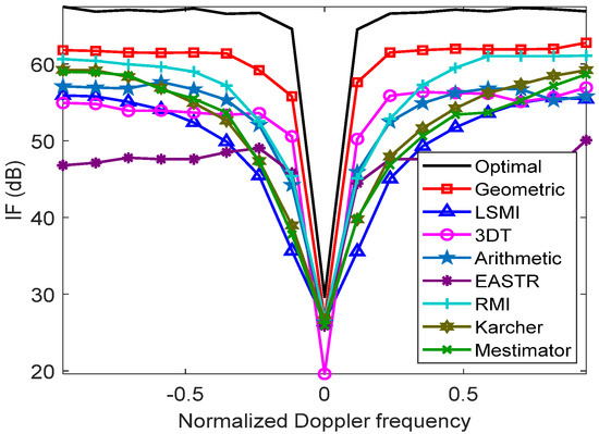
Figure 7.
Improvement factor (IF) performance.
To illustrate the impact of homogeneous training data on the proposed method, the output SCNR concerning the number of training data is provided in Figure 8. The comparison results indicate that the EASTR method has an unsatisfactory performance with limited training data. In addition, when the number of samples is less than 60, the proposed method is better than other methods. Afterward, with the increase in samples, the performance of each method gradually approaches. The SCNR of the arithmetic method is always 2 dB lower than that of the proposed method. The reason fewer training samples are needed for the proposed method is due to the geometric metric on manifolds. This is because different elements of the CCM play different roles in the clutter matrix estimation, and the main diagonal occupies a more important position. When we use the Frobenius norm in the Euclidean space to measure the dissimilarity, each element is treated equally. However, with the geometric metrics on manifolds, this is equivalent to exploiting embedding mapping (similar to weighted, but not linear) with different elements, indicating that different elements couple together and play different roles in the estimation. We can take the Riemannian metric as an example to illustrate this further. Denote a set of HPD matrices and compute all the pairwise distances
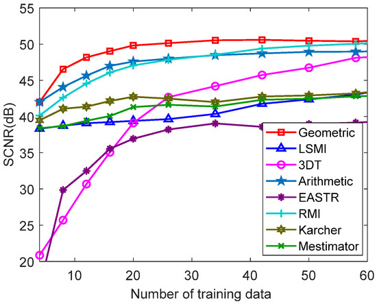
Figure 8.
Output SCNR against the number of training data.
The matrices , are coupled together. If we rearrange the elements of the matrices, the distances will be different. Hence, in the case of small sample support, the metric on manifolds allows us to obtain a more accurate CCM by embedding mapping. Then, under the same conditions, the number of samples required for the estimation on manifolds can be lower. This verifies that the superior performance of the proposed method is not only produced by the construction of CCM in (9), but also the geometric metric on manifolds.
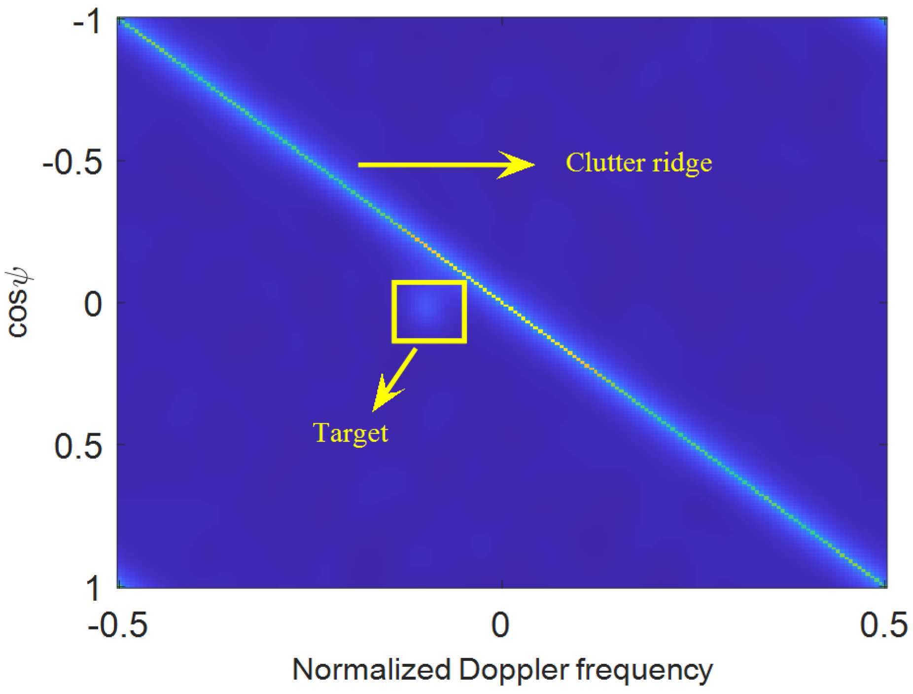
In addition to the clutter suppression performance, the moving target detection performance is also discussed. We assume there to be a weak target in strong clutter environments, and that the presumed target is located at the range bin with a velocity of 4.27 m/s and a
spatial angle of 89°. The spatiotemporal spectrum is depicted in Figure 9. The detection probability performances
of adaptive matched filter (AMF) detectors in limited samples are evaluated via
the Monte Carlo technique. The threshold value in the AMF detector is set
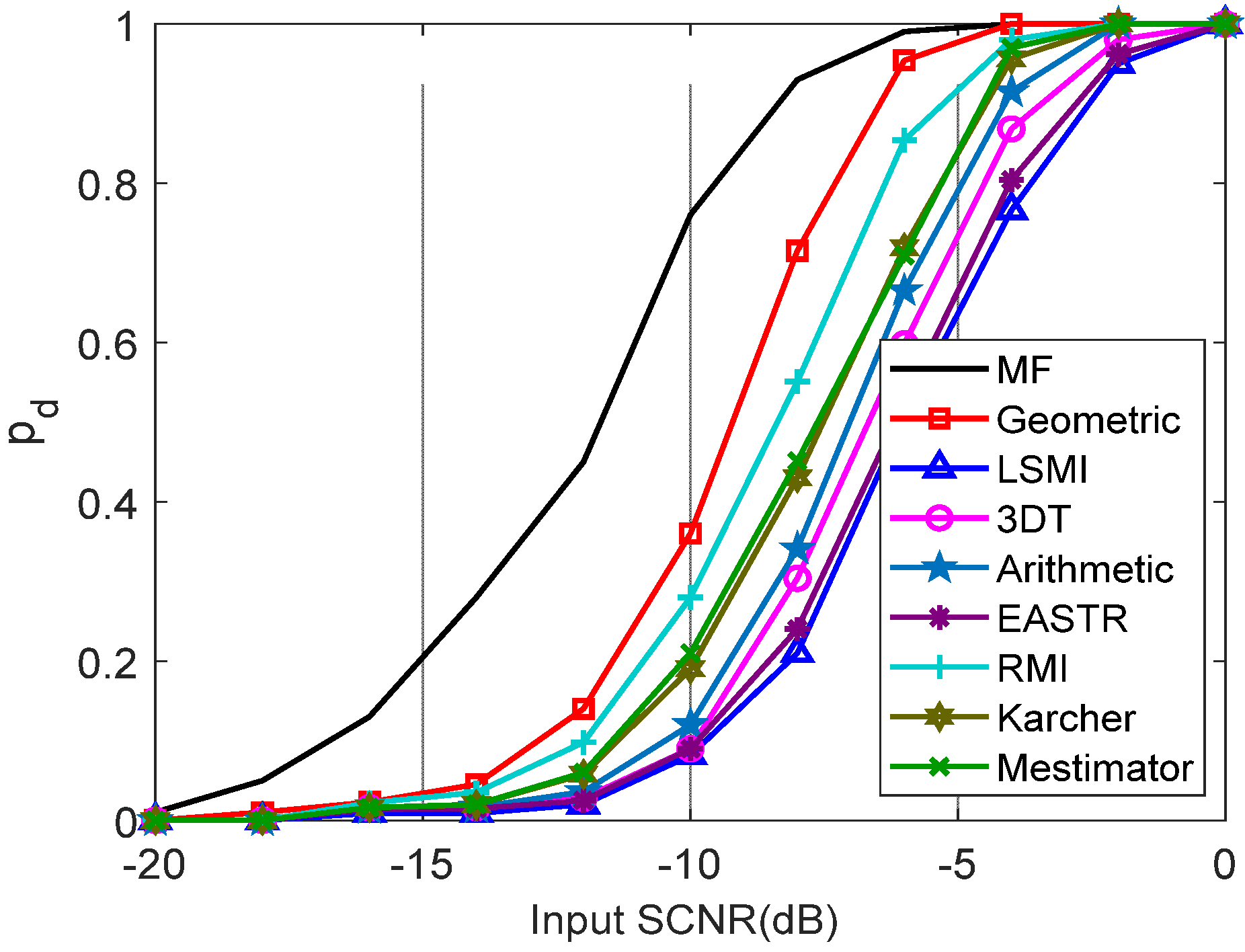
according to [40]. Figure 10 provides the detection probability with respect to input SCNR, where , and the input SCNR varies from −20 to 0 dB. As observed, Figure 10 demonstrates that the proposed method achieves better performance than others.
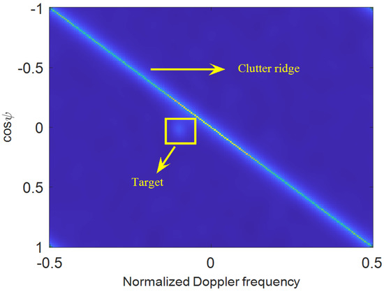
Figure 9.
Spatiotemporal spectrum.
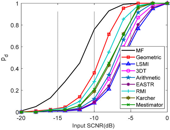
Figure 10.
The detection probability with respect to input SCNR.
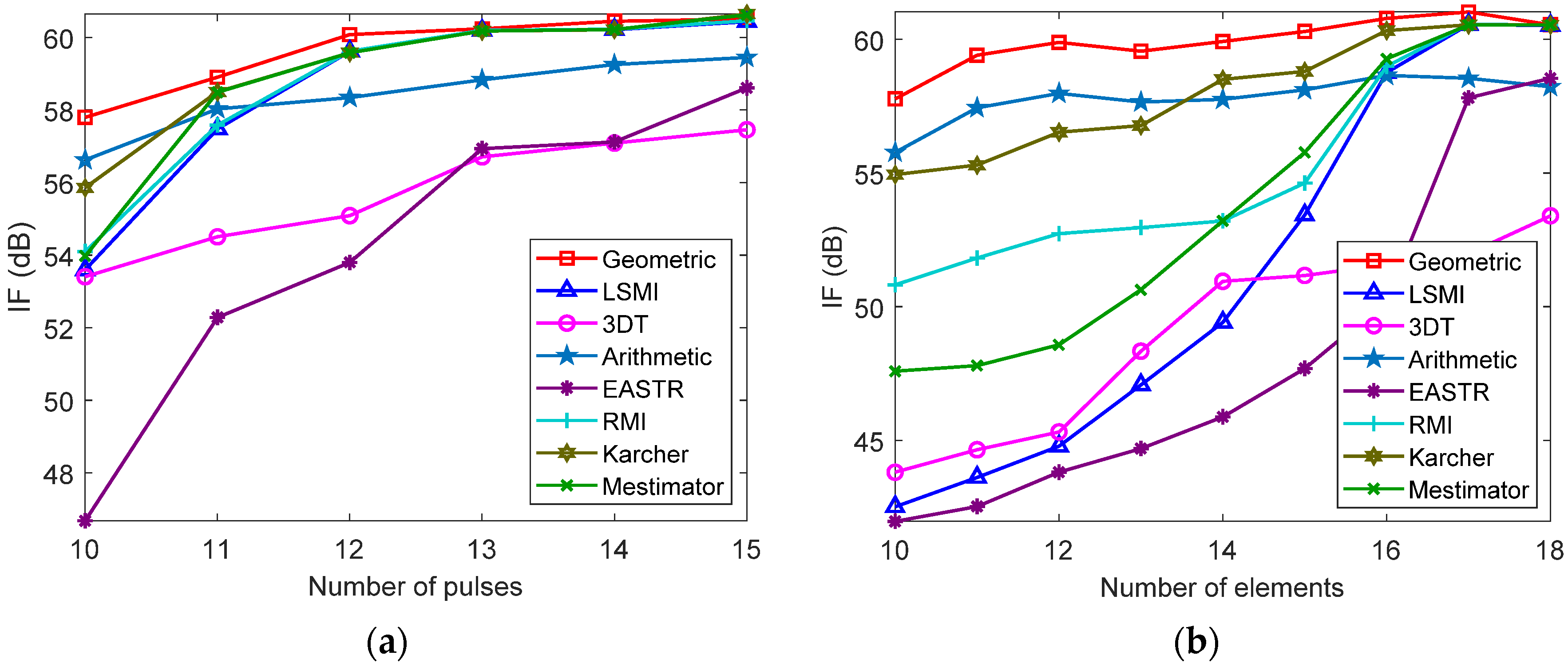
The influences of the number of pulses and array elements on the performances for different methods are depicted in Figure 11a,b, respectively. As observed, the IF of the proposed method is better than the others at first. Afterward, as the number of array elements and pulses increases, the IF of all methods tends to be consistent.
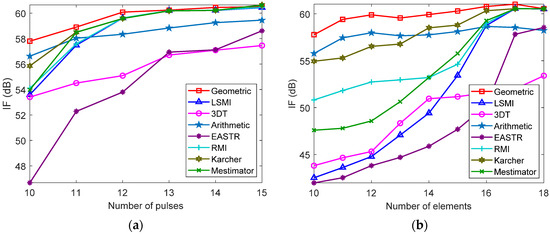
Figure 11.
The influence of the DoF on the IF performance: (a) the influence of the number of pulses; (b) the influence of the number of elements.
5.1.2. Real Data
To further demonstrate the effectiveness of the proposed method, experiments are performed on the real data file t38pre01v1.mat in the Mountain-Top data set [41,42]. There are 14 antenna elements, 16 coherent pulses, and 403 range bins. A target is located in the range bin with a normalized Doppler frequency of
0.25 and a spatial angle of −15°. Considering the limited samples scenario, we
use the data from 114 to 172 range bins as dataset 1. As the data are
relatively homogeneous, three outliers are added to the range bins from 114 to
116 to demonstrate our proposed method. Therefore, the data in the set are the homogenous samples, correspondingly, the
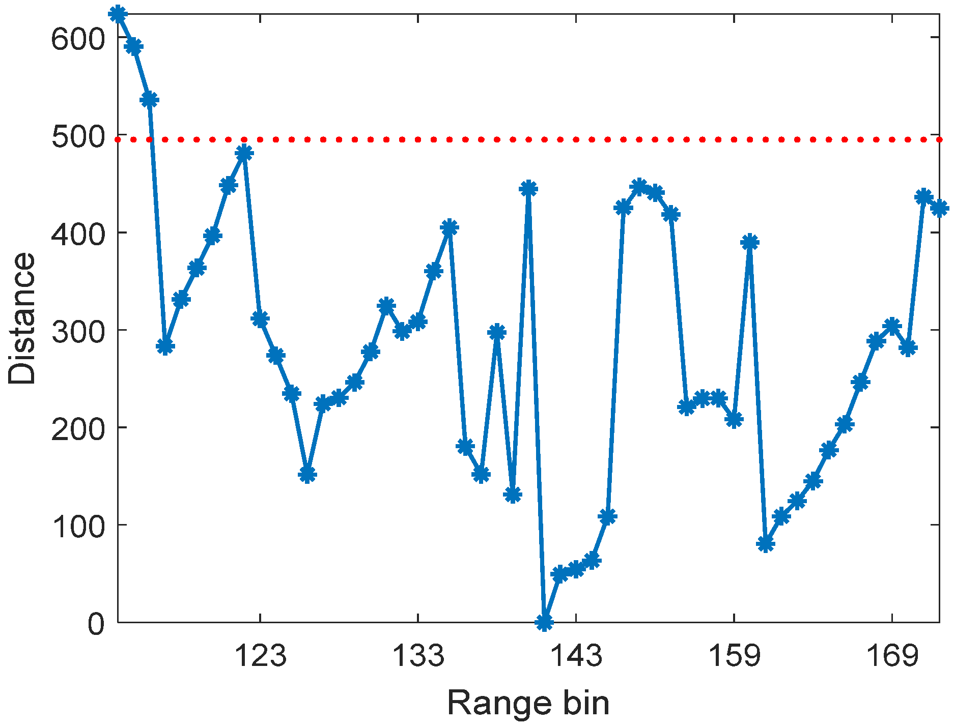
data in the set are heterogeneous samples. The result of the
homogeneous training data selection is shown in Figure 12. As observed, the outliers can be selected due to their large
distance. Figure 13 illustrates the
output power of different methods after applying the space-time adaptive
filter. This indicates that all the algorithms can detect the target effectively.
However, the clutter residual at the other range bins for the proposed method
is weaker than the others.

Figure 12.
The result of homogeneous training data selection.
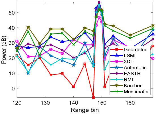
Figure 13.
The output power of different methods.
To sufficiently demonstrate the improvement produced by the proposed method in the case of limited samples, the data with a presumed target are used as dataset 2. In dataset 2, the presumed target is injected in the range bin, and the data of range bins 66 to 118 are exploited as training samples. The normalized Doppler frequency and spatial angle of the target are also set to 0.25 and −15°, respectively. To perform a quantitative comparison, the averaged output SCNR of the selected range bins (excluding eight range bins around the target) is calculated, where the output SCNR denotes the ratio of the target output power to the averaged output power of selected range bins. Specific values are reported in Table 3. The results achieved with real data are consistent with those achieved with simulated data.

Table 3.
The output SCNR.
5.2. Influence Analysis of Outliers
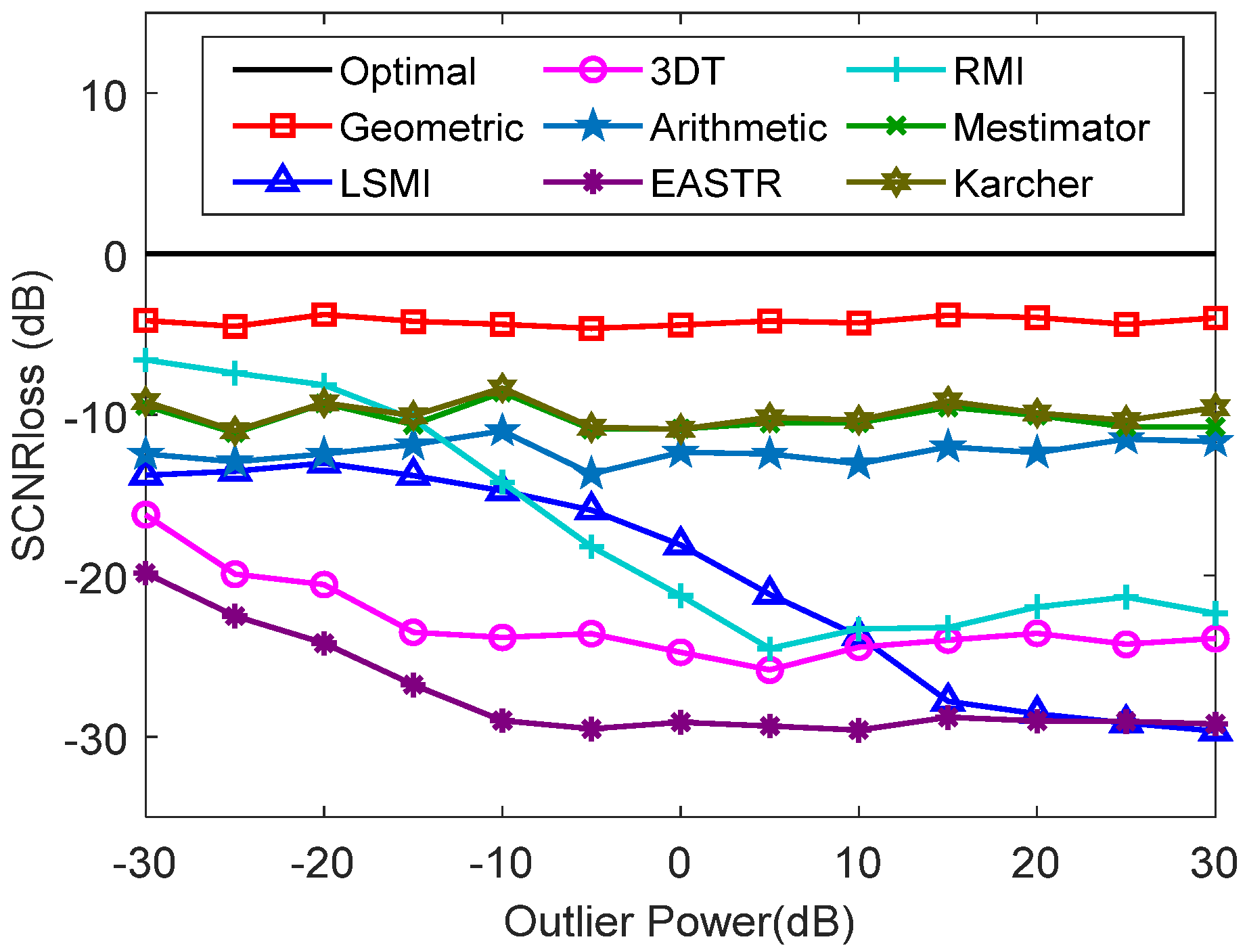
Based on the previous subsection, the proposed method appears to be suitable for situations with limited samples. Generally, if there are contaminated training data, the clutter suppression performance will be greatly degraded. Therefore, to illustrate the impact of outliers, the simulation with outliers is performed using different methods. We assumed that the main parameters are consistent with those in Table 2. The training data number is set to be 32, and there are two outliers with high power in the training data. The normalized Doppler frequency and the azimuth of outliers are −0.3 and 90°, respectively. We evaluate the performance by comparing the SCNR loss (), which is defined by
The against the power with two outliers in the training data is shown in Figure 14. As observed, the of the LSMI, 3DT, EASTR, and RMI methods is clearly increased in the presence of outliers, while the of the arithmetic, Karcher, m-estimator, and the proposed method is almost unchanged. Compared with the case without outliers, the influence of the arithmetic, Karcher, m-estimator, and the proposed method is less than 0.5 dB, whereas that of RMI method is about 15dB. Hence, the RMI method is easily affected by outliers. Figure 15 is presented to help assess the against the number of outliers. The proposed method achieves better performance when the number of outliers increases slightly. The proposed method is superior to the other methods in the presence of outliers. The reason for this can be deduced by the influence function. If there are outliers, , in the training data, the influence function of the metric of the proposed method (TSJD) can be calculated by
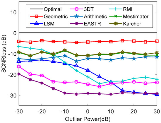
Figure 14.
The SCNR loss against the power with 2 outliers.
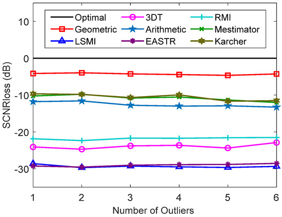
Figure 15.
The SCNR loss against the number of outliers.
Denote ,, then, the influence function can be reformulated by
When , and , is bounded, the influence function satisfies
where is a constant. Hence, the dissimilarity metric is robust to outliers, which allows for its robust performance in heterogeneous environments.
6. Conclusions
This paper focuses on a heterogeneous clutter suppression problem for an airborne radar system. The training data are characterized on the Riemannian manifold of HPD matrices. Then, it is revealed that the training data with different distributions with the same power are separated, while those with the same distribution are close. With these properties, the heterogeneous samples can be eliminated. After that, combining these practical needs, an improved clutter suppression method based on manifolds is proposed with the selected limited samples. The results show that by taking advantage of the geometric dissimilarity on manifolds, the requirement for training samples for clutter suppression can be reduced. Afterward, the performances of clutter suppression, target detection, and the influences of outliers (discrete clutter) are investigated to evaluate the potential of the proposed method. The experiments show that the proposed method is not only competitive in the case of limited samples but also has a good robustness to discrete clutter. In possible future research, it is worth studying the geometric metric optimization on manifolds. Additional research direction may concern the fast algorithm for geometric barycenter to estimate covariance matrix.
Author Contributions
Writing—original draft preparation, X.C.; writing—review and editing, X.C., Y.C., H.W. (Hao Wu) and H.W. (Hongqiang Wang); supervision, H.W. (Hongqiang Wang); conceptualization and methodology, X.C.; investigation, Y.C.; resources and software, H.W. (Hao Wu). All authors have read and agreed to the published version of the manuscript.
Funding
This research was funded by the National Natural Science Foundation of China under grant no. 61871472.
Institutional Review Board Statement
Not applicable.
Informed Consent Statement
Not applicable.
Data Availability Statement
The data presented in this study are available at http://spib.rice.edu/spib/mtn_top.html. (accessed on 29 May 2021).
Conflicts of Interest
The authors declare no conflict of interest.
References
- Huang, S.; Liu, Y.; He, Y.; Zhang, T.; Peng, Z. Structure-adaptive clutter suppression for infrared small target detection: Chain-growth filtering. Remote Sens. 2019, 12, 47. [Google Scholar] [CrossRef]
- Gracheva, V.; Ender, J. Multichannel analysis and suppression of sea clutter for airborne microwave radar systems. IEEE Trans. Geosci. Remote Sens. 2016, 54, 2385–2399. [Google Scholar] [CrossRef]
- Guo, Y.; Liao, G.; Li, J.; Gu, T. A clutter suppression method based on NSS-RPCA in heterogeneous environments for SAR-GMTI. IEEE Trans. Geosci. Remote Sens. 2020, 58, 5880–5891. [Google Scholar] [CrossRef]
- Lightstone, L.; Faubert, D.; Rempel, G. Multiple phase centre DPCA for airborne radar. In Proceedings of the IEEE National Radar Conference, Los Angeles, CA, USA, 12–13 March 1991; pp. 36–40. [Google Scholar]
- Chapin, E.; Chen, C.W. Airborne along-track interferometry for GMTI. IEEE Aerosp. Electron. Syst. Mag. 2009, 24, 13–18. [Google Scholar] [CrossRef]
- Ward, J. Space-Time Adaptive Processing for Airborne Radar; Technical Report TR-1015; MIT Lincoln Laboratory: Lexington, MA, USA, 1994. [Google Scholar]
- Melvin, W. Space-time adaptive radar performance in heterogeneous clutter. IEEE Trans. Aerosp. Electron. Syst. 2000, 36, 621–633. [Google Scholar] [CrossRef]
- Klemm, R. Principles of Space-Time Adaptive Processing, 3rd ed.; Radar, Sonar, Navigation and Avionics Series; IET: London, UK, 2006. [Google Scholar]
- Guerci, J.R. Space-Time Adaptive Processing for Radar; Artech House: Norwood, MA, USA, 2003. [Google Scholar]
- Reed, I.; Mallett, J.; Brennan, L. Rapid convergence rate in adaptive arrays. IEEE Trans. Aerosp. Electron. Syst. 1974, AES-10, 853–863. [Google Scholar] [CrossRef]
- Martorella, M.; Gelli, S.; Bacci, A. Ground moving target imaging via SDAP-ISAR processing: Review and new trends. Sensors 2021, 21, 2391. [Google Scholar] [CrossRef]
- Rangaswamy, M.; Michels, J.H.; Himed, B. Statistical analysis of the non-homogeneity detector for STAP applications. Digit. Signal Process. 2004, 14, 253–267. [Google Scholar] [CrossRef]
- Shackelford, A.; Gerlach, K.; Blunt, S. Partially adaptive STAP using the FRACTA algorithm. IEEE Trans. Aerosp. Electron. Syst. 2009, 45, 58–69. [Google Scholar] [CrossRef]
- Tang, B.; Tang, J.; Peng, Y. Detection of heterogeneous samples based on loaded generalized inner product method. Digit. Signal Process. 2012, 22, 605–613. [Google Scholar] [CrossRef]
- Li, X.; Xie, W.; Wang, Y. Cyclic training sample selection and cancellation technique for airborne STAP radar under nonhomogeneous environment. Digit. Signal Process. 2020, 104, 102803. [Google Scholar] [CrossRef]
- Song, C.; Wang, B.; Xiang, M.; Wang, Z.; Xu, W.; Sun, X. A novel post-doppler parametric adaptive matched filter for airborne multichannel radar. Remote Sens. 2020, 12, 4017. [Google Scholar] [CrossRef]
- Zhang, L.; Bao, Z.; Liao, G. A study of reduced-rank stap. J. Electron. (China) 2000, 17, 289–296. [Google Scholar] [CrossRef]
- Kang, B. Estimation of structured covariance matrices for radar STAP. IEEE Trans. Aerosp. Electron. Syst. 2015, 30, 24–25. [Google Scholar] [CrossRef]
- Guo, L.; Deng, W.; Yao, D.; Yang, Q.; Ye, L.; Zhang, X. A knowledge-based auxiliary channel STAP for target detection in shipborne HFSWR. Remote Sens. 2021, 13, 621. [Google Scholar] [CrossRef]
- Burintramart, S.; Sarkar, T.K.; Zhang, Y.; Wicks, M.C. Performance comparison between statistical-based and direct data domain STAPs. Digit. Signal Process. 2007, 17, 737–755. [Google Scholar] [CrossRef]
- Wang, P.; Wang, Z.; Li, H.; Himed, B. Knowledge-aided parametric adaptive matched filter with automatic combining for covariance estimation. IEEE Trans. Signal Process. 2014, 62, 4713–4722. [Google Scholar] [CrossRef]
- Han, S.; Fan, C.; Huang, X. A novel STAP based on spectrum-aided reduced-dimension clutter sparse recovery. IEEE Geosci. Remote Sens. Lett. 2017, 14, 213–217. [Google Scholar] [CrossRef]
- Hua, X.; Ono, Y.; Peng, L.; Cheng, Y.; Wang, H. Target detection within nonhomogeneous clutter via total bregman divergence-based matrix information geometry detectors. IEEE Trans. Signal Process. 2021. [Google Scholar] [CrossRef]
- Arnaudon, M.; Barbaresco, F.; Yang, L. Riemannian medians and means with applications to radar signal processing. IEEE J. Sel. Top. Signal Process. 2013, 7, 595–604. [Google Scholar] [CrossRef]
- Barbaresco, F. Innovative tools for radar signal processing Based on Cartan’s geometry of SPD matrices & Information Geometry. In Proceedings of the 2008 IEEE Radar Conference, Rome, Italy, 26–30 May 2008; pp. 1–6. [Google Scholar]
- Abramovich, Y.I.; Besson, O. Regularized covariance matrix estimation in complex elliptically symmetric distributions using the expected likelihood approach—Part 1: The over-sampled case. IEEE Trans. Signal Process. 2013, 61, 5807–5818. [Google Scholar] [CrossRef]
- Besson, O.; Abramovich, Y.I. Regularized covariance matrix estimation in complex elliptically symmetric distributions using the expected likelihood approach—Part 2: The under-sampled case. IEEE Trans. Signal Process. 2013, 61, 5819–5829. [Google Scholar] [CrossRef][Green Version]
- Hua, X.; Peng, L. MIG median detectors with manifold filter. Signal Process. 2021, 188, 108176. [Google Scholar] [CrossRef]
- Dong, G.; Kuang, G. Target recognition in SAR images via classification on riemannian manifolds. IEEE Geosci. Remote Sens. Lett. 2014, 12, 199–203. [Google Scholar] [CrossRef]
- Tiomoko, M.; Bouchard, F.; Ginolhac, G.; Couillet, R. Random matrix improved covariance estimation for a large class of metrics. J. Stat. Mech. Theory Exp. 2020, 2020, 124011. [Google Scholar] [CrossRef]
- Aubry, A.; De Maio, A.; Pallotta, L.; Farina, A. Covariance matrix estimation via geometric barycenters and its application to radar training data selection. IET Radar Sonar Navig. 2013, 7, 600–614. [Google Scholar] [CrossRef]
- Balaji, B.; Barbaresco, F. Application of riemannian mean of covariance matrices to space-time adaptive processing. In Proceedings of the 2012 9th European Radar Conference, Amsterdam, The Netherlands, 31 October–2 November 2012; pp. 50–53. [Google Scholar]
- Moakher, M. A differential geometric approach to the geometric mean of symmetric positive-definite matrices. SIAM J. Matrix Anal. Appl. 2005, 26, 735–747. [Google Scholar] [CrossRef]
- Harandi, M.; Salzmann, M.; Hartley, R. Dimensionality reduction on spd manifolds: The emergence of geometry-aware methods. IEEE Trans. Pattern Anal. Mach. Intell. 2018, 40, 48–62. [Google Scholar] [CrossRef]
- van der Maaten, L.; Hinton, G. Visualizing data using T-SNE. J. Mach. Learn. Res. 2008, 9, 2579–2605. [Google Scholar]
- Amari, S. Information Geometry and Its Applications; Springer: Tokyo, Japan, 2016. [Google Scholar]
- Nielsen, F.; Nock, R. Total jensen divergences: Definition, properties and clustering. In Proceedings of the 2015 IEEE International Conference on Acoustics, Speech and Signal Processing (ICASSP), South Brisbane, QLD, Australia, 19–24 April 2015; pp. 1–27. [Google Scholar]
- Nielsen, F.; Nock, R. Sided and symmetrized bregman centroids. IEEE Trans. Inf. Theory 2009, 55, 2882–2904. [Google Scholar] [CrossRef]
- Ilea, I.; Bombrun, L.; Terebes, R.; Borda, M.; Germain, C. An m-estimator for robust centroid estimation on the manifold of covariance matrices. IEEE Signal Process. Lett. 2016, 23, 1255–1259. [Google Scholar] [CrossRef]
- Robey, F.; Fuhrmann, D.; Kelly, E.; Nitzberg, R. A CFAR adaptive matched filter detector. IEEE Trans. Aerosp. Electron. Syst. 1992, 28, 208–216. [Google Scholar] [CrossRef]
- Available online: http://spib.rice.edu/spib/mtn_top.html (accessed on 29 May 2021).
- Titi, G.; Marshall, D. The ARPA/NAVY mountaintop program: Adaptive signal processing for airborne early warning radar. In Proceedings of the 1996 IEEE International Conference on Acoustics, Speech, and Signal Processing Conference Proceedings, Atlanta, GA, USA, 9 May 1996; pp. 1165–1168. [Google Scholar]
Publisher’s Note: MDPI stays neutral with regard to jurisdictional claims in published maps and institutional affiliations. |
© 2021 by the authors. Licensee MDPI, Basel, Switzerland. This article is an open access article distributed under the terms and conditions of the Creative Commons Attribution (CC BY) license (https://creativecommons.org/licenses/by/4.0/).

