Abstract
Obtaining water body images quickly and reliably is important to guide human production activities and study urban change. This paper presents a fast and accurate method to identify water bodies in complex environments based on UAV high-resolution images. First, an improved U-Net (SU-Net) model is proposed in this paper. By increasing the number of connections in the middle layer of the neural network, more image features can be retained through S-shaped circular connections. Second, aiming at the interference of mixed ground objects and dark ground objects on water detection, the fusion of a deep learning network and visual features is investigated. We analyse the influence of a wavelet transform and grey level cooccurrence matrix (GLCM) on water extraction. Using a confusion matrix to evaluate accuracy, the following conclusions are drawn: (1) Compared with existing methods, the SU-Net method achieves a significant improvement in accuracy, and the overall accuracy (OA) is 96.25%. The kappa coefficient (KC) is 0.952. (2) SU-Net combined with the GLCM has a higher accuracy (OA is 97.4%) and robustness in distinguishing mixed and dark objects. Based on this method, a distinct water boundary in urban areas, which provides data for urban water vector mapping, can be obtained.
1. Introduction
Urban water bodies are an important part of maintaining urban ecological balance. Economical and rapid access to urban surface water bodies has an important role in ecological environmental assessments, water resource management, policy implementation and management decision-making [1,2].
Remote sensing is a powerful tool for quickly obtaining image data [3]. Optical satellite remote sensing can provide long-term and large-area true colour images, through which visual interpretations and automatic classification can be carried out. As basic information to obtain the locations of water areas, remote sensing images have been widely employed in many fields. These applications include remote sensing based on IKONOS panchromatic image extraction of high-precision urban water areas [4], high-resolution remote sensing images obtained from Gaofen-1 and Ziyuan-3 for aquaculture water extraction [5], the application of WorldView-2 panchromatic and multispectral image data from Antarctic coastal water extraction [6], and the application of Landsat in large area and long-time series water research [7,8]. However, many clouds are usually present during emergencies and other special events, which limits the use of optical satellite images to a certain extent. Because of its ability to penetrate clouds and fog, spaceborne radar can collect data without being affected by weather conditions, which makes it an effective alternative method for water extraction [9,10,11], for dynamic monitoring of river basin water bodies [12], for the detection of water bodies in urban environments [13] and for monitoring urban flood areas [14,15,16]. However, it has been indicated that satellite remote sensing can be effectively used for water body extraction [17,18]. There are still many shortcomings in urban water body mapping, such as the low real time data collection and processing caused by the long revisit cycle time, low-quality images caused by cloud cover in rainy weather and the weak ability to extract small bodies of water (small ponds and narrow rivers) due to the limited spatial resolution of most satellite remote sensing [19] Aerial remote sensing can overcome these limitations and is an ideal tool for detecting water. The resolution of aerial images can reach the decimetre and sub-decimetre levels, which allows aerial images to provide more details than satellite data. There are two main platforms for aerial remote sensing: piloted aircraft and unmanned aerial vehicles (UAVs). The main disadvantage of flying aircraft in urban water body mapping is that it is difficult to determine ideal take-off and landing positions. However, small UAVs provide a more inexpensive and flexible operation, less dependence on launch and landing conditions, and a safer, more convenient way to obtain urban image data.
Accurate, convenient and rapid extraction of water areas is very important for emergency and environmental assessments. Various image classification and segmentation techniques, such as support vector machines [20], random forests [21], the single-band threshold method [22] and exponential methods, have been applied for water body extraction [23,24,25,26]. However, the abovementioned methods have certain limitations. For example, the single-band threshold method only uses the near-infrared or infrared band and needs to set the threshold artificially many times to suppress the noise, so it has great limitations in extracting various types of water bodies. The determination of optimal thresholds in the water body index method is difficult and cannot be utilized for images of different regions, different phases or different sensors, so its accuracy and universality still need to be improved. Most machine learning methods, such as support vector machines and random forests, use shallow structures to process a limited number of samples, so their generalization ability is insufficient. In recent years, many deep learning methods have been developed for image classification, object detection and object recognition. Convolutional neural networks (CNNs) are widely utilized in image classification as they can successfully process a large number of training sample data sets and are generally better than traditional machine learning methods [27,28]. Many researchers have explored image segmentation methods based on CNNs, such as fully convolutional networks (FCNs) [29], SegNet [30] and U-Net [31]. The same network models, such as AlexNet, GoogLeNet and ResNet, show breakthrough results in the field of imaging. Based on UAV image data, combined with FCNs, urban flood mapping and rapid risk assessment have been carried out [3].
Generally, deep learning methods have high classification accuracy and automation, but due to the limitations of theoretical methods, they have a poor ability to distinguish low-reflection, artificial structures, shadows, and gullies in water extraction tasks. Traditional image target recognition theory based on human cognition has accumulated profound research results but generally has poorer performance than deep learning methods in terms of automation and accuracy. In this paper, the SU-Net model of feature-level fusion, which fully utilizes the features of water images, effectively suppresses nonaqueous noise, accelerates the convergence rate of the model, and improves the accuracy of water extraction, is proposed. Therefore, the main contributions of this paper are listed as follows: (1) a water extraction method based on a loop connected U-Net model is proposed to improve the accuracy of water extraction and accelerate the convergence of model parameters; and (2) through the fusion of the depth network and visual features, the accuracy of low-reflectance, surface feature extraction is improved.
2. Study Area and Data
2.1. Study Area
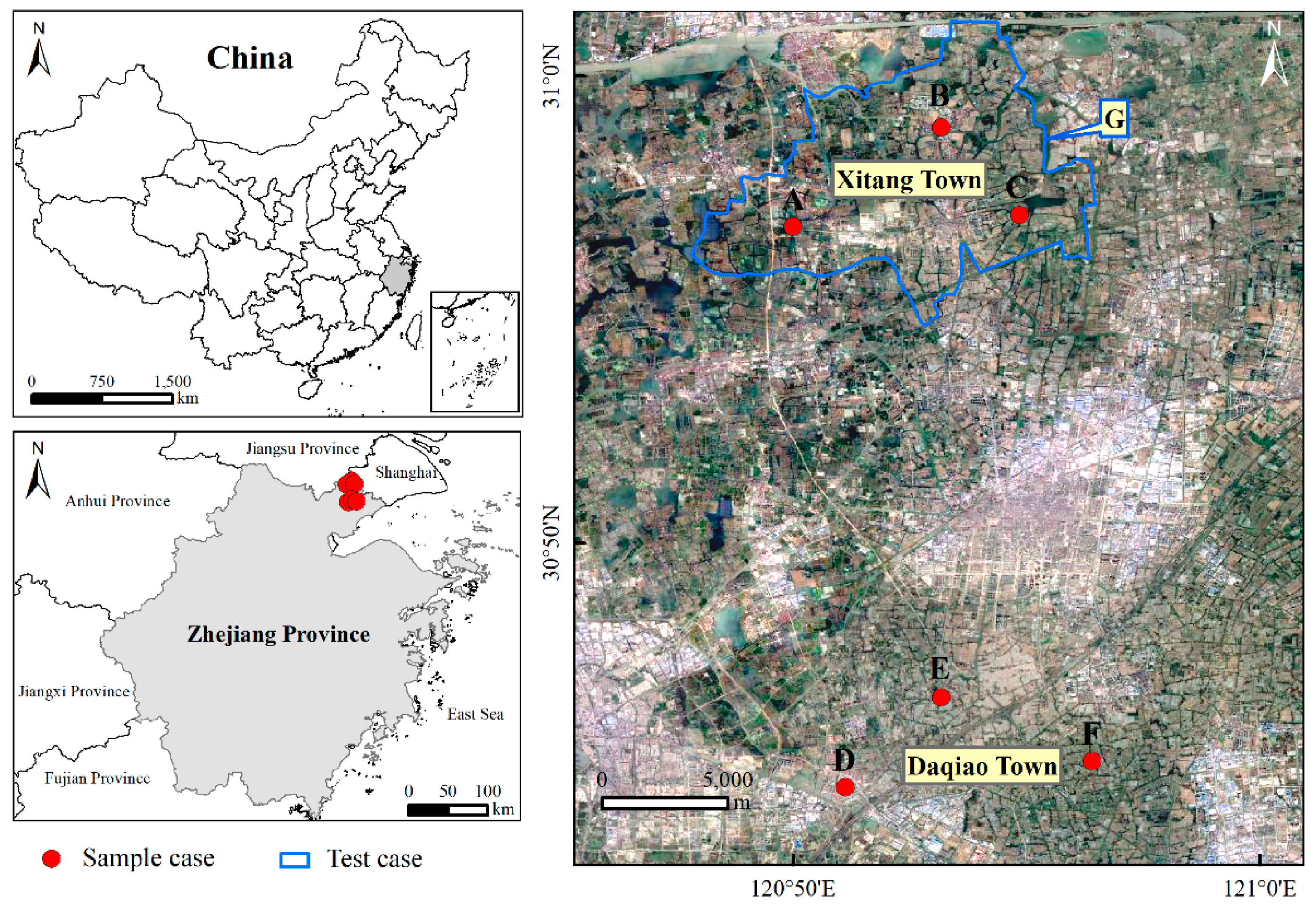
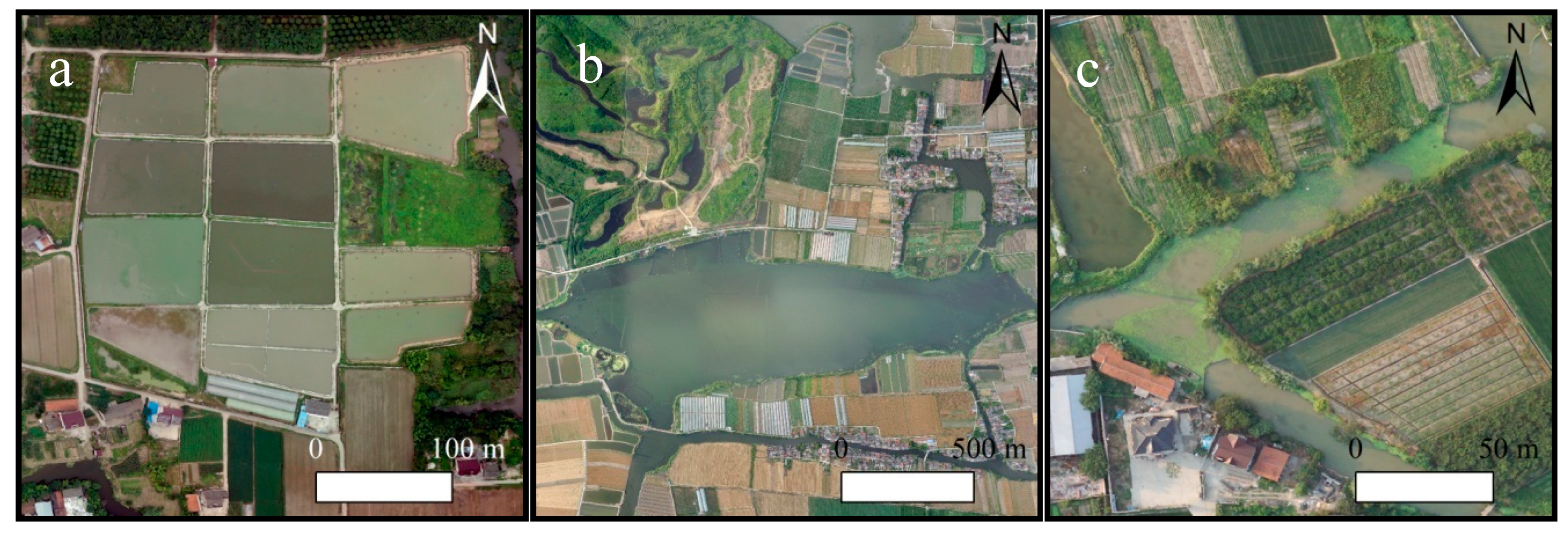
A large area of remote sensing image data was collected in Jiaxing City, Zhejiang Province, China by using a small UAV, and 6 regions were selected as experimental areas. Based on the data, the robustness and applicability of the SU-Net method in water extraction were verified. In addition, UAV images of the Xitang Region in Zhejiang Province were collected to apply SU-Net water mapping in a practical environment. The image acquisition location is shown in Figure 1. The selected sites are located in the coastal areas of South China, which cover a variety of environmental types and water body landscapes, including naturally formed lakes and rivers, paddy fields, eutrophic water bodies, polluted water bodies and shadow water bodies caused by photographic lighting, as shown in Figure 2.
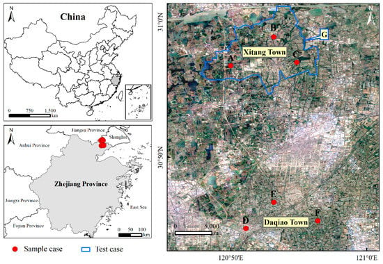
Figure 1.
Experimental sample test area and case study area. A, B, C, D, E, and F show 6 sample test areas and case areas in Xitang town (G).

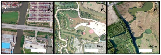
Figure 2.
Different types of water bodies obtained by wide field cameras on UAVs. (a) Paddy field, (b) lakes, (c) nutrient river, (d) sewage river, (e) park water body, and (f) shadow water body.
2.2. Data Acquisition and Preprocessing
The data collected in this paper were collected by F1000 intelligent aerial vehicles, each with a wingspan of 2.6 m and length of 1.17 m. The payload capacity of the F1000 was 4.5 kg; the cruise speed was 60 km/h; the trip duration was approximately 1.5 hours and the positioning accuracy was 5 cm. A Sony A5100 digital camera equipped with Sony E20 mm-f2.8 was selected. The design was carried out according to a resolution of 7–8 cm, with a direction overlap of 80%, a side direction overlapping degree of 60%, and an average flight altitude in the range of 350,400 m.
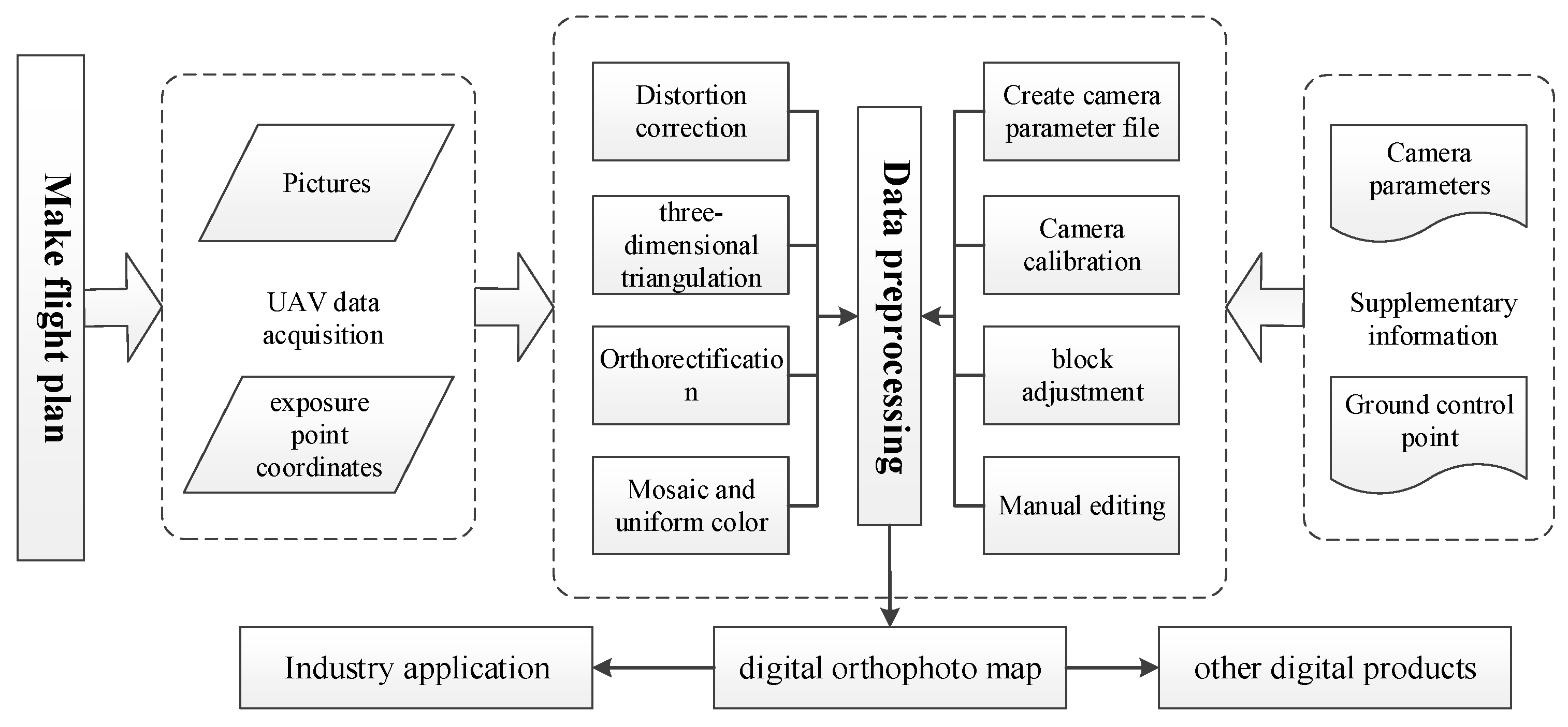
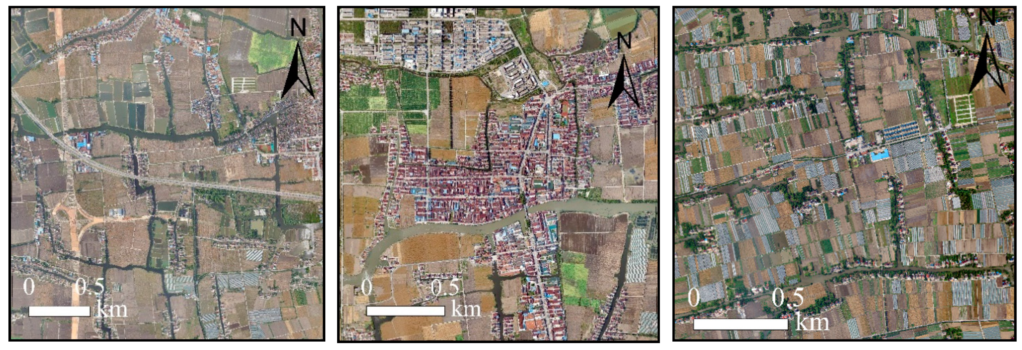
Due to the small coverage of remote sensing images acquired by UAVs, the original data comprise a series of visible images with central projections. According to the position information of the photoexposure point, it is necessary to use match, mosaic, 3D space encryption and orthorectification operations to generate ortho images [21]. Figure 3 shows the specific processing flow from the formulation of the flight plan to the generation of an orthophoto image (the relevant process is completed in ENVI5.3), which is mainly composed of three steps: formulation of the flight plan, field flight image acquisition and data correction. To obtain the image data of the whole urban area and correct the influence of weather and light on the images, it is necessary to mosaic the images of different sorties. During aerial photographing, due to changes in flight route and attitude, the optical distortion of the camera lens and other factors, the remote sensing images acquired by the UAV are irregular and have serious geometric distortions. To ensure the accuracy of position information, a whole image is adjusted by measuring the ground control points. The total area of the six test areas in this study is 28.62 km2, and the UAV images of a case study area of approximately 83.8 km2 are obtained through this data acquisition and processing method. The processing results of the three test areas are shown in Figure 4.
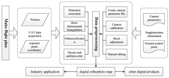
Figure 3.
Data acquisition and preprocessing.

Figure 4.
UAV orthophotos.
3. Method
3.1. Visual Feature Extraction Method for UAV Images
Due to payload limitations, UAVs usually collect three visible light bands (red, green, blue; RGB) with few spectral features. The image neighborhood features are statistically calculated in a region containing multiple pixels, which reflects the periodic change in the adjacent space of the surface. In water body recognition, this kind of regional feature has great advantages and does not cause recognition errors due to local small-scale deviations; it can therefore be applied to improve the efficiency and accuracy of water body recognition. Image textures can be calculated in many ways, such as Fourier transformations, Gabor filters [32], grey level co-occurrence matrices [33], and Gauss Markov random field mixture models [34]. These methods can be grouped into two categories: the texture calculation model based on the frequency domain and the texture calculation model based on the spatial domain. The Gabor filter has the characteristics of multichannel and multiresolution analysis, and the extracted texture features have high spatial and frequency domain resolution. The Gabor filter has good frequency, local-variation characteristics and scale changes and is representative of the frequency-domain, texture calculation model, which has been widely employed in many contexts, such as edge extraction and target recognition [35,36,37]. The GLCM is a statistical texture analysis that considers the spatial relationships among pixels; the model integrates the spatial relationships among cells into the texture analysis model with parameters such as spatial distance and angle to describe the texture characteristics of an image [38]. The GLCM is representative of the spatial texture feature quantitative model, and existing research proves that the model is an effective method for image texture analysis [39]. This paper introduces and compares two visual features based on Gabor filters and the GLCM.
3.1.1. Water Visual Feature Extraction Based on a Wavelet Transform
In all classification applications, it is necessary to analyse the spatial frequency components of images in a local, small-scale way. A two-dimensional Gabor transform was proposed in 1986 [40]. The Gabor filter function has good directional selectivity and spatial locality and can adequately describe the local grey distribution of images [41]. The advantages of the Gabor wavelet transform are mainly reflected in two aspects: (1) It has good edge sensitivity for images, can capture the spatial frequency and structural features of local images in multiple directions, and has a strong spatial discrimination ability. (2) It is insensitive to illumination changes in an image, allows the image to have a certain degree of rotation and deformation and has a certain robustness to illumination and posture. The Gabor filter is widely utilized in image processing and analysis, such as texture analysis, segmentation, and classification. Therefore, it is feasible to use a Gabor filter to calculate the texture information of water images.
In this method, a group of filters are designed to convolve an image. For different objects, due to the different frequencies and bandwidths of their grey values, the convolution results are suppressed and enhanced to different degrees. The water features are analysed and extracted from the output results of each filter for subsequent classification tasks. The Gabor transform of an image is regarded as the convolution of the image and filter function. The formula is expressed as follows:
where I(x,y) represents the original image, * represents the convolution operation, and the output after convolution is expressed in complex form [42]. The filter function is expressed as follows:
where γ is the wavelength of the filter, is the direction of Gabor wavelet, ψ is the phase offset, and is the standard deviation, which is set to 0 in this study. The ellipticity of the filter function, and hence, the ellipticity of the receptive field ellipse are determined by the parameter γ, which is referred to as the spatial aspect ratio. This paper assumes that γ is 0.5.
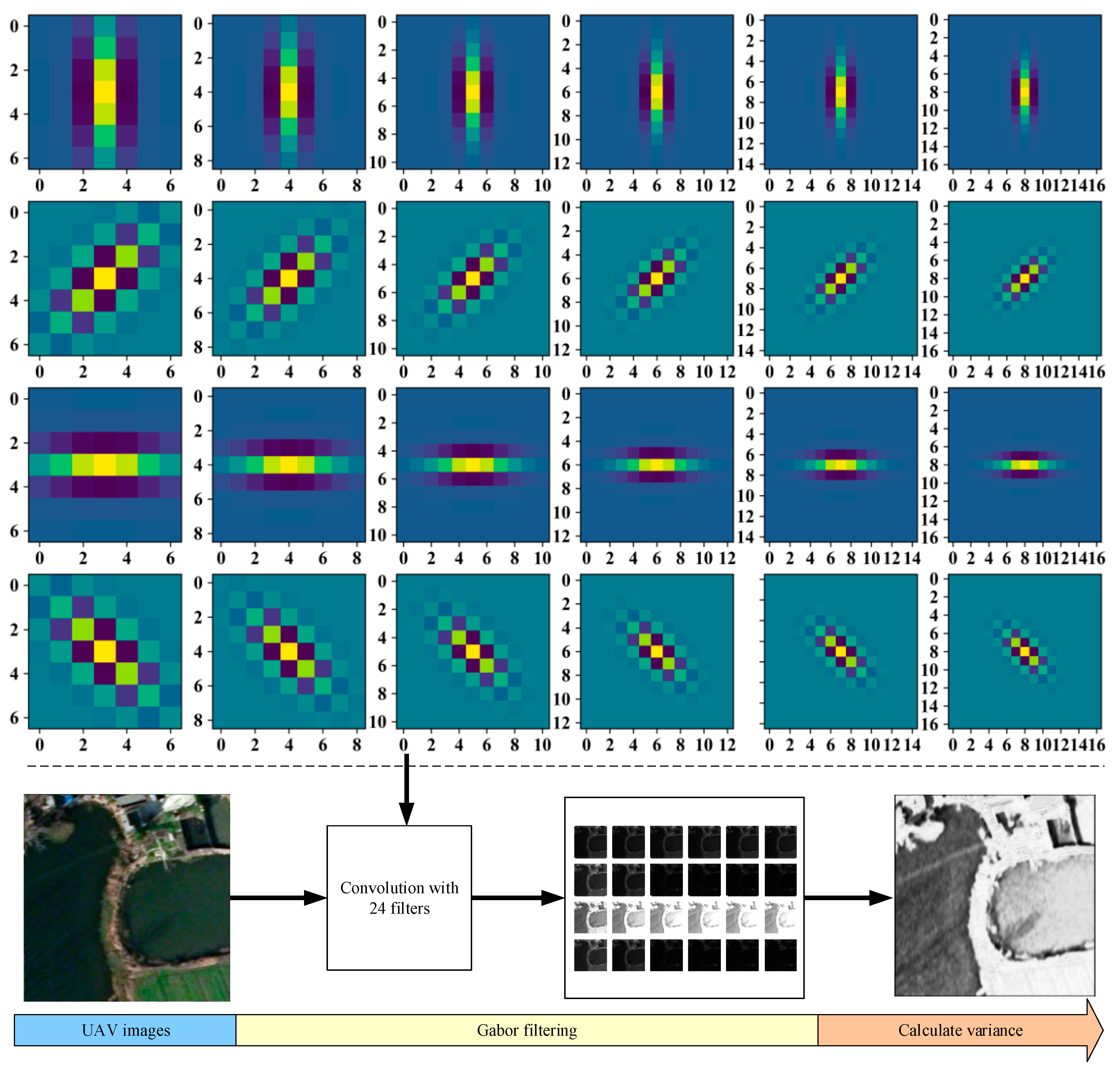
Gabor filter extraction of texture features mainly includes two processes: (1) The design filter (function, number, direction and interval). (2) The effective texture feature set is extracted from the output of the filter. Figure 5 shows the Gabor filter designed in this paper and the process of calculating the Gabor texture. The implementation steps are listed as follows:
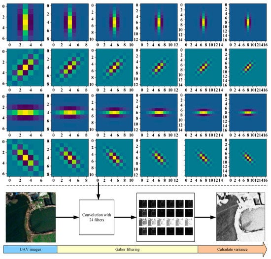
Figure 5.
Gabor filter features are calculated by convolving the images with 24 filters.
- (1)
- To establish the filter, 6 scales (6, 8, 10, 12, 14, and 16) and 4 directions (0°, 45°, 90°, and 135°) are selected. In this way, 24 filters are formed;
- (2)
- The filter is convolved with each image block in the spatial domain, and each image block can obtain 24 filter outputs.
- (3)
- Each image block passes through 24 outputs of the Gabor filter. These outputs are image block size images. If they are directly applied as feature vectors, the dimension of the feature space will be very large. In this paper, the variance in the 24 outputs is considered the texture feature value.
3.1.2. Water Visual Feature Extraction Based on the Grey Level Co-Occurrence Matrix
The statistical method of the GLCM was proposed by Haralick et al. [33] in the early 1970s. The GLCM counts the distribution of grey level values among the pixels in a grey level image. The grey level value is defined as the frequency between a pixel with a grey level value and another pixel with a corresponding grey level value. All estimated values are expressed in the form of a matrix. Because of the large dimension of the GLCM, it is generally not directly employed as a texture feature, but some statistics based on it are utilized as texture classification features. For example, Haralick proposed 14 statistics based on the GLCM: energy, entropy, contrast, uniformity, correlation, variance, sum average, sum variance, sum entropy, difference variance, difference average, difference entropy, correlation information measure and maximum correlation coefficient statistics. Entropy values show the complexity of an image. When the pixel value in the co-occurrence matrix is at the maximum randomness level, the entropy is the maximum value. In this paper, entropy is used to represent the statistics of the GLCM. The formula is expressed as follows:
where is the value of the co-occurrence matrix at (i, j).
The entropy index of the GLCM of the image centre is calculated, as shown in Figure 6. In the first step, the grey level image is compressed linearly to reduce the amount of data in the GLCM. In this paper, the grey level value is compressed in the range 0 to 8 through the linear compression method. The second step is to determine the neighborhood (n) of pixel and specify a vector with length (d) and direction (). In the third step, the GLCM is obtained by counting the number of pixel pairs on the specified vector in the neighborhood. The fourth step is to calculate the entropy value of the GLCM as a texture feature of pixel .

Figure 6.
Grey level co-occurrence matrix and entropy calculation method of pixels.
3.2. Water Detection Based on SU-Net
This section introduces the applied deep learning algorithm and the specific process of deep learning theory, including the network architecture overview, data set preprocessing, model implementation and the training process.
3.2.1. SU-Net Deep Learning Model
Assume that the input image maps to the pixel classification graph , where is the width, is the height, and is the number of input image features. For the prediction of water bodies, the output is the confidence value of the water body. The convolutional network can be described as the mapping function and is given by the following formula:
where is the parameter of the mapping function and the function can be decomposed into several subfunctions, and . By increasing the number of subfunctions, a deeper network can be obtained to enhance the fitting effect.
Therefore, the mapping function is changed into a combination of several simple subfunctions, and a multilayer deep model is obtained. The most important layer in these models is the convolution layer, which generates feature maps by convolving the input with a specified number of kernels. In addition to the convolution layer, the pooling layer is utilized to downsample the feature map. The feature graph is divided into 2 × 2 parts in space. Through this operation, the data volume of the feature graph is reduced by 75% [43].
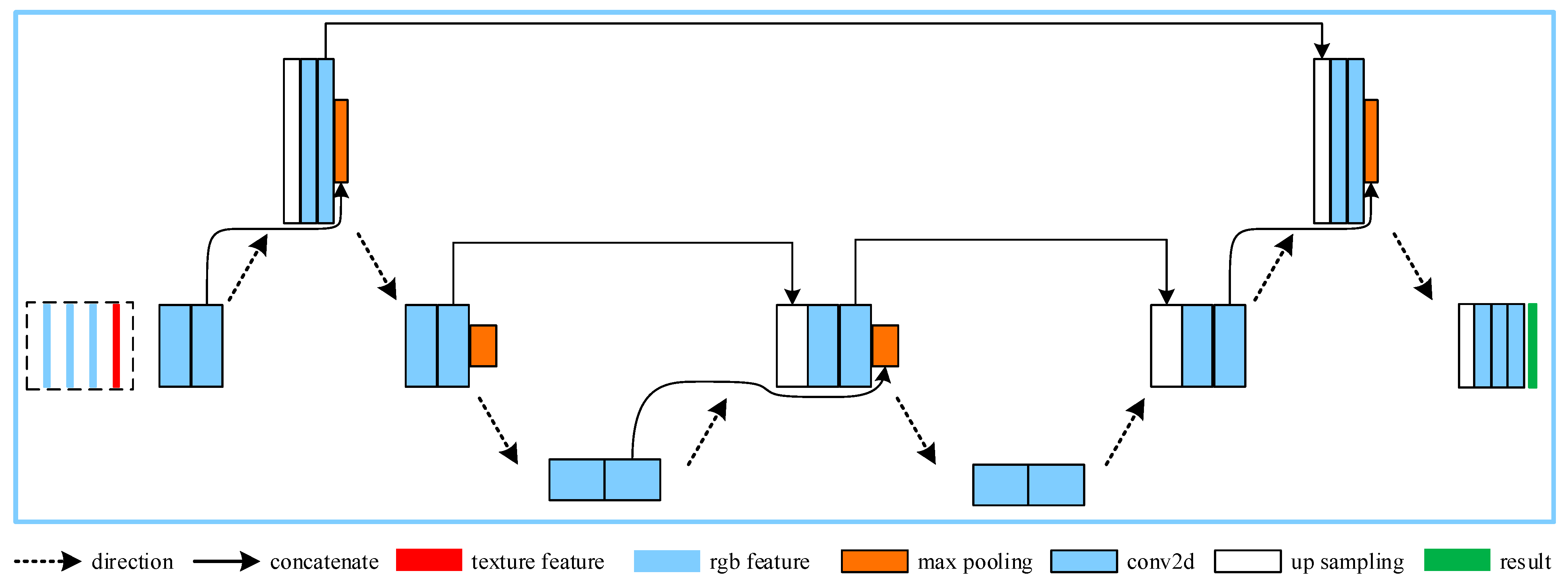
The U-Net model is widely applied in image recognition because of its low requirement on the number of training samples. In the final convolution layer, a sigmoid function is employed as the activation function to output the probability of the prediction target. The SU-Net model proposed in this paper is an improved model based on the U-Net model. Different from U-Net, pooling and upsampling are carried out alternately so that with the same number of network layers, SU-Net can achieve more fusion connections to retain more information. As shown in Figure 7, the network input layer is a image, where is the number of channels (features), and the value of is different for different experiments. Each convolution is followed by a linear function (rectified linear unit, ReLU) operation, which is merged into its corresponding convolution or deconvolution layer. The cross-operation of pooling and upsampling is performed to increase the number of layers of connections in the network. The solid arrow in Figure 7 shows all the connection operations. A larger number of connections means that more convolution features are preserved. In the final layer, a 1 × 1 convolution is used to map each eigenvector to the required number of classes. The output layer is class confidence. Therefore, each pixel has a confidence value indicating whether it is a water body.
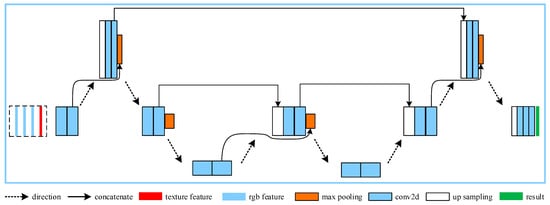
Figure 7.
SU-Net deep learning model. The arrows indicate connections, and the dotted arrows indicate the order of network operations.
3.2.2. Implementation and Model Training
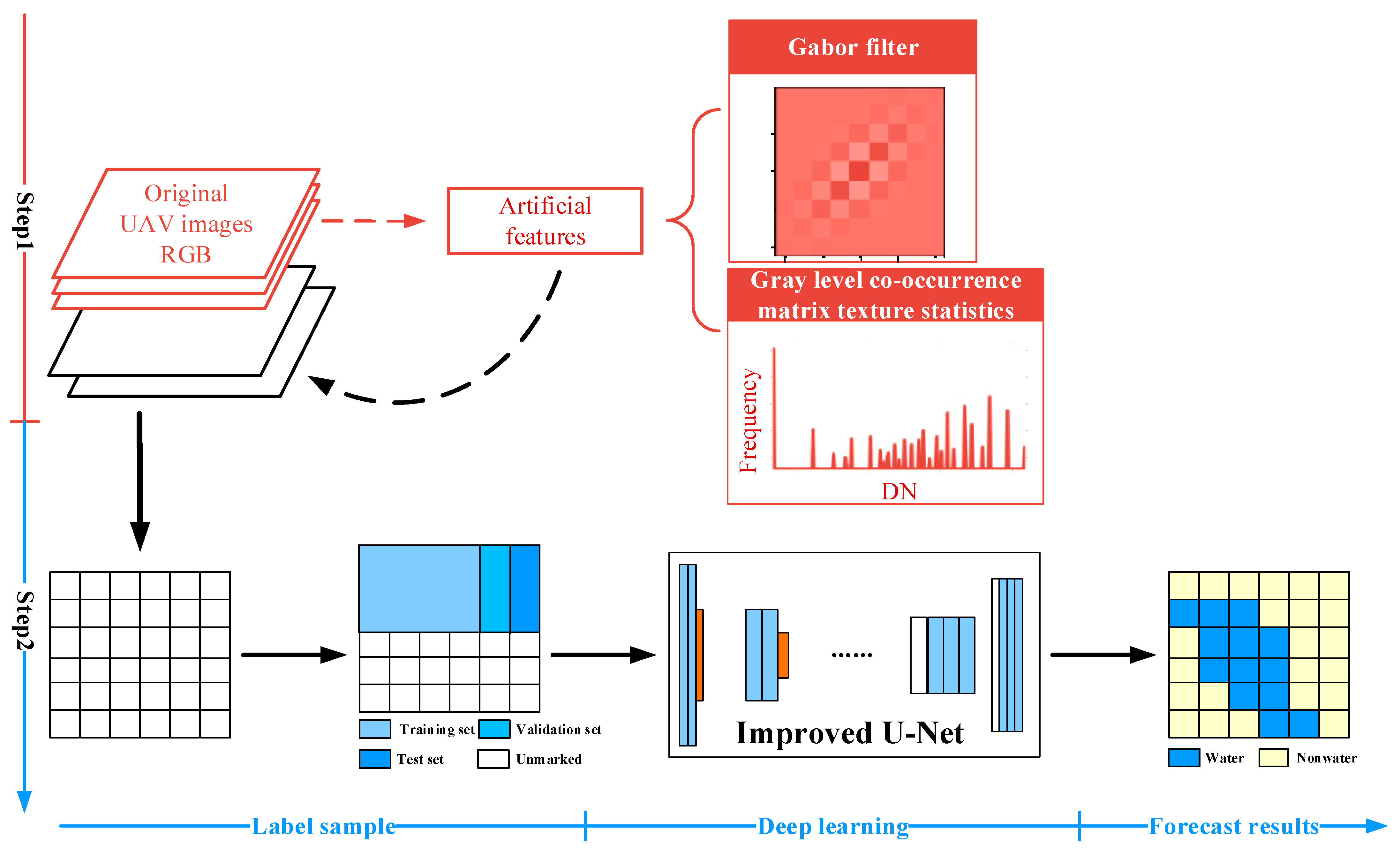
SU-Net is implemented in Keras (2.4.3), with TensorFlow (2.4.1) as the backend. This configuration is applied to all experiments in this paper. The implementation of model training is divided into three steps, as shown in Figure 8: texture feature calculation and normalization, labelling samples, training model parameters, and obtaining the prediction results.
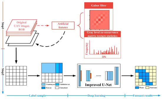
Figure 8.
Flowchart of deep learning model training.
According to the method described in 3.1, the visual characteristic value of the image in the sample area is calculated and combined with the visible light bands of the original image. Considering that the dimensions of the different features are not consistent, it is necessary to carry out histogram equalization for the combined bands and to normalize all the input data to values between 0 and 1. By comparing several normalization strategies, simple linear normalization is found to be more direct and effective.
In deep network model training, considering the limitations of hardware, the image must be divided into several small pieces and added to the training model in batches. Through a random strategy, a 256 256 area is randomly intercepted from the artificially labelled sample area as the input image of the training model and divided into a training set, verification set and test set at a ratio of 6:1:3. A total of 15,000 block samples are obtained for each test area. In this work, data enhancement mainly includes data mirroring and data flipping, which are randomly performed. The probability of mirroring, horizontal flipping and vertical flipping is 10%. This approach is particularly important when using UAV data sets for training as these enhancement methods can expand the size of training data sets. The model parameters with the minimum loss function are obtained, and the results are predicted.
In the aspect of feature combination, a larger number of features do not imply better results. The improper application of features will reduce the recognition rate of target objects. Based on the abovementioned model, the performance of several different feature combination models is analysed by inputting different feature quantities to train the models. The image features are divided into three different combinations as the input layer for experimental analysis: (I) the red (R), green (G), and blue (B) bands; (II) RGB + GLCM; and (III) RGB + Gabor.
3.3. Evaluation Metrics
In this paper, the evaluation of the model includes two aspects: the first aspect is the accuracy evaluation for measuring the closeness between the classification results of SU-Net and the real values; the second aspect is the feature applicability evaluation for determining the impact of the two texture features on the accuracy of the water extraction results.
In the process of classification, the algorithm may misclassify the background and target objects. There are four types of classification results: true positives (TP), true negatives (TN), false negatives (FN) and false positives (FP). TP is the number of positive samples that are correctly classified; TN is the number of negative samples correctly classified; FN is the number of positive samples with errors; and FP is the number of negative samples with errors [44]. These four values constitute the confusion matrix for the evaluation of the binary classification results. Based on this information, we use four measurement methods to calculate the overall accuracy (OA), precision, F-score and kappa coefficient (KC) values to evaluate the total prediction performance of the algorithm.
Accuracy is one of the most common evaluation indicators and can be used to intuitively evaluate the performance of the model. The higher the accuracy is, the better the classifier. However, in the case of unbalanced positive and negative samples, misunderstandings can occur, such as in the evaluation of a scene with almost no water. Precision represents the proportion of positive examples among the examples classified as positive examples and can represent the effect of the algorithm on water body recognition. In an actual situation, precision and recall sometimes appear contradictory. To obtain the best balance between these two indicators, the F-measure (also known as the F-score) indicator is chosen; it is the harmonic average value between precision and recall. The KC is an index for measuring the accuracy of classification. The KC is applied to determine whether the results of the model are consistent with the actual results: kappa = 1 indicates that the results are completely consistent; kappa ≥ 0.75 is considered satisfactory; and kappa < 0.4 is considered not ideal. In this paper, the OA, KC, precision and F-score are employed to compare and analyse the results of the model prediction in different situations.
4. Results
To verify the superiority of the SU-Net method, the accuracy of the water extraction results and applicability of the visual features are compared and evaluated. To evaluate the performance of the SU-Net method, we directly train the model on the RGB image of the UAV orthophoto and compare it with the standard U-Net and support vector machine (SVM) methods. Subsequently, the SU-Net model is utilized to evaluate the influence of different input feature combinations on the results of water extraction and verify the positive role of visual features in dark ground object discrimination. To prove the practical application value of this method, Xitang town, Jiaxing City, Zhejiang Province is selected as a case study to test the practical application ability of SU-Net in urban surface water mapping.
4.1. Workflow of the Experiments
The whole workflow of remote sensing image water extraction and mapping is shown in Figure 9. The process includes three steps: (1) UAV remote sensing data acquisition and visual feature calculation. (2) SU-Net deep learning model training and accuracy evaluations. (3) The application of urban water body mapping. Three steps were performed to complete the urban water mapping task. Visual feature calculation includes texture features based on a wavelet transform and statistical features based on the GLCM. Considering Xitang town in Zhejiang Province as an example, the applicability of this method is verified.
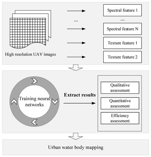
Figure 9.
Workflow of urban water body mapping.
4.2. Accuracy Evaluation
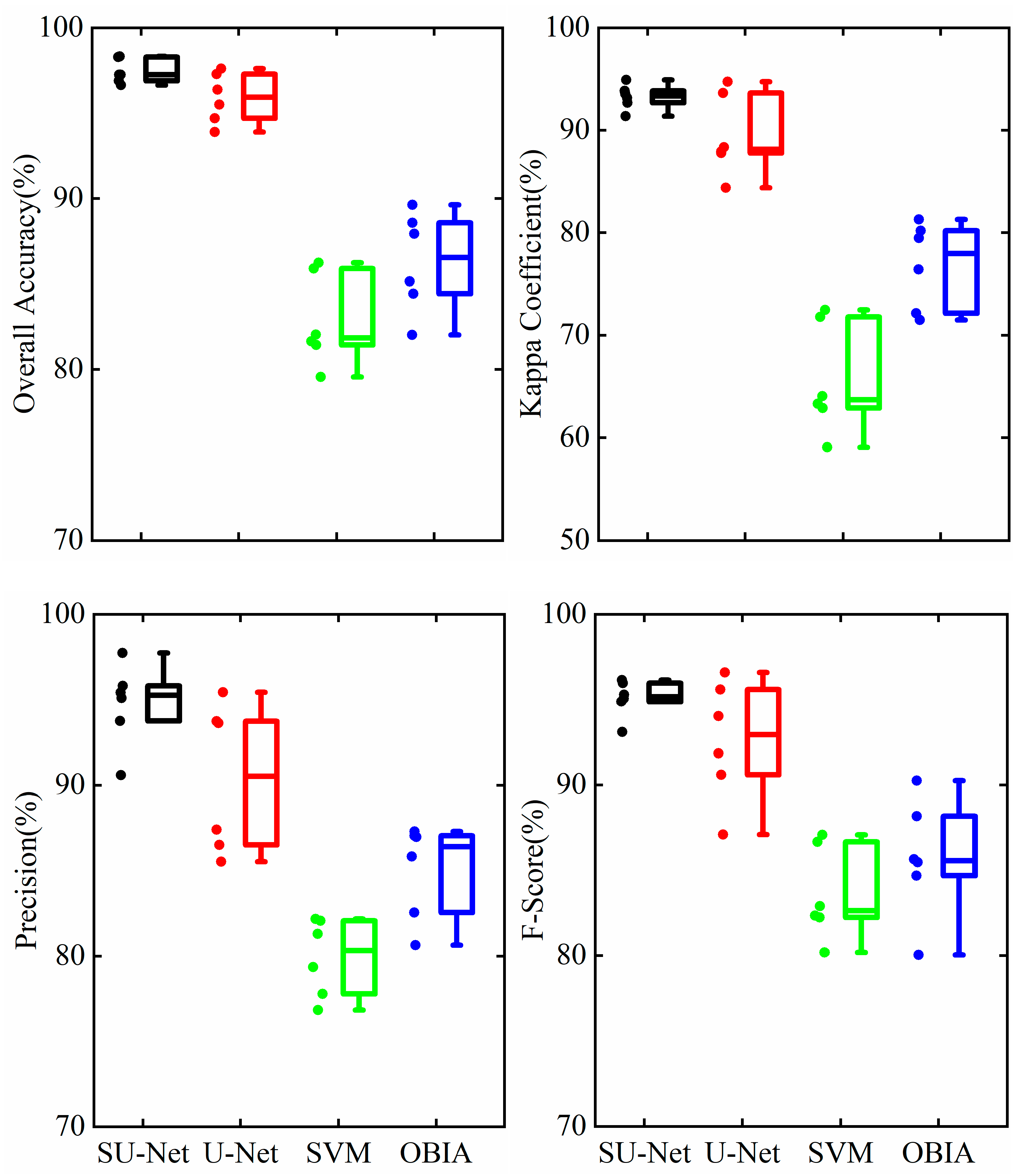
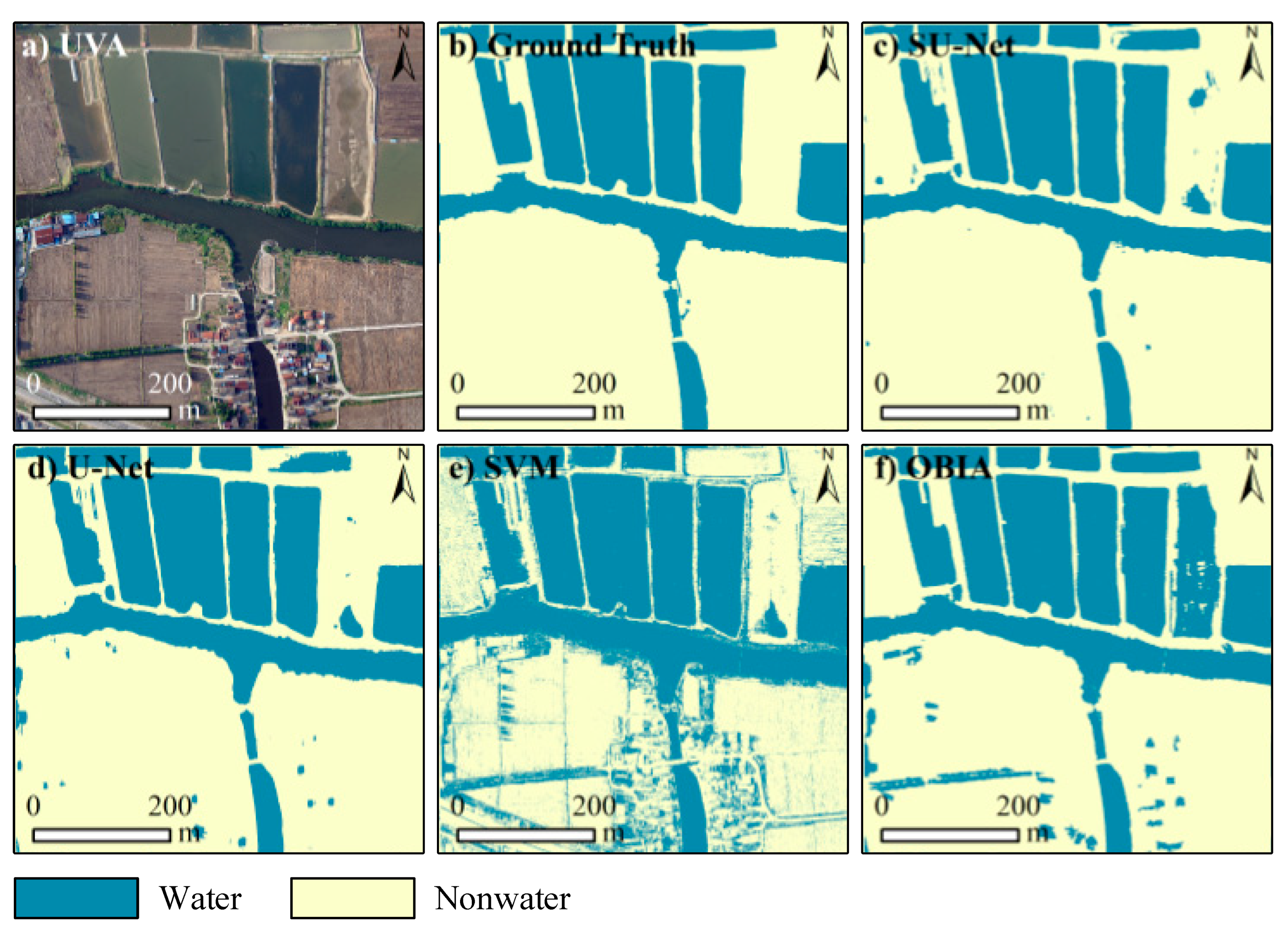
Compared with standard U-Net, SVM, and object-based image analysis (OBIA), the data set with RGB spectral features is input into the input layer and is used to quantitatively analyse the evaluation results of SU-Net. The SVM is applied in many aspects, such as building recognition, vegetation recognition, speech recognition, face recognition, and medical image recognition, and has achieved excellent results [45,46,47,48,49]. OBIA adequately achieves the recognition of patterns of homogeneous texture on images and is widely applied in classifying remote sensing images [50,51,52]. To carry out OBIA, the Example Based Feature Extraction tool in Envi 5.3 was adopted to extract water bodies in the study area. The edge segmentation method was employed to divide the image into segments, and the full lambda schedule merging method was employed to combine adjacent segments. The Scale Level and Merge Level were set to 50 and 30, respectively. For more detailed steps on OBIA, refer to our previous paper by Feng et al. [53]. Four evaluation indexes (OA, KC, F-score, and precision) of the water extraction results from different data sets were calculated in six sample test areas, as shown in Figure 10. The average values of the four evaluation indexes of the SU-Net method are higher than those of the U-Net and SVM methods. The findings conclude that the SU-Net method proposed in this paper has certain advantages.
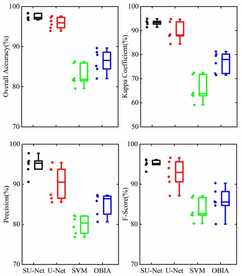
Figure 10.
Comparison of the prediction accuracy for the four methods in different data sets.
The OA value of the deep learning algorithm exceeds 90%, which is significantly higher than that of the SVM algorithm. SU-Net is the best. The median OA value of SU-Net was the highest (96.25%), with the minimum fluctuation (the standard deviation was 0.65%). The median OA value of U-Net (96.18%) was similar to that of SU-Net, but its fluctuation was large (the standard deviation was 0.94%). Although its OA (81.84%) is greater than 80%, the SVM has a low fluctuation (the standard deviation is 2.43%). The median OA of OBIA (86.54%) is better than that of the SVM, but its fluctuation (the standard deviation is 2.64%) is larger, and the total index is lower than the results of SU-Net and U-Net. Regarding OA, SU-Net has the highest accuracy and is the most stable, so it is superior to the classification methods of U-Net and the SVM.
Regarding KC, SU-Net also has the highest median KC value (93.35%) and the lowest volatility (the standard deviation is 1.08%). The maximum KC value of the U-Net method is 93.92%, but it fluctuates greatly (the standard deviation is 3.21%). The SVM and OBIA lag behind the other methods.
Regarding precision, the median values of the deep learning methods (SU-Net: 95.25% and U-Net: 92.93%) are much higher than those of the SVM and OBIA (80.33% and 86.41%). However, U-Net, the SVM, and OBIA showed large fluctuations (the standard deviations were 1.71%, 2.07%, and 2.55%, respectively).
Regarding the F-score, similar to the previous three indicators, SU-Net shows advantages in score and stability.
Combined with the classification results in Figure 11, we observe some differences in detail between SU-Net and U-Net, such as trees at the water boundary and some buildings, and the overall accuracy of SU-Net is higher than that of SVM and OBIA. SU-Net has strong advantages in the continuity of classification results. There is considerable noise in the water body recognition results of the SVM, which needs more processing in subsequent use. In the extraction of large-area water boundaries such as rivers and lakes, the water boundaries extracted by SU-Net, U-Net and OBIA are distinct, while the SVM method has irregular boundaries, which cannot be directly applied to the vector mapping of urban water boundaries.
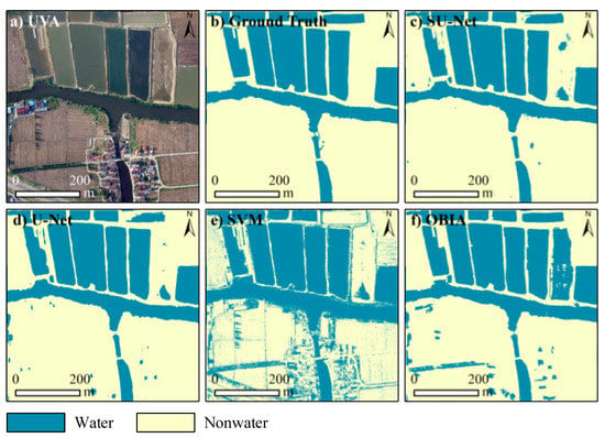
Figure 11.
Example of different methods of water body extraction results.
4.3. Applicability Evaluation of the Visual Features
Image texture and statistical information are important data sources for image classification. Based on the SU-Net method, this paper analyses the water extraction effect of two kinds of image textures, GLCM and Gabor, to evaluate the influence of the two kinds of visual feature textures and statistical features on the anti-interference and training efficiency of dark objects. Three groups of feature contrast experiments are carried out with the SU-Net model: (I) RGB, (II) RGB + GLCM, and (III) RGB + Gabor. RGB visible light is the orthophoto image acquired by the UAV, and Gabor and GLCM features are obtained by RGB calculations. The convergence rate and accuracy of the abovementioned three combined methods are tested in six experimental areas, as shown in Table 1. The results for experiment II are better than those for the other two groups in terms of the OA, KC, precision and F-score.

Table 1.
Average evaluation results of the three combined features based on SU-Net on the six data sets.
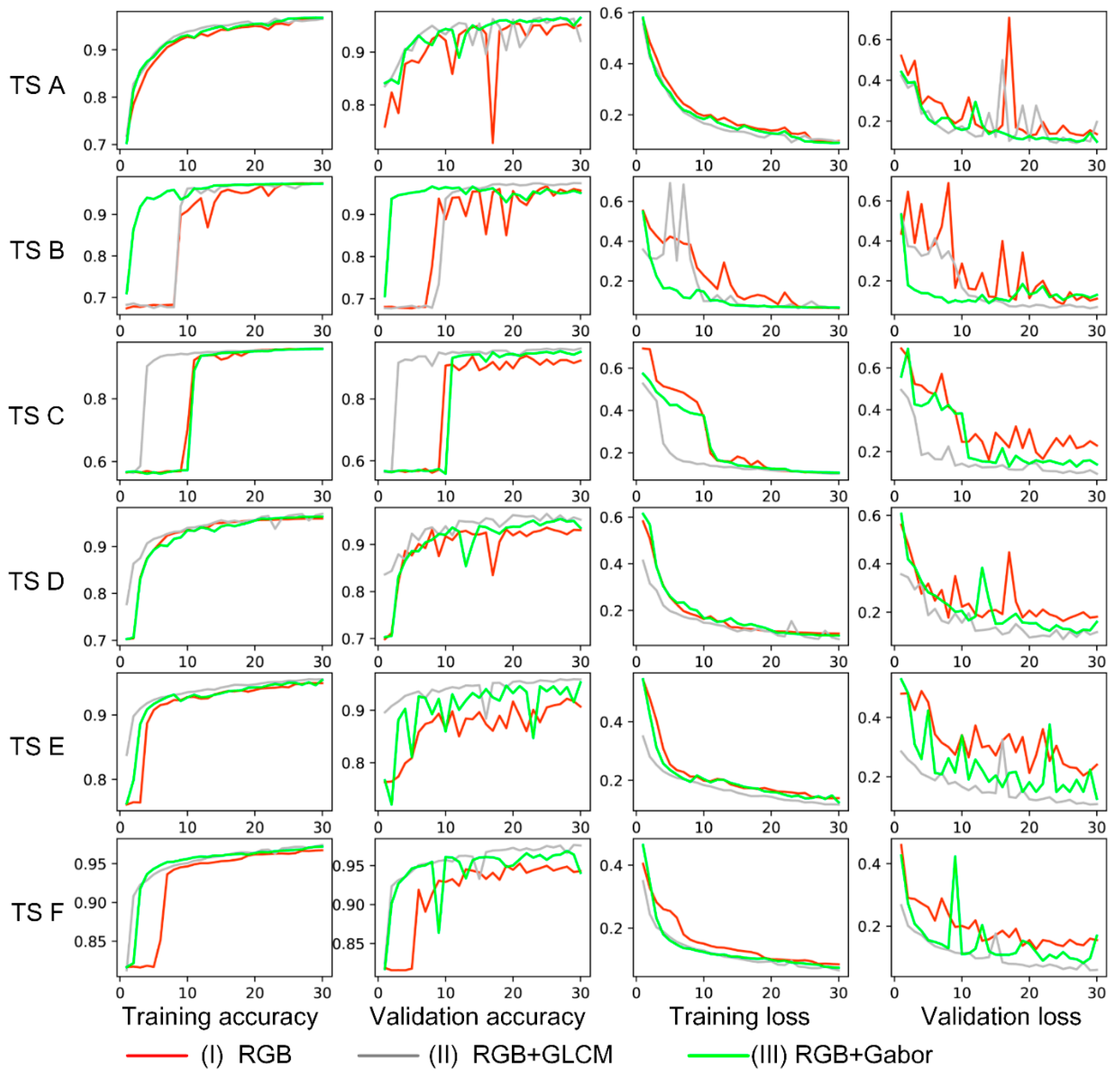
To explain the influence of the visual features on the convergence rate of the network model, 30 epochs of model training were carried out on six data sets, and the OA and loss function values of the training set and verification set in the training process were obtained. As shown in Figure 12, the accuracy values of experiments II and III with visual features in the A, D, E and F test areas converge 90% faster than those of experiment I, which indicates that visual features can positively affect the convergence speed of the deep learning model and that the accuracy is also higher than that of experiment I without visual features. Moreover, the influence of Gabor and the GLCM on the accuracy of the model is analysed. Compared with the accuracy and loss values on the validation set, the RGB + GLCM experiment shows stronger stability and smaller curve fluctuations. The other two experiments have distinct fluctuations, so the selection of appropriate visual features has a great impact on the stability of the model.
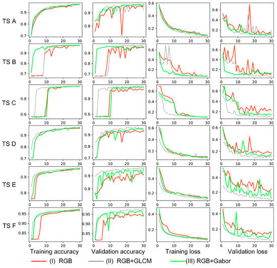
Figure 12.
Accuracy and loss values of the three experiments measured on the training set and validation set of the six experimental areas; TS represents the number of data sets.
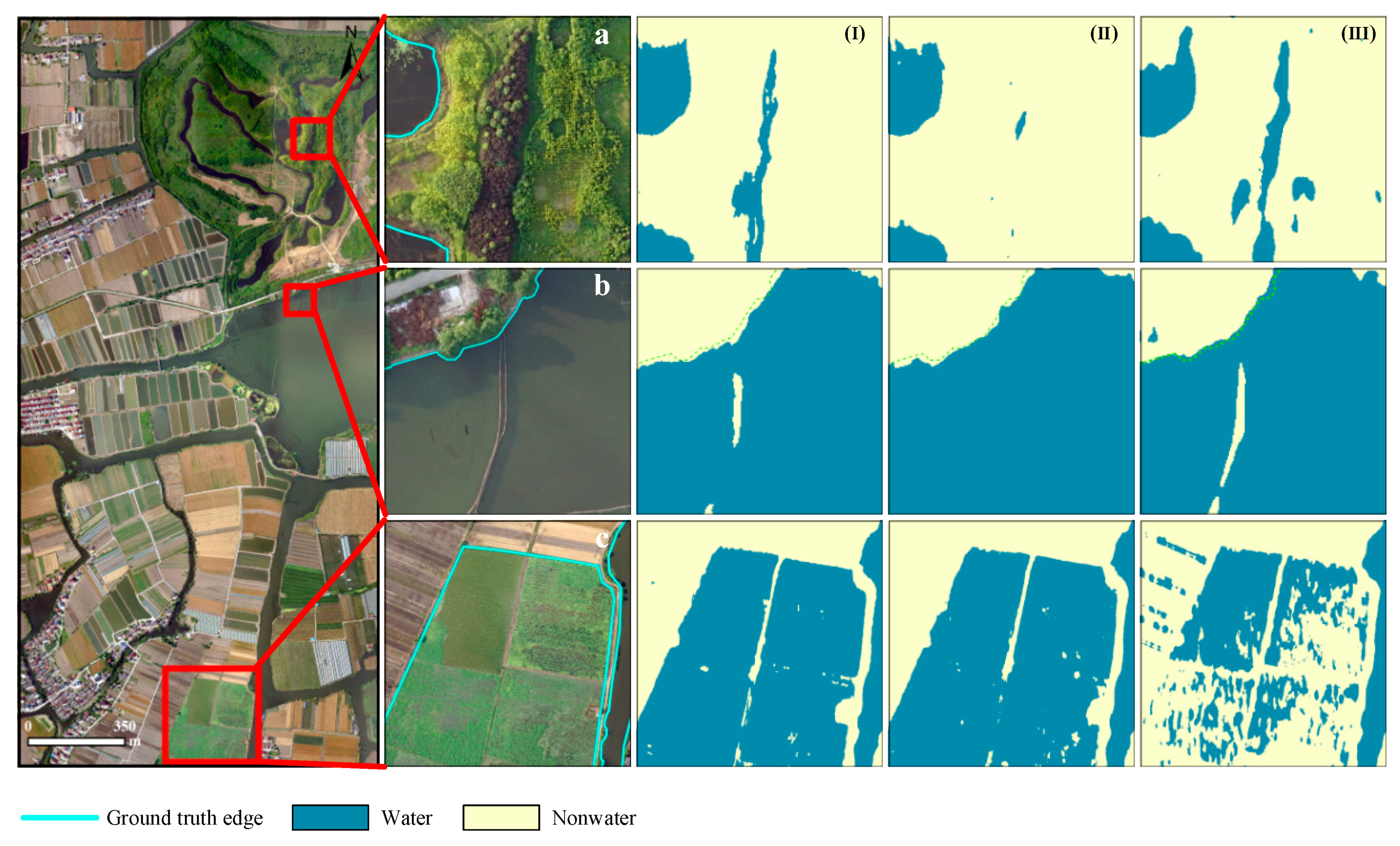
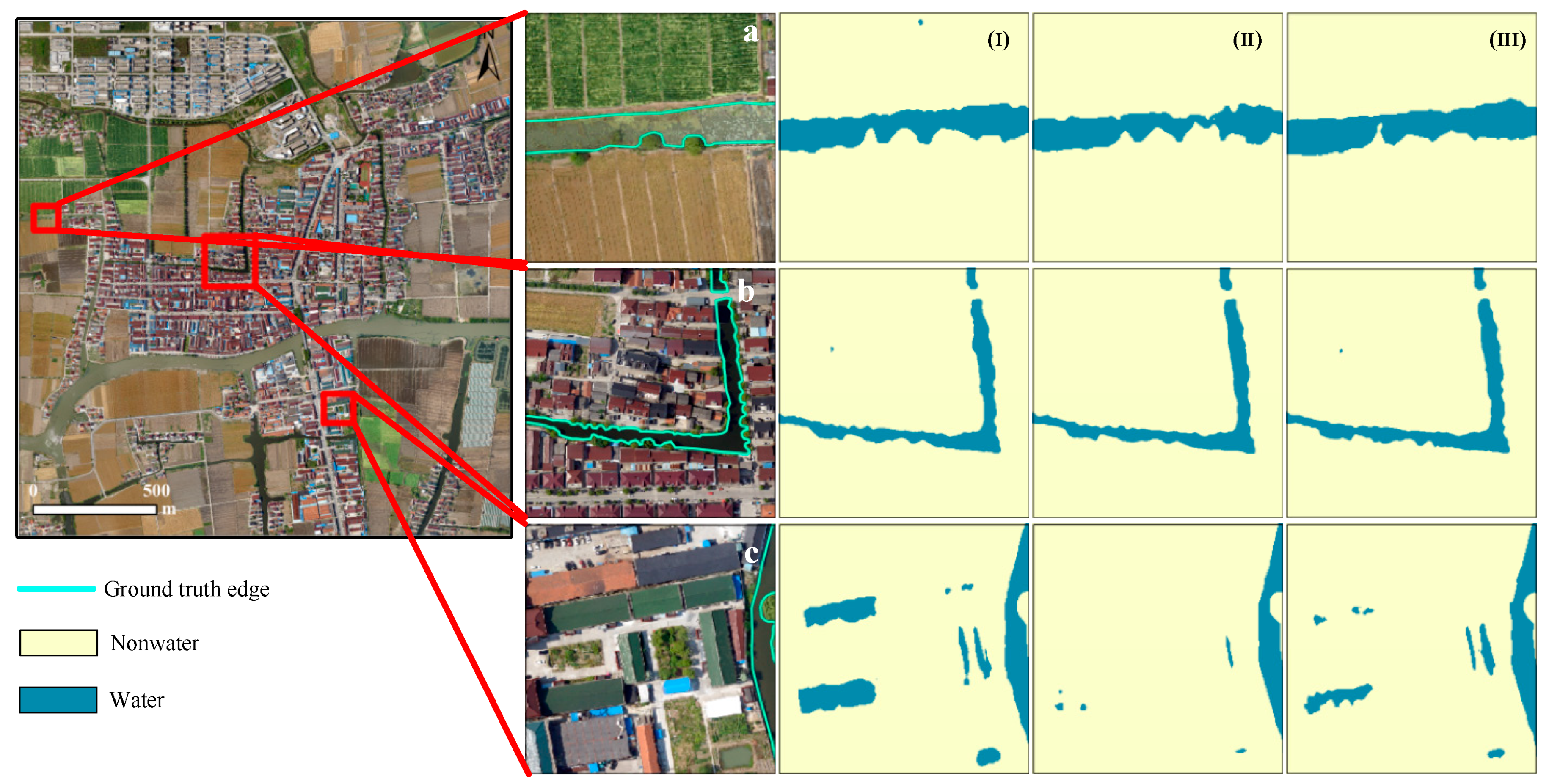
In the six test areas, we selected two representative samples to analyse the test results, as shown in Figure 13 (river and farmland area) and Figure 14 (residential area), which show the recognition results of the three experiments (RGB, RGB + GLCM, and RGB + Gabor) based on the SU-Net model for various water types. The three methods for detecting paddy fields, lakes and river water can be identified, and the paddy fields and river channels are distinct. Most of the results of water body recognition have complete boundaries and can be accurately identified for a variety of colours of water bodies. Most rivers in the region have been correctly classified, and only a few tributary ends have been disregarded or interrupted. In urban residential areas (Figure 14), the three experiments also performed well, successfully distinguishing urban roads and extracting urban water systems. However, at the level of mixed water extraction details, different visual features have different characteristics. We analyse the area from the aspects of paddy fields, shadow water, dark vegetation, nutrient water, etc. Due to the mixture of crops and water in paddy fields, the colour of paddy fields is diverse, causing paddy fields to be easily misclassified. In terms of the anti-interference ability of dark ground objects, the GLCM features of experiment II are more holistic, and the integrity of the water body is greatly improved. The extraction results are relatively complete, with more distinct boundaries and stronger robustness. Experiment II successfully distinguishes dark vegetation (Figure 13a) from dark rooftops (Figure 14c), while experiments I and III have higher misclassification rates. The dark vegetation and rooftops were mistakenly identified as vegetation. In Experiment III, the Gabor filter made the water classifier more sensitive and it could detect nonwatery pixels. Figure 13b distinguishes the isolation zone in the water, which has advantages in fine classification. However, in the extraction of paddy fields, the recognition degree of vegetation-covered water is low (Figure 13c), and the results show a certain degree of discrete state. In terms of polluted water, the method in the three experiments successfully identified the water body (Figure 14b). The RGB and RGB + Gabor experiments are affected by dark vegetation. The RGB + GLCM experiments can correctly distinguish water bodies and vegetation with low reflectance values.

Figure 13.
Comparison of water extraction results and test set details in farmland areas. From left to right, the results of water extraction in the order of experiments I, II and III are shown. (a) Dark vegetation, (b) isolation zone in the water, (c) vegetation-covered water.
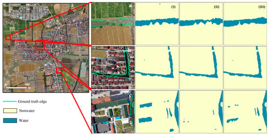
Figure 14.
Comparison of water extraction results and test set details in residential areas. From left to right, the results of water extraction in the order of experiments I, II and III. (a) Nutrient river, (b) polluted water, (c) dark rooftops.
4.4. Urban Water Body Mapping
In some cities, surface water data are updated very slowly or not at all, but this information is very important for urban development (such as flood control, land use, transportation planning, and water resource management). The water body identification method proposed in this paper can be applied to urban surface water body rendering to better understand the water body distribution in cities [54].
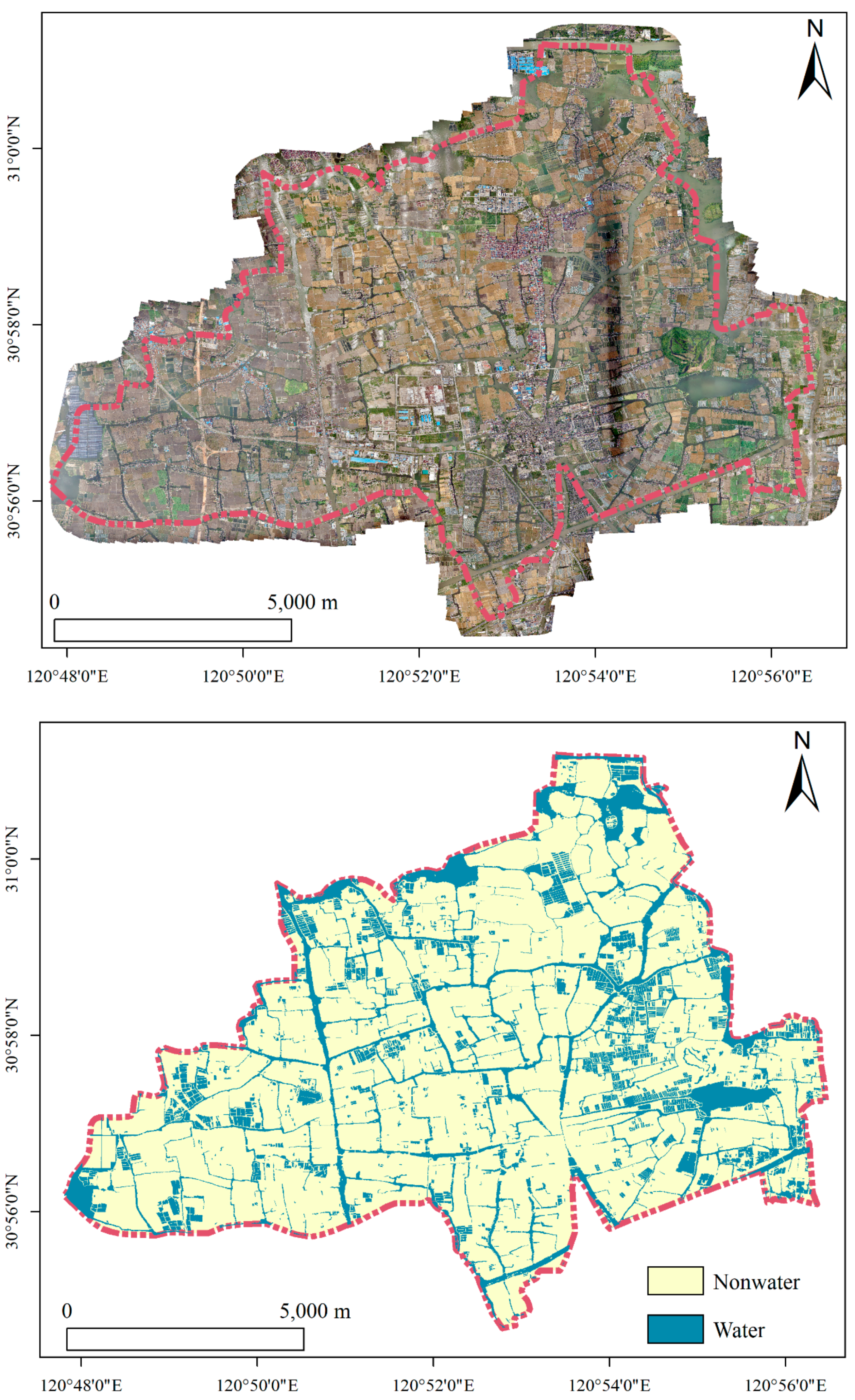
Water bodies extracted from UAV images include rivers, paddy fields, gullies, and ponds. Generally, there is a certain amount of area covered by long-term water bodies; otherwise, the water bodies easily dry up or connect with rivers. Moreover, the recognition accuracy of the deep learning model is high, so the extracted water body information has good continuity and an accurate surface area. Therefore, before urban water body mapping, the algorithm is employed to delete small, scattered areas, most of which are misclassified or temporary water bodies. Using this idea to delete scattered areas of less than 500 m2, the results of the surface water distribution map for Xitang town is shown in Figure 15. Based on the water mapping, the surface water area of Xitang town is approximately 17.37 km2, accounting for 20.72% of the total area of Xitang town. The surface water area in the east is larger than that in the west with a larger number of paddy fields.
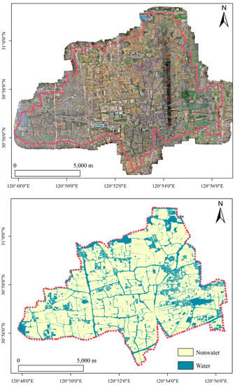
Figure 15.
Urban water body mapping.
5. Discussion
In this paper, we design a complete and effective urban water body mapping method based on UAV visible light images and propose an improved U-Net model to improve the accuracy of water body recognition. The accuracy of the model is higher than that of the conventional deep learning U-Net method. SU-Net showed the highest accuracy and robustness values for six different test data sets. Moreover, the experimental results show that UAVs are less dependent on launch and landing conditions and are not affected by a wide range of clouds, which renders them an ideal platform for urban water mapping data collection. To fully discuss the applicability of the design method, this section discusses the accuracy of water classification in mixed water and dark surface images. In addition, the shortcomings of the proposed method are pointed out, and potential improvements to the method are introduced.
5.1. Low-Precision Extraction of Mixed Surface Features and Water Bodies
A complex environment includes a mixture of land and objects, such as paddy fields with crops, edges of rivers with trees, and polluted rivers and lakes. We have observed that eutrophic water bodies or water bodies with aquatic plants (especially those covered by floating aquatic plants) are still difficult to identify by reflectivity alone. We also observed that the flashes on these water surfaces show unusually high reflectivity compared to normal water, so it is difficult to identify them. Spectral information should be applied, and other types of information sources and spatial analysis techniques should also be considered to detect them [19]. In addition, the data in this paper do not consider the continuity of rivers, which are discontinuous in areas with roads and bridges, and some rivers and other small sections may be disconnected. To solve this problem, we can revise the sample data again, replace the block with the mobile window so that each pixel has multiple classification results, and judge the final classification result according to the weight. However, this method increases the time complexity.
5.2. Interference of Shadows and Other Dark Objects on Water Extraction
Spectral features are important for using remote sensing technology to identify ground objects. For the application of water extraction in urban environments, the main factors affecting the extraction accuracy are shadows, dense vegetation, asphalt pavement and other dark objects. This finding is attributed to the notion that water and other dark objects have similar spectral characteristics in specific bands [55,56]. Therefore, water and these two objects cannot be distinguished by only their spectral characteristics. In this paper, the visual neighborhood feature enhancement algorithm based on spatial features is used to enhance the ability of the model to distinguish dark objects. Since shadows usually appear in small areas, we remove small area blocks from the results to remove the shadow pixels that are detected incorrectly. Although we successfully eliminated small shadow patches through morphological operations in our study, more data sources (such as lidar and a digital elevation model (DEM) will be added in the follow-up study and will help to improve the accuracy. This approach is our future research plan.
5.3. Expectation
Aimed at the spectral similarity problem, the combination of SU-Net and visual features can mine more information than the previous RGB space; it can effectively improve the recognition rate of low-reflective ground objects, such as mixed water and shadows, and help to accelerate the convergence speed of deep learning. Some difficulties in applying this algorithm to large-scale water information extraction still exist. In terms of the operation efficiency, expanding the research scope will inevitably increase the running time of the model, and block execution is an effective scheme. However, simplifying the time complexity of SU-Net while ensuring accuracy is an important direction of big data processing in the future. Another aspect is the cost of large-area UAV data acquisition. The combination of this method with satellite remote sensing needs further research and verification. In addition, for UAV remote sensing intermediate product data such as point clouds and DEMs, if these intermediate product data can be reasonably integrated with deep learning methods, it is believed that the spectral and spatial information of optics and point clouds can be fully mined, which will be very meaningful work.
Author Contributions
Conceptualization, W.L. and Y.L.; methodology, W.L.; software, W.L.; formal analysis, W.L.; data curation, W.H.; writing—original draft preparation, W.L.; writing—review and editing, W.L., J.G., J.Z., Q.F., J.S. and C.S. All authors have read and agreed to the published version of the manuscript.
Funding
This research was funded by the National Natural Science Foundation of China, grant number 41871323 and the Pilot Fund of Frontier Science and Disruptive Technology of the Aerospace Information Research Institute, Chinese Academy of Sciences, grant number E0Z21101.
Data Availability Statement
Data sharing was not applicable.
Acknowledgments
We thank the editor and reviewers for their valuable input and helpful comments and suggestions to significantly improve the quality of this manuscript.
Conflicts of Interest
The authors declare no conflict of interest.
References
- Ning, Z.; Li, H.; Liu, Y.; Wang, W. DEM-based extraction and analysis of digital river network of Tarim River. Water Resour. Hydropower Eng. 2020, 51, 54–61. [Google Scholar]
- Rishikeshan, C.A.; Ramesh, H. An Automated Mathematical Morphology Driven Algorithm for Water Body Extraction from Remotely Sensed Images. ISPRS J. Photogramm. Remote Sens. 2018, 146, 11–21. [Google Scholar] [CrossRef]
- Gebrehiwot, A.; Hashemi-Beni, L.; Thompson, G.; Kordjamshidi, P.; Langan, T.E. Deep Convolutional Neural Network for Flood Extent Mapping Using Unmanned Aerial Vehicles Data. Sensors 2019, 19, 1486. [Google Scholar] [CrossRef] [PubMed]
- He, Z.; Zhang, X.; Huang, Z.; Jiang, H. A water extraction technique based on high-spatial remote sensing images. J. Zhejiang Univ. Sci. Ed. 2004, 31, 701–707. [Google Scholar]
- Wang, N.; Cheng, J.; Zhang, H.; Cao, H.; Liu, J. Dynamic monitoring and application of remote sensing for aquaculture water. J. Fish. Sci. China 2019, 26, 893–903. [Google Scholar]
- Jawak, S.D.; Luis, A.J. A Rapid Extraction of Water Body Features from Antarctic Coastal Oasis Using Very High-Resolution Satellite Remote Sensing Data. Aquat. Procedia 2015, 4, 125–132. [Google Scholar] [CrossRef]
- Masocha, M.; Dube, T.; Makore, M.; Shekede, M.D.; Funani, J. Surface Water Bodies Mapping in Zimbabwe Using Landsat 8 OLI Multispectral Imagery: A Comparison of Multiple Water Indices. Phys. Chem. Earth Parts A/B/C 2018, 106, 63–67. [Google Scholar] [CrossRef]
- Yamazaki, D.; Trigg, M.A.; Ikeshima, D. Development of a Global ~90m Water Body Map Using Multi-Temporal Landsat Images. Remote Sens. Environ. 2015, 171, 337–351. [Google Scholar] [CrossRef]
- Prendes, J.; Chabert, M.; Pascal, F.; Giros, A.; Tourneret, J.-Y. Change Detection for Optical and Radar Images Using a Bayesian Nonparametric Model Coupled with a Markov Random Field. In Proceedings of the 2015 IEEE International Conference on Acoustics, Speech and Signal Processing (ICASSP), South Brisbane, Australia, 19–24 April 2015; pp. 1513–1517. [Google Scholar]
- Sumaiya, M.N.; Shantha Selva Kumari, R. Unsupervised Change Detection of Flood Affected Areas in SAR Images Using Rayleigh-based Bayesian Thresholding. IET Radar Sonar Navig. 2018, 12, 515–522. [Google Scholar] [CrossRef]
- Xie, L.; Zhang, H.; Wang, C. Water-Body Types Classification Using Radarsat-2 Fully Polarimetric SAR Data. In Proceedings of the 2015 IEEE International Conference on Aerospace Electronics and Remote Sensing Technology (ICARES), Bali, Indonesia, 3–5 December 2015; pp. 1–5. [Google Scholar]
- Kuenzer, C.; Guo, H.; Huth, J.; Leinenkugel, P.; Li, X.; Dech, S. Flood Mapping and Flood Dynamics of the Mekong Delta: ENVISAT-ASAR-WSM Based Time Series Analyses. Remote Sens. 2013, 5, 687–715. [Google Scholar] [CrossRef]
- Liao, H.-Y.; Wen, T.-H. Extracting Urban Water Bodies from High-Resolution Radar Images: Measuring the Urban Surface Morphology to Control for Radar’s Double-Bounce Effect. Int. J. Appl. Earth Obs. Geoinf. 2020, 85, 102003. [Google Scholar] [CrossRef]
- Giustarini, L.; Hostache, R.; Matgen, P.; Schumann, G.; Bates, P.; Mason, D. A Change Detection Approach to Flood Mapping in Urban Areas Using TerraSAR-X. IEEE Trans. Geosci. Remote Sens. 2013, 51, 2417–2430. [Google Scholar] [CrossRef]
- Mason, D.C.; Giustarini, L.; Garcia-Pintado, J.; Cloke, H.L. Detection of Flooded Urban Areas in High Resolution Synthetic Aperture Radar Images Using Double Scattering. Int. J. Appl. Earth Obs. Geoinf. 2014, 28, 150–159. [Google Scholar] [CrossRef]
- Shen, X.; Anagnostou, E.N.; Allen, G.H.; Robert Brakenridge, G.; Kettner, A.J. Near-Real-Time Non-Obstructed Flood Inundation Mapping Using Synthetic Aperture Radar. Remote Sens. Environ. 2019, 221, 302–315. [Google Scholar] [CrossRef]
- Sun, H.; Dai, X.; Shou, W.; Wang, J.; Ruan, X. An Efficient Decision Support System for Flood Inundation Management Using Intermittent Remote-Sensing Data. Remote Sens. 2021, 13, 2818. [Google Scholar] [CrossRef]
- Ji, L.; Gong, P.; Geng, X.; Zhao, Y. Improving the Accuracy of the Water Surface Cover Type in the 30 m FROM-GLC Product. Remote Sens. 2015, 7, 13507–13527. [Google Scholar] [CrossRef]
- Chen, Y.; Fan, R.; Yang, X.; Wang, J.; Latif, A. Extraction of Urban Water Bodies from High-Resolution Remote-Sensing Imagery Using Deep Learning. Water 2018, 10, 585. [Google Scholar] [CrossRef]
- Ireland, G.; Volpi, M.; Petropoulos, G.P. Examining the Capability of Supervised Machine Learning Classifiers in Extracting Flooded Areas from Landsat TM Imagery: A Case Study from a Mediterranean Flood. Remote Sens. 2015, 7, 3372–3399. [Google Scholar] [CrossRef]
- Feng, Q.; Liu, J.; Gong, J. Urban Flood Mapping Based on Unmanned Aerial Vehicle Remote Sensing and Random Forest Classifier—A Case of Yuyao, China. Water 2015, 7, 1437–1455. [Google Scholar] [CrossRef]
- Chen, F.; Chen, X.; Van de Voorde, T.; Roberts, D.; Jiang, H.; Xu, W. Open Water Detection in Urban Environments Using High Spatial Resolution Remote Sensing Imagery. Remote Sens. Environ. 2020, 242, 111706. [Google Scholar] [CrossRef]
- Lu, F.; Gong, Z. Construction of cloud-shadow-water mask based on Random Forests algorithm. Remote Sens. Land Resour. 2016, 28, 73–79. [Google Scholar] [CrossRef]
- McFeeters, S.K. The Use of the Normalized Difference Water Index (NDWI) in the Delineation of Open Water Features. Int. J. Remote Sens. 1996, 17, 1425–1432. [Google Scholar] [CrossRef]
- Sarp, G.; Ozcelik, M. Water Body Extraction and Change Detection Using Time Series: A Case Study of Lake Burdur, Turkey. J. Taibah Univ. Sci. 2017, 11, 381–391. [Google Scholar] [CrossRef]
- Yang, X.; Zhao, S.; Qin, X.; Zhao, N.; Liang, L. Mapping of Urban Surface Water Bodies from Sentinel-2 MSI Imagery at 10 m Resolution via NDWI-Based Image Sharpening. Remote Sens. 2017, 9, 596. [Google Scholar] [CrossRef]
- Fu, G.; Liu, C.; Zhou, R.; Sun, T.; Zhang, Q. Classification for High Resolution Remote Sensing Imagery Using a Fully Convolutional Network. Remote Sens. 2017, 9, 498. [Google Scholar] [CrossRef]
- Hu, W.; Huang, Y.; Wei, L.; Zhang, F.; Li, H. Deep Convolutional Neural Networks for Hyperspectral Image Classification. J. Sens. 2015, 2015, e258619. [Google Scholar] [CrossRef]
- Long, J.; Shelhamer, E.; Darrell, T. Fully Convolutional Networks for Semantic Segmentation. arXiv 2015, arXiv:1411.4038. [Google Scholar]
- Badrinarayanan, V.; Kendall, A.; Cipolla, R. SegNet: A Deep Convolutional Encoder-Decoder Architecture for Image Segmentation. IEEE Trans. Pattern Anal. Mach. Intell. 2017, 39, 2481–2495. [Google Scholar] [CrossRef]
- Ronneberger, O.; Fischer, P.; Brox, T. U-Net: Convolutional Networks for Biomedical Image Segmentation. In Medical Image Computing and Computer-Assisted Intervention—MICCAI 2015; Lecture Notes in Computer Science; Springer International Publishing: Cham, Germany, 2015; Volume 9351, pp. 234–241. ISBN 978-3-319-24573-7. [Google Scholar]
- Jain, A.K.; Farrokhnia, F. Unsupervised Texture Segmentation Using Gabor Filters. Pattern Recognit. 1991, 24, 1167–1186. [Google Scholar] [CrossRef]
- Haralick, R.M.; Shanmugam, K.; Dinstein, I. Textural Features for Image Classification. IEEE Trans. Syst. Man Cybern. 1973, SMC-3, 610–621. [Google Scholar] [CrossRef]
- Yu, P.; Zhang, Z.-L.; Hou, Z.-Q. Textured Image Segmentation Based on Gauss Markov Random Field Mixture Model. Acta Geod. Cartogr. Sin. 2006, 35, 224–228. [Google Scholar]
- Jain, A.K.; Ratha, N.K.; Lakshmanan, S. Object Detection Using Gabor Filters. Pattern Recognit. 1997, 30, 295–309. [Google Scholar] [CrossRef]
- Gopi, K. Fingerprint Recognition Using Gabor Filter And Frequency Domain Filtering. IOSR J. Electron. Commun. Eng. 2012, 2, 17–21. [Google Scholar] [CrossRef]
- Tamilselvi, P.R.; Thangaraj, P. Improved Gabor Filter for Extracting Texture Edge Features in Ultrasound Kidney Images. Mod. Appl. Sci. 2010, 4, 62. [Google Scholar] [CrossRef][Green Version]
- Mohanaiah, P.; Sathyanarayana, P.; Gurukumar, L. Image Texture Feature Extraction Using GLCM Approach. Int. J. Sci. Res. Publ. 2013, 3, 1–5. [Google Scholar]
- Szczypiński, P.M.; Strzelecki, M.; Materka, A.; Klepaczko, A. MaZda—A Software Package for Image Texture Analysis. Comput. Methods Prog. Biomed. 2009, 94, 66–76. [Google Scholar] [CrossRef] [PubMed]
- Turner, M.R. Texture Discrimination by Gabor Functions. Biol. Cybern. 1986, 55, 71–82. [Google Scholar] [CrossRef]
- Bianconi, F.; Fernández, A. Evaluation of the Effects of Gabor Filter Parameters on Texture Classification. Pattern Recognit. 2007, 40, 3325–3335. [Google Scholar] [CrossRef]
- Lee, T.S. Image Representation Using 2D Gabor Wavelets. IEEE Trans. Pattern Anal. Mach. Intell. 1996, 18, 959–971. [Google Scholar] [CrossRef]
- Jeppesen, J.H.; Jacobsen, R.H.; Inceoglu, F.; Toftegaard, T.S. A Cloud Detection Algorithm for Satellite Imagery Based on Deep Learning. Remote Sens. Environ. 2019, 229, 247–259. [Google Scholar] [CrossRef]
- Wei, S.; Zeng, X.; Qu, Q.; Wang, M.; Su, H.; Shi, J. HRSID: A High-Resolution SAR Images Dataset for Ship Detection and Instance Segmentation. IEEE Access 2020, 8, 120234–120254. [Google Scholar] [CrossRef]
- Li, J.; Huang, W.; Shao, L.; Allinson, N. Building Recognition in Urban Environments: A Survey of State-of-the-Art and Future Challenges. Inf. Sci. 2014, 277, 406–420. [Google Scholar] [CrossRef]
- Akbarzadeh, S.; Paap, A.; Ahderom, S.; Apopei, B.; Alameh, K. Plant Discrimination by Support Vector Machine Classifier Based on Spectral Reflectance. Comput. Electron. Agric. 2018, 148, 250–258. [Google Scholar] [CrossRef]
- Smith, N.; Gales, M.J.F. Speech Recognition Using SVMs. In International Conference on Neural Information Processing Systems: Natural and Synthetic; MIT: Vancouver, BC, Canada, 2001; pp. 1197–1204. [Google Scholar]
- Kim, S.-K.; Park, Y.J.; Toh, K.-A.; Lee, S. SVM-Based Feature Extraction for Face Recognition. Pattern Recognit. 2010, 43, 2871–2881. [Google Scholar] [CrossRef]
- Yan, T.; Liu, Q.; Wei, Q.; Chen, F.; Deng, T. Classification of Lymphoma Cell Image Based on Improved SVM. In Advances in Applied Biotechnology; Lecture Notes in Electrical Engineering; Springer: Berlin/Heidelberg, Germany, 2015; Volume 332, pp. 199–208. [Google Scholar] [CrossRef]
- Zhang, X.; Feng, X.; Jiang, H. Object-Oriented Method for Urban Vegetation Mapping Using IKONOS Imagery. Int. J. Remote Sens. 2010, 31, 177–196. [Google Scholar] [CrossRef]
- Li, X.; Shao, G. Object-Based Urban Vegetation Mapping with High-Resolution Aerial Photography as a Single Data Source. Int. J. Remote Sens. 2013, 34, 771–789. [Google Scholar] [CrossRef]
- Laliberte, A.S.; Rango, A. Texture and Scale in Object-Based Analysis of Subdecimeter Resolution Unmanned Aerial Vehicle (UAV) Imagery. IEEE Trans. Geosci. Remote Sens. 2009, 47, 761–770. [Google Scholar] [CrossRef]
- Feng, Q.; Liu, J.; Gong, J. UAV Remote Sensing for Urban Vegetation Mapping Using Random Forest and Texture Analysis. Remote Sens. 2015, 7, 1074–1094. [Google Scholar] [CrossRef]
- Obida, C.B.; Blackburn, G.A.; Whyatt, J.D.; Semple, K.T. River Network Delineation from Sentinel-1 SAR Data. Int. J. Appl. Earth Obs. Geoinf. 2019, 83, 101910. [Google Scholar] [CrossRef]
- Chen, J.; Liu, S.; Wang, C.; You, S.; Wang, Z. Research on Urban Water Body Extraction Using Knowledge-based Decision Tree. Remote Sens. Inf. 2013, 28, 29–33. [Google Scholar]
- Xie, C.; Huang, X.; Zeng, W.; Fang, X. A Novel Water Index for Urban High-Resolution Eight-Band WorldView-2 Imagery. Int. J. Digit. Earth 2016, 9, 925–941. [Google Scholar] [CrossRef]
Publisher’s Note: MDPI stays neutral with regard to jurisdictional claims in published maps and institutional affiliations. |
© 2021 by the authors. Licensee MDPI, Basel, Switzerland. This article is an open access article distributed under the terms and conditions of the Creative Commons Attribution (CC BY) license (https://creativecommons.org/licenses/by/4.0/).

