Radiometric Normalization for Cross-Sensor Optical Gaofen Images with Change Detection and Chi-Square Test

Abstract

As the number of cross-sensor images increases continuously, the surface reflectance of these images is inconsistent at the same ground objects due to different revisit periods and swaths. The surface reflectance consistency between cross-sensor images determines the accuracy of change detection, classification, and land surface parameter inversion, which is the most widespread application. We proposed a relative radiometric normalization (RRN) method to improve the surface reflectance consistency based on the change detection and chi-square test. The main contribution was that a novel chi-square test automatically extracts the stably unchanged samples between the reference and subject images from the unchanged regions detected by the change-detection method. We used the cross-senor optical images of Gaofen-1 and Gaofen-2 to test this method and four metrics to quantitatively evaluate the RRN performance, including the Root Mean Square Error (RMSE), spectral angle cosine, structural similarity, and CIEDE2000 color difference. Four metrics demonstrate the effectiveness of our proposed RRN method, especially the reduced percentage of RMSE after normalization was more than 80%. Comparing the radiometric differences of five ground features, the surface reflectance curve of two Gaofen images showed more minor differences after normalization, and the RMSE was smaller than 50 with the reduced percentages of about 50–80%. Moreover, the unchanged feature regions are detected by the change-detection method from the bitemporal Sentinel-2 images, which can be used for RRN without detecting changes in subject images. In addition, extracting samples with the chi-square test can effectively improve the surface reflectance consistency.

1. Introduction

Presently, a huge volume of cross-sensor images is constantly acquired, which provide more valuable information for scientific research and practical application [1]. However, the different satellites have different revisit periods and swaths, so it is difficult to obtain cross-sensor images at the same date and transit simultaneously [2,3,4]. The response to the ground reflection spectrum of cross-sensor images is different at the same ground objects, which results in differences in surface reflectance obtained by cross-sensor images [5,6]. In addition, the surface reflectance consistency between cross-sensor images determines the accuracy of change detection [7], classification [8], and land surface parameter inversion [9], which is the most widespread application. Therefore, the radiometric correction is an essential preprocessing step to reduce the radiometric differences before the joint application of multi-source satellite images, such as multi-source image analysis and Earth monitoring [10,11].

Radiometric correction is divided into two types: absolute correction and relative normalization [12]. Absolute correction includes two steps of absolute radiometric calibration (ARC) and atmospheric correction. ARC aims at converting the digital number (DN) image into the meaningful physical quantities of Top-Of-Atmosphere (TOA) radiance, and atmospheric correction converts the TOA radiance into surface reflectance values [12,13]. Usually, relative normalization aims at normalizing the DN values of the subject image to match a reference image. The directly normalizing method does not fully consider the physical factors of remote sensing imaging and atmosphere condition, so it is difficult to obtain high-precision surface reflectance values [12,14]. The absolute correction combines atmosphere data and ARC parameters to fully consider various influences, such as sensor calibration, atmospheric characteristics, and illumination conditions [15,16]. Of course, any method has limited accuracy, the residual radiometric differences between cross-sensor images after absolute correction still affect the practical application [17]. To effectively and further improve the surface reflectance consistency, we combined absolute correction and relative normalization methods. First the subject and reference images are converted into surface reflectance images with ARC and atmospheric correction, and then normalize the surface reflectance values of the subject image to match a reference image.

The difficulty of the RRN method is how to automatically extract samples that can improve the surface reflectance consistency. These samples need to meet an assumption that the surface reflectance of subject images is a linear relationship to the corresponding pixels in the reference images [18,19,20]. According to the selection method for invariant and stable radiometric control set pixels, the RRN methods can be broadly classified into automatic and manual selection [21]. Since manual selection has a huge workforce cost by visual interpretation and depends on human experience and decision [18], the automatically selected method has been a hotspot [22,23]. The automatic method is divided into two categories: subtraction-based of radiometric values of two images [24] and deep learning-based method [25]. The subtraction-based methods are based on processing and analyzing the difference values of unchanged pixels pair. Such as change vector analysis (CVA) [26], principal component analysis (PCA) [27], slow feature analysis (SFA) [28], multivariate alteration detection (MAD) [29], iterative slow feature analysis (ISFA) [2], and iteratively reweighted multivariate alteration detection (IMAD) [30]. Du et al. [31] developed an objective pseudo-invariant features (PIFs) selection method with PCA and quality control. Zhong et al. [20] proposed a hierarchical regression method to extract PIFs and optimize normalization parameters for multitemporal images. Zhang et al. [32] aim to eliminate the influence of the radiometric differences in image mosaicking using the IMAD method to detect unchanged probability between reference and subject image. However, most of these methods do not consider the physical factors in subject images, directly normalize the DN values to match a reference image. This method is not conducive to obtain high-precision surface reflectance data and quantitative parameter inversion [17].

In recent years, deep learning has been a hot topic in developing new applications and has been applied in various fields, specifically remote sensing satellite images [25,33,34,35]. Today some different network models are designed for change detection, such as deep belief network (DBN) [36], generative adversarial network (GAN) [37], recurrent neural network (RNN) [38], and convolutional neural network (CNN). These networks are a supervised method that requires many training samples and only applies the coverage regions of the training sample. Therefore, we used a neural network which is an unsupervised autoencoder (AE) method, to detect changes for satellite image time series [39,40]. This method can detect permanent changes and vegetation variation that do not follow the overall tendency with the Sentinel-2 image. Compared with other unsupervised methods such as CVA, MAD, IMAD, and ISFA, this method can effectively identify entities and distinguish no-changes, seasonal changes, and non-trivial change [39,40]. We used the AE method to detect unchanged regions from the bitemporal Sentinel-2 images in RRN.

However, the unchanged regions detected by the AE method have many interference pixels that are not satisfied with the radiometric difference relationships to the corresponding pixels in the reference images. In ISFA and IMAD methods, the chi-squared test is used to iteratively reweight samples, which can effectively improve change-detection performance. Therefore, we used the chi-square test theory to construct a novel extraction (ET) method to extracting stably unchanged pixels from change-detection results instead of the iteratively reweighted (IW) for every sample. In addition, we have proved the effectiveness of extracting samples with the ET method, and it is better than the previous study of the IW method. Therefore, we use the AE and ET method implementing RRN to improve the surface reflectance consistency between cross-sensor optical Gaofen images. The main contribution is that a novel chi-square test further extracts stably unchanged samples from the unchanged regions detected by the AE method. Our method can effectively reduce the surface reflectance differences between cross-sensor optical Gaofen images.

This paper is organized as follows: Section 2 introduces the satellite image information and preprocessing steps. Section 3 explains the RRN and quantitative assessment method. Section 4 mainly proves the effectiveness of our proposed method and analyzes the RRN performance. Section 5 discusses the RNN performance in different ground features. Finally, Section 6 concludes this work.

2. Data and Preprocessing

2.1. Sentinel-2 and Gaofen Satellites

In selecting a reference image, since the ground reflective spectrum response in different sensors is different at the same ground objects, it is crucial to choose high-precision and stable data as reference images. Compared with other open access data such as Landsat and MODIS, the advantage of Sentinel-2 is the higher spatial resolution with 10 m spatial resolution in blue, green, red, and NIR bands. In addition, the surface reflectance images of Sentinel-2 can be freely downloaded or acquired using the Sen2cor toolbox to process the Level-1C data that are TOA radiance products with sub-pixel accuracy [41]. The European Space Agency provides the Sen2cor toolbox included standard algorithms to correct atmospheric effects in Sentinel-2 images, which has high accuracy and reliability [42]. Therefore, we detect unchanged regions from the bitemporal Sentinel-2 images and used one of the two images as a reference image to implement RRN in cross-sensor optical Gaofen images.

Sentinel-2 constellation has consisted of two satellites launched in 2015 and 2017 with a revisit time of 5 days, and the satellites every carry a multispectral instrument (MSI) [43].

Table 1. Bands information of Sentinel-2.

	S2A		S2B
Band	Central Wavelength (nm)	Bandwidth (nm)	Central Wavelength (nm)	Bandwidth (nm)	Spatial Resolution (m)
B1	442.7	21	442.3	21	60
B2	492.4	66	492.1	66	10
B3	559.8	36	559.0	36	10
B4	664.6	31	665.0	31	10
B5	704.1	15	703.8	16	20
B6	740.5	15	739.1	15	20
B7	782.8	20	779.7	20	20
B8	832.8	106	833.0	106	10
B8a	864.7	21	864.0	22	20
B9	945.1	20	943.2	21	60
B10	1373.5	31	1376.9	30	60
B11	1613.7	91	1610.4	94	20
B12	2202.4	175	2185.7	185	20

shows that the MSI captures 13 spectral bands from 443 nm to 2190 nm with different spatial resolutions, and it provides 10 m resolution on four bands of B2 (blue), B3 (green), B4 (red), B8 (near-infrared) [44]. Four bands usually are used for change detection, classification, and ground object recognition in optical remote sensing satellite images. The freely available Sentinel-2 products are divided into Level-1C and Level-2A. Level-1C is TOA radiance products with sub-pixel accuracy, and Level-2A is the surface reflectance data [45]. Please note that the surface reflectance values are magnified 10,000 times for numerical storage.

In this paper, we only obtained the Gaofen-1 (GF-1) and Gaofen-2 (GF-2) satellite images due to the confidentiality of national geographic information. Other optical Gaofen images, such as Gaofen-6 and Gaofen-7, are not copyright for download and purchase. However, the GF-1 and GF-2 satellites have different characteristics with imaging sensors, spatial resolution, revisit time, and orbital parameters. The cross-sensor optical images from GF-1 and GF-2 satellites can test the effectiveness of our proposed RRN method. Moreover, since the optical Gaofen images are not freely available and the copyright restrictions for purchase, we only obtain the optical Gaofen images in one region. The experiment region is located around Wuhan city center and covers various land use (e.g., deep water, shallow water, residence, road, vegetation, school, and industrial regions). There are intensive and concentrated human activities, which results in highly heterogeneous surface reflectance. Therefore, the experiment region can assess spectral characteristics with different ground features and the effectiveness of our proposed RRN method in the complex region.

The GF-1 is the first high-resolution satellite for observing Earth launched in 2013 In China, and the GF-2 is a civilian optical remote sensing satellite launched in 2014.

Table 2. Bands information of GF-1 and GF-2.

Satellite Sensor	Blue (nm)	Green (nm)	Red (nm)	Near-Infrared (nm)	Spatial Resolution (m)	Revisit Time (Day)
GF-1 PMS2	450–520	520–590	630–690	770–890	8	3–5
GF-2 PMS1	450–520	520–590	630–690	770–890	4	5

shows the wavelength range of every band, spatial resolution, and revisit time. Although the wavelength range of the two sensors is the same on every band, the surface reflectance values may be different at the same ground object due to the different atmospheric conditions, sensors, and satellite constellations [17,46]. Therefore, it is essential to normalize the surface reflectance images, which can improve the application of multi-source remote sensing images

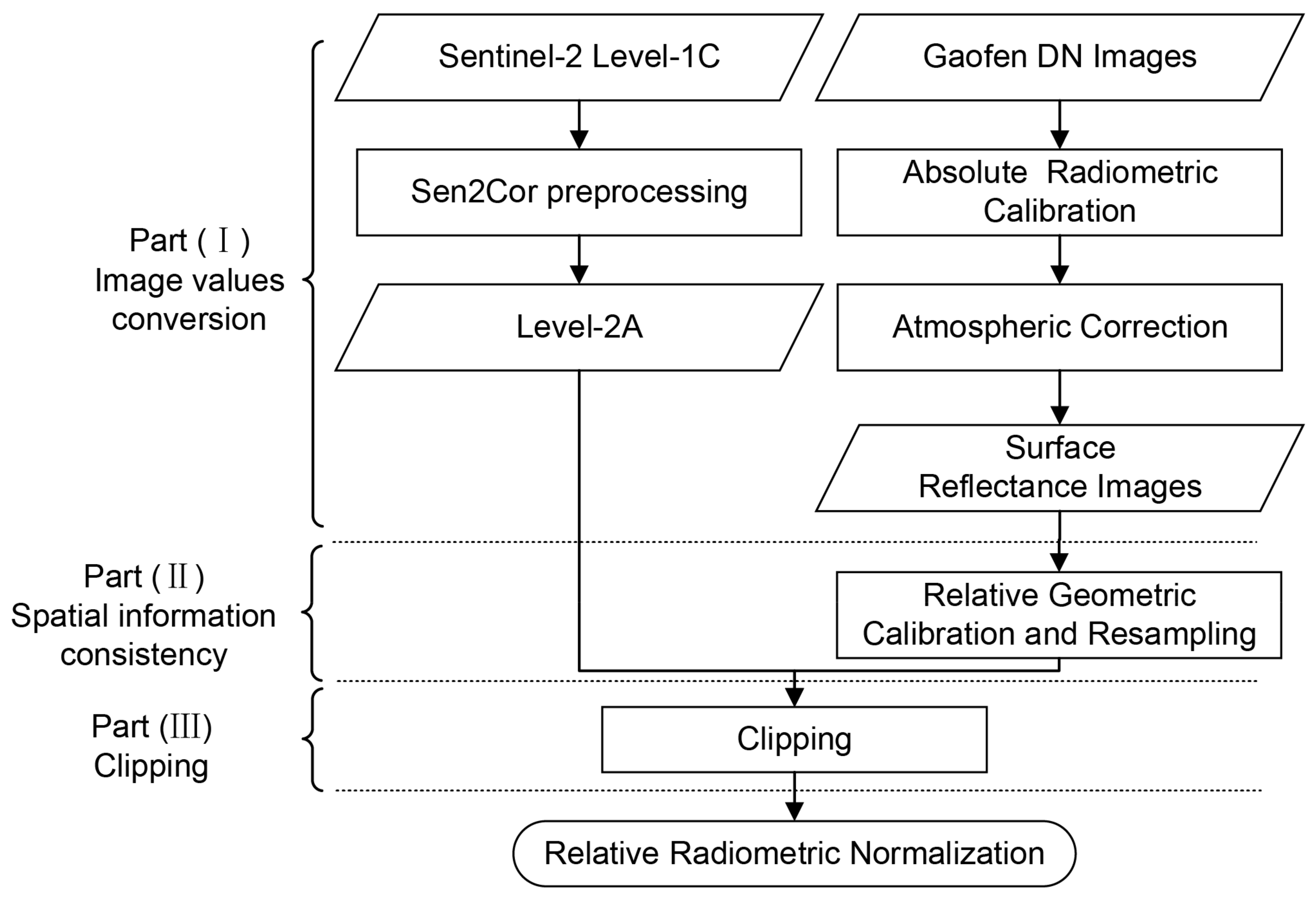
2.2. Images Preprocessing

The preprocessing step is necessary and crucial for converting the non-physical DN value into surface reflectance value to obtain the same spatial resolution and geography information between cross-sensor images. The preprocessing is divided into three parts: image values conversion, spatial information consistency, and clipping (Figure 1). For the consistency of meaningful physical quantity, the DN images should be converted into surface reflectance images by preprocessing. In reference images, we download Sentinel-2 Level-1C products [41] and use the Sen2cor preprocessing the products to obtain surface reflectance images. Since the surface reflectance products of GF-1 and GF-2 are not released, we downloaded the DN images of GF-1 and GF-2 from the China Center for Resource Satellite Data and Applications [47]. First, DN images are converted into TOA radiance using Equation (1).

$$L_j=gai{n}_j\times D{N}_j+bia{s}_j$$

(1)

where $L_j$ is the radiance which receives in the top atmospheric sensor of band $j$, $gai{n}_j$ and $bia{s}_j$ are the ARC coefficients of band $j$ (

Table 3. The ARC coefficients [48].

Satellite Sensor	Blue		Green		Red		NIR
	Gain	Bias	Gain	Bias	Gain	Bias	Gain	Bias
GF-1 PMS2	0.1490	0	0.1328	0	0.1311	0	0.1217	0
GF-2 PMS1	0.1453	0	0.1826	0	0.1727	0	0.1908	0

). Their units are $\mathrm{W}/\left({\mathrm{m}}^2·\mathrm{sr}·\mathsf{\mu }\mathrm{m}\right)$.

Then, the TOA radiance is converted into surface reflectance using the atmospheric correction algorithm that is the 6S radiative model with an open-source system [49,50,51]. Considering the geomorphic characters of the experiment area and imaging time, we chose the atmospheric model as the mid-latitude summer (MLS) model and the aerosol type as the urban type. Moreover, we set the surface reflectance model as the homogeneous Lambertian model and obtained the aerosol optical thickness (AOT) value from the AOT data in the Sentinel-2 L2A products. The spectral response matrix of GF-1 and GF-2 was resampled to 0.25 nm importing the 6S model [52]. After atmospheric correction, the surface reflectance values of the experimental images here are all magnified by 10,000 times.

For the consistency of the geography information and spatial resolution, relative geometric calibration and resampling are essential. If the spatial information errors are larger than one pixel, which would cause the mismatch of unchanged pixels between the subject with reference images, resulting in an incorrect RRN linear regression model. We manually selected 35 feature pixels in study regions to achieve the sub-pixel accuracy of relative geometric calibration base on the quadratic polynomial model and the nearest neighbor resampling method. These feature pixels include the prominent corners of ground objects such as houses, roads, and playgrounds. These ground features can effectively improve the accuracy of relative geometric calibration, and the error of that is controlled to less than 0.1 m in the north (x) and east (y) direction.

Table 4. The information of the subject and reference images after preprocessed.

Satellite Images		Geography Offset	Spatial Resolution (m)	Acquisitions Date	Image Size
Reference	S2B	2.6 m	10	12/06/2019	450 × 450
	S2A	2.6 m	10	12/11/2019	450 × 450
Subject	GF-1	3.8 m	10	12/11/2019	450 × 450
	GF-2	3.3 m	10	12/02/2019	450 × 450

shows that the geography location offset between reference and subject images meets the sub-pixel accuracy after preprocessing, less than 10 m. The offset between GF-1 and GF-2 image with S2B image is 3.8 m and 3.3 m, respectively. The geography error of S2B and S2A images is 2.6 m. Finally, clipping makes the study regions of cross-sensor optical Gaofen images consistent with the Sentinel-2 images. After preprocessing, the size and spatial resolution of cross-sensor optical Gaofen images are unified to 450 × 450 pixels and 10 m, respectively, which is consistent with the Sentinel-2 image.

3. Methodology

In this paper, we proposed an RRN method based on a change-detection method and the chi-square test to automatically extract samples, which can effectively normalize surface reflectance between cross-sensor optical Gaofen images. First, the unchanged regions are detected by the change-detection method from the bitemporal Sentinel-2 images, so we need not detect a change in subject images. Then, the chi-square test can extract the stable samples from the unchanged regions to improve the surface reflectance consistency between cross-sensor optical Gaofen images.

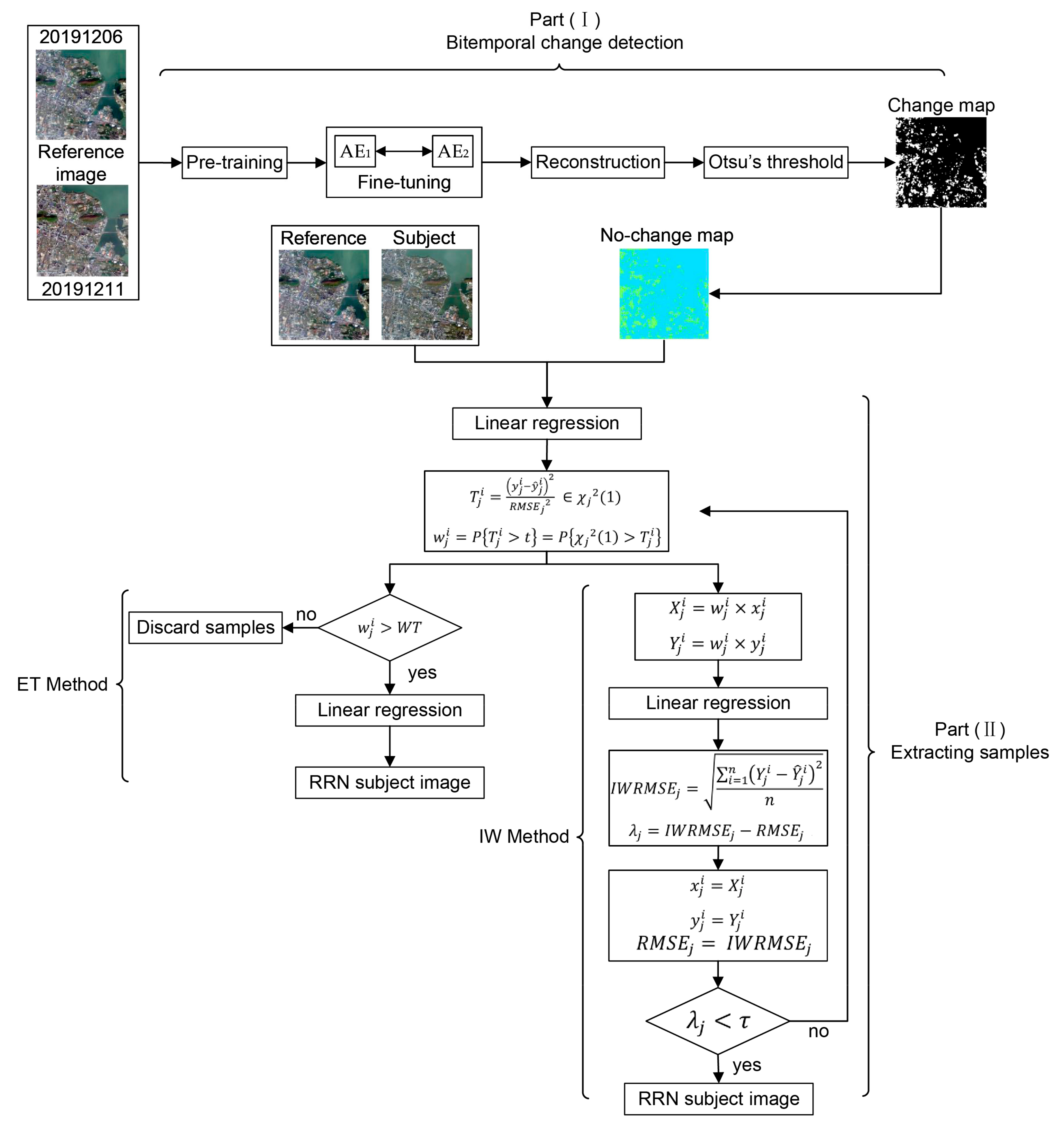
3.1. Proposed Workflow

The methodology is divided into two parts, bitemporal change detection and extracting samples with the chi-square test (Figure 2). First, we used an unsupervised autoencoder (AE) method to detect unchanged regions and generate binary change maps [39,40]. Then we used the chi-square test to construct a novel extraction (ET) method and obtain stably unchanged pixels instead of the iteratively reweighted (IW) for every sample. The IW method assigns a weight to every sample by several iterations using the chi-square test. When the difference (${\lambda }_j$) between the Iterative Weighted Root Mean Square Error ($IWRMS{E}_j$) and the previous $IWRMS{E}_j$ is less than the threshold ($\tau$) ($\tau =0.001$ in this paper), the iteration is stopped. Although the IW method does not discard any samples, the surface reflectance values have been changed by iteratively reweighted. The ET method aims at extracting stable pixels from unchanged feature regions detected by the AE method using chi-square distance as the threshold, which has not changed the surface reflectance values.

The two parts of our proposed RRN method are sketched in Figure 3. Figure 3a shows that the sky-blue square and red dot samples are the unchanged samples detected by the AE method, and the blue line (LR-1) denotes the linear regression result using these samples. Then, we used the ET method to obtain dense and stably unchanged samples shown as red dots, namely those sky-blue squares will be discarded. Finally, using these red dot samples for RRN, the black line (LR-2) denotes the final linear regression result.

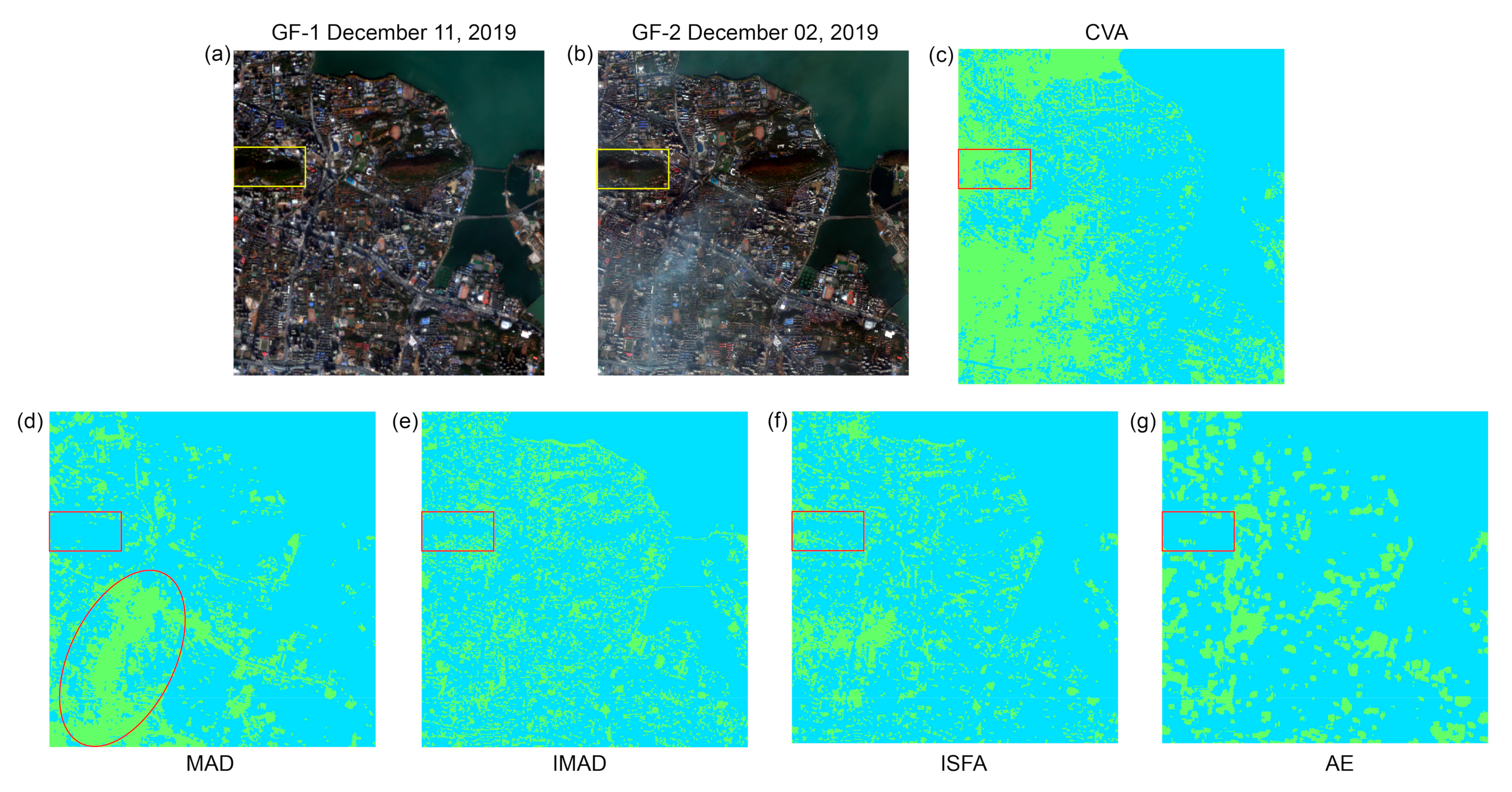
3.1.1. Bitemporal Change Detection

The AE method is the fundament of our proposed RRN method based on the reconstruction loss of the joint autoencoder model. The method can detect non-trivial changes, and it is an unsupervised method. It is mainly divided into pre-training, fine-tuning, reconstruction losses, and Otsu’s thresholding steps (Figure 2). The first step is the pre-training of the autoencoder model by encoded and decoded back every pixel pair between bitemporal images. The aim is to choose the pixel pair of the minimal difference between the decoded output and the initial input. The fine-tuning step aims to optimize every pixel pair using a joint autoencoder model composed of two autoencoders. The third step is to calculate the reconstruction error of every pixel pair. Finally, Otsu’s thresholding method detects high reconstruction errors to create a binary change map [53]. To prove whether the AE method is better than other change-detection methods, we compare the result of CVA [26], MAD [29], IMAD [30], ISFA [2] in Section 4.

3.1.2. Extracting Samples

Caselles et al. [54] verified the assumption that radiometric differences can be approximated by a linear function. However, the difficulty of RRN is how to select unchanged pixels and satisfy the assumption [18]. In the unchanged regions detected by the change-detection method, since some pixels are sparse and far from a linear function, these pixels cannot be used for linear regression in RRN. We should further extract samples from the unchanged regions to improve the RRN performance.

First, using the least square method, all pixels in the unchanged regions are used to construct a linear function and calculate the Root Mean Square Error (RMSE), which is expressed as [55]:

$${\widehat{y}}_j=a_j{x}_j+b_j$$

(2)

$${\mathrm{RMSE}}_j=\sqrt{\frac{{{\displaystyle \sum }}_{i=1}^n{\left(y_j^i-{\widehat{y}}_j^i\right)}^2}{n}}$$

(3)

where $x_j$ is the surface reflectance value of band $j$ of the subject image, ${\widehat{y}}_j$ is the surface reflectance value of the normalized image, $a_j$ and $b_j$ are linear regression coefficients. ${\widehat{y}}_j^i$ and $y_j^i$ are the surface reflectance value of sample $i$ of band $j$ of the normalized and reference image, respectively.

According to the random characteristics of the radiometric differences, we expect that every pixel pair follows a chi-square distribution with one degree of freedom [2,6]. The RMSE of linear regression is used to construct a chi-square distance as the threshold to extract samples. When the weight of samples ($w_j^i$) is larger than the weighted threshold (WT) set as 0.5 in this paper, and the sample will be preserved, otherwise discard it. The formula is expressed as:

$$T_j^i=\frac{{\left(y_j^i-{\widehat{y}}_j^i\right)}^2}{{\mathrm{RMSE}}_j{}^2} \in {\chi }_j{}^2\left(1\right)$$

(4)

$$w_j^i=P\left\{{\chi }_j{}^2\left(1\right)>T_j^i\right\}$$

(5)

$$w_j^i>WT$$

(6)

where $T_j^i$ is the chi-squared distance of sample $i$ of band $j$, ${\widehat{y}}_j^i$ and $y_j^i$ are the surface reflectance value of sample $i$ of band $j$ of the normalized and reference image, respectively. $P$ is the probability of being unchanged, measured by the probability of larger than the chi-squared distance. $w_j^i$ is the weight of sample $i$ of band $j$ same as $P$.

Finally, these extracted samples are used for linear regression with Equation (2) to normalize the surface reflectance between cross-sensor optical Gaofen images.

3.2. Quantitative Assessment

We calculate the RMSE (Equation (3)), spectral angle cosine (SAC), structural similarity (SSIM), and CIEDE2000 color-difference metrics to evaluate the performance of RRN. The RMSE and SAC can quantify the differences of surface reflectance values and spectral characteristics between two images, respectively. The smaller RMSE denotes the minor differences of surface reflectance and better the performance of RRN. In addition, if the SAC is closer to 1, the differences of spectral characteristics are smaller. The formula is defined as follows:

$$cos \alpha =\frac{{{\displaystyle \sum }}_{i=1}^n{y}_j^i{\widehat{y}}_j^i}{\sqrt{{{\displaystyle \sum }}_{i=1}^n{(y_j^i)}^2{{\displaystyle \sum }}_{i=1}^n{\left({\widehat{y}}_j^i\right)}^2}}$$

(7)

where $y_j^i$ and ${\widehat{y}}_j^i$ are the surface reflectance value of sample $i$ of band $j$ of the reference and normalized image, respectively; $\alpha$ is the spectral angle.

The SSIM and CIEDE2000 are perceptual quality assessment methods that take advantage of the know characteristics of the human visual system. The SSIM combines luminance, contrast, and structural information between two images to evaluate the similarity [56]. In addition, SSIM is very well matched to perceived visual quality compared to the peak signal-to-noise ratio (PSNR) [56,57]. The CIE published the CIEDE2000 in 2001 to quantify the color differences between two pixels [58,59]. Dionisio et al. [60] used the CIEDE2000 color difference to evaluate the spectral quality of fused remote sensing images. Therefore, we use the SSIM and CIEDE2000 color-difference (DE) metrics to evaluate the perceptual quality before and after RRN. The DE metric is based on a transformation to consider the non-uniformities of the human visual system and works in a visible color space. First, we convert three bands of Red, Green, and Blue into CIE Lab color space. In addition, then convert it to CIE LCH color space and calculate DE for every pixel pair. Finally, we calculate the average DE of all pixel pairs as a color-difference metric. If the SSIM is closer to 1, the structural similarity between the two images is higher. In addition, the smaller DE denotes the minor color differences. The SSIM and DE metrics are defined as Equation (9) [56] and Equation (10) [58,59], respectively.

$$\mathrm{SSIM}\left({\widehat{Y}}_j,Y_j\right)=f\left(l\left({\widehat{Y}}_j,Y_j\right),c\left({\widehat{Y}}_j,Y_j\right),s\left({\widehat{Y}}_j,Y_j\right)\right)$$

(8)

where ${\widehat{Y}}_j$ and $Y_j$ are the normalized and reference image of band $j$, respectively. Three functions $l\left({\widehat{Y}}_j,Y_j\right)$, $c\left({\widehat{Y}}_j,Y_j\right)$, and $s\left({\widehat{Y}}_j,Y_j\right)$ are luminance, contrast, and structural comparison functions, respectively, combined by the function $f\left(·\right)$.

$$\mathrm{DE}=\sqrt{{\left(\frac{\Delta L}{K_L{S}_L}\right)}^2+{\left(\frac{\Delta C}{K_C{S}_C}\right)}^2+{\left(\frac{\Delta H}{K_H{S}_H}\right)}^2+R_T\left(\frac{\Delta C}{K_C{S}_C}\right)\left(\frac{\Delta H}{K_H{S}_H}\right)}$$

(9)

where $\Delta L$, $\Delta C$, and $\Delta H$ are the lightness, chroma, and hue differences, respectively, calculated between the reference and normalized images. $S_L$, $S_C$, and $S_H$ are the weighting functions for the lightness, chroma, and hue components, respectively. $K_L$, $K_C$, and $K_H$ values are the parametric factors for the lightness, chroma, and hue components, respectively.$R_T$ is an interactive term between the chroma and hue differences.

4. Experiments and Analysis

4.1. Effectiveness of AE and ET Method

To evaluate the effectiveness of the AE and ET method for surface reflectance normalization, we compared five change-detection methods and the RRN performance with the chi-square test. In addition, the five different binary no-change maps were calculated by five change-detection methods, and the results of change detection were qualitatively assessed since there is no pixel-to-pixel truth change map (Figure 4). The experiment demonstrates the effectiveness of the chi-square test that can improve the radiometric consistency (Figure 5), and the ET method is better than the IW method (Figure 6).

First the binary no-change map was calculated by five change-detection methods with S2B and S2A images (Figure 4). In pre-training and fine-tuning of the AE method, the epochs were set to 1000 to determine the best train strategy. We chose ten epochs for optimal training time and loss, and the loss of pre-training and fine-tuning are 1.817 × 10⁻⁴ and 1.650 × 10⁻⁵, respectively. Figure 4c shows that the no-change map of the CVA method is too blurred to identify its ground features. Similarly, almost all unchanged samples derived by MAD concentrate in the east of Figure 4d without the clear ground feature. Generally, in good change-detection results, the unchanged samples can show the distribution of some ground features, such as lakes, lush forests, roads, and residential regions. The results of CVA and MAD show too much salt-and-pepper noise to identify the ground features, especially the CVA method. Compared to IMAD and ISFA methods, the CVA and MAD methods are short of the iterative reweighting determined by a chi-square distribution which can further screen false detections [2,30]. Therefore, IMAD and ISFA are better than CVA and MAD methods, and the lake and vegetation regions obviously show unchanged ground features (Figure 4e,f). In the red box of Figure 4f regions, the ISFA result shows that some samples are detected as changes, which may be false detections in deep-water regions. Slow feature analysis transforms the data into a new feature space to suppress the unchanged components and highlight the quickly changed components [61,62]. In deep-water regions, we speculate that some abnormal pixels belong to quickly changing in the feature space, so the differences in these pixels cannot be suppressed, resulting in false detection. Figure 4g shows that the change samples detected by AE methods are more concentrated, rather than the types of salt-and-pepper noise. The change-detection result is more consistent with the change phenomenon and identifies characteristic distributions of ground features. Some regions are unchanged ground features obviously, such as a lake, vegetation, and some impervious areas in urban areas. The CVA, MAD, IRMAD, and ISFA are subtraction-based methods to calculate the difference of every pixel pair independently. These methods cannot keep the complete shape of change ground features and are susceptible to interference from some abnormal pixels, so the change samples show the types of salt-and-pepper noise. The AE method is a neural network autoencoder algorithm, which uses patch reconstruction error instead of image difference to extract features. According to the qualitative characteristics, the AE result shows the characteristic distributions of ground features in unchanged regions, and these change samples do not show a distribution similar to salt-and-pepper noise. Therefore, we used the AE method to detect unchanged ground features for RRN.

In Figure 5, the RMSE, SAC, and SSIM curves were calculated by the normalized image and the reference image (S2B) on four bands to assess the effectiveness of the chi-square test. Since the DE works in a visible color space, we only use three bands of Red, Green, and Blue to calculate the DE curves in different change-detection methods. The different line types denote different methods, the ET and IW denote the RRN result that the chi-square test to process further unchanged samples from the change-detection results. Specifically, it denotes our proposed ET method and IW method in part (II) of Figure 2, respectively. The INC denote the RRN result using unchanged samples detected by the change-detection method without the chi-square test.

Figure 5 shows that the RMSE values of the ET and IW method are smaller than that of the INC method, and the SAC and SSIM values of the ET and IW method are larger than that of the INC method. Therefore, the chi-square test can effectively improve RRN, and the ET and IW methods are better than the INC method overall compared with the RMSE, SAC, and SSIM of five change-detection methods. Especially in the NIR band, we calculated the average values of RMSE, SAC, and SSIM of five change-detection methods. Compared with the INC method, the RMSE of GF-1 and GF-2 images was reduced by 576.538 and 605.982 (76.14 and 65.79%) using the ET method, respectively. The SAC increased by 0.018 and 0.011, and the SSIM increased by 0.093 and 0.136. The chi-square test can effectively reduce radiometric differences, and the NIR band has better performance, followed by red, blue, and green. In the GF-2 image, the RMSE of the blue band was reduced by 323.554 (73.47%), which is better than the red band (Figure 5e). Similarly, the SSIM curve shows that the performance of the blue band is better than the red band. Moreover, the DE curves significantly show that the DE values of the ET and IW method are smaller than that of the INC method, which indicates the effectiveness of the chi-square test in RRN (Figure 5d,h).

Compared to normalized and reference images, there is almost no difference between the effectiveness of the ET and IW methods. Compared with the IW method, the RMSE of the blue and red bands was reduced by 1.266 and 1.771 using the ET method, respectively. Meanwhile, the SAC increased by 3.772 × 10⁻⁵ and 5.477 × 10⁻⁴, and the SSIM curves of ET and IW methods almost overlap. Compared with the IW method, the average DE of five change-detection methods for GF-1 and GF-2 images was reduced by 0.245 and 0.282 using the ET method, respectively. However, compared with the surface reflectance differences between normalized cross-sensor optical Gaofen images, the ET method is significantly better than the IW method (Figure 6).

Figure 5 had demonstrated that the chi-square test holp to improve RRN performance. We found that the performance differences between ET and IW are very small when comparing reference with normalized images. The RMSE, SAC, and SSIM curves were calculated by two normalized images of GF-1 and GF-2 (Figure 6). The ET method is significantly better than IW compared with the radiometric differences between normalized cross-sensor optical Gaofen images, especially in the green and red bands. Other bands had also improved, i.e., the RMSE of the blue and NIR bands were reduced by10.198 and 5.041, respectively. In addition, the SAC of the blue and NIR bands increased by 5.248 × 10⁻⁴ and 6.621 × 10⁻⁴, respectively. The SSIM curve shows that the performance of ET is better than IW in the blue and green bands, but the two methods have equivalent performance in the red and NIR bands (Figure 6c). Among the five change-detection methods, the overlap of the five dashed lines demonstrates that the RRN performances are almost the same as using the IW method, but five solid lines are significantly different using the ET method and better than the IW method (Figure 6a–c). Moreover, the DE values of five change-detection methods of ET are significantly small IW, indicating the superiority of the ET method (Figure 6d). Compared with the different change-detection methods in the ET method, the AE method is slightly better than others. Therefore, in our proposed RRN method, this is also the most important reason for using the AE method to detect unchanged ground features.

As mentioned above, the main reason the change-detection performance of IMAD and ISAF methods are better than that of the CVA and MAD methods is that the CVA and MAD methods are short of the iterative reweighting determined by a chi-square distribution. Therefore, we assume that the chi-square test combining the radiometric difference function will also contribute to screening unchanged samples to improve RRN performance. The above experiments demonstrated that our assumption is feasible and effective. Moreover, the ET method is better than the IW method because the ET method further extracts stably unchanged pixels from change-detection results instead of iteratively reweighting for every unchanged pixel. The IW method has changed the surface reflectance values through iterative reweighting, which is not conducive to exclude unstably unchanged samples from change-detection results.

4.2. The Performance of Different Reference Images

In this section, we compared Sentinel-2 images with two subject images to detect unchanged regions and RRN, which assess the RRN performance of different reference images. First, the binary no-change map was calculated by five change-detection methods with two subject images of GF-1 and GF-2 (Figure 7). Then, we used the ET method to extract samples from the binary no-change map and used one of two subject images as a reference image to normalize the other image. The experiment proves that Sentinel-2 images are better than either of two subject images as reference (Figure 8). Therefore, Sentinel-2 as reference images can improve the surface reflectance consistency. The unchanged feature regions are detected by the AE method from the bitemporal Sentinel-2 images, which can be used for RRN without detecting changes in subject images.

Similarly, we found that the AE result showed the characteristic distributions of ground features in unchanged regions, and the change sample did not show a distribution similar to salt-and-pepper noise (Figure 7g). Moreover, Figure 7a,b show there are lush forests in the yellow box region where belong to unchanged ground features. Consistent with the red box of Figure 7c–g, there was detected many changed pixels by the CVA, IMAD, and ISFA methods. Figure 7d shows dense changed pixels in the red ellipse region since there has a thin cloud on the GF-2 image. Some pixels still have radiometric information in the thin cloud region, which can show the unchanged ground feature [63]. The MAD method detects some false change samples, resulting in the loss of some useful radiometric information. In summary, compared with five change-detection methods, the AE method is the most effective to detect unchanged ground features.

In Figure 8, the RMSE, SAC, SSIM, and DE curves were calculated by two normalized images of GF-1 and GF-2 to evaluate the effectiveness of using Sentinel-2 as the reference image. The different line types denote different reference images to normalize subject images. The solid line denotes the quantitative assessment that S2B and S2A images are used to detect the unchanged ground features and the S2B image as reference images to normalize GF-1 and GF-2 images. The dotted and dashed lines denote respectively GF-1 and GF-2 as reference images to normalize the other image, and the binary no-change map is calculated by GF-1 and GF-2 images. In Figure 8a–c, the different line colors and marks denote different change-detection methods.

Figure 8 shows the RMSE, SAC, SSIM, and DE curves of cross-sensor optical Gaofen images to quantitatively evaluate the RRN performance using different reference images. The RMSE both the dashed lines and dotted lines are larger than the solid lines, which implies the effectiveness of the S2B reference image is better than GF-1 and GF-2 images (Figure 8a). The SAC of the dotted lines is smaller than the dashed and solid lines, and the solid red line is the largest in the green and red bands, which are about 0.9971 and 0.9918 (Figure 8b). The SSIM of the solid lines is significantly larger than the dashed lines and dotted lines, indicating the superiority of the S2B reference image (Figure 8c). Figure 8d shows that the DE values of the S2B reference image are smaller than that of GF-1 and GF-2 reference images, which indicates that Sentinel-2 images can effectively reduce color differences between cross-sensor optical Gaofen images.

Compared with the different change-detection methods, the red dashed and dotted lines are close to the solid lines in the blue and green bands, and the RMSE of the AE method is significantly smaller than the other four change-detection methods. The solid lines show that the RMSE of five change-detection methods is almost the same, only the RMSE of the MAD method is slightly larger than others. In the blue and NIR bands, the SAC differences between five solid lines are very little, and the difference between maximum and minimum is about 0.0018. Figure 8c shows that five solid lines almost overlap, implying the same performance in five change-detection methods. However, the DE values of the five change-detection methods are different, and the IRMAD, ISFA, and AE methods are all smaller than CVA and MAD (Figure 8d). This reason may be the difference between change-detection results, and the change-detection performance of CAD and MAD is worse than the other three change-detection methods. Therefore, it is crucial to obtain good change-detection results. In summary, Sentinel-2 images and the AE method are very effective to normalize cross-sensor optical Gaofen images.

For numerical comparison of Figure 8,

Table 5. Quantitative assessment of cross-sensor optical Gaofen images normalized by different reference images.

Reference	Band	Five Change-Detection Methods Mean Value
		RMSE	SAC	SSIM
S2B	Blue	92.451	0.9976	0.3964
	Green	101.721	0.9968	0.3952
	Red	147.805	0.9913	0.4181
	NIR	353.739	0.9782	0.3358
GF-1	Blue	824.447	0.9971	0.0628
	Green	810.102	0.9930	0.0779
	Red	792.677	0.9865	0.0533
	NIR	1255.810	0.9785	0.0245
GF-2	Blue	715.083	0.9977	0.1438
	Green	798.030	0.9960	0.0845
	Red	815.662	0.9904	0.0573
	NIR	1335.977	0.9773	0.0143

shows the RMSE, SAC, and SSIM of cross-sensor optical Gaofen images normalized by different reference images. Using S2B, GF-1, and GF-2 as reference images, the RMSE is 353.739, 1255.810, and 1335.977 in the NIR band, respectively. Comparing the S2B reference image with GF-1 and GF-2 reference images, the RMSE decreased by 902.071 (71.83%) and 982.238 (73.52%), respectively. Comparing the S2B reference image with the GF-2 reference image, the SAC increased by 0.0009. Comparing the S2B reference image with the GF-1 reference image, the SAC was reduced by 0.0003. Comparing the S2B reference image with GF-1 and GF-2 reference images, the SSIM increased by 0.3313 (92.70%) and 0.3215 (95.74%), respectively. In other bands, the performance of S2B as reference images is the best. Moreover, we calculated the average DE of five change-detection methods, and the S2B reference image is smallest for 42.0451, followed by GF-2 for 48.5945 and GF-1 for 49.9487. To summarize the above experiments, the AE change-detection method and the ET method are effective for RRN, and the Sentinel-2 images can effectively reduce the surface reflectance differences between cross-sensor optical Gaofen images.

4.3. Radiometric Normalization Result

In this section, we used the AE and ET method for RRN. The above experiments had proved the effectiveness of our proposed RRN method, and the method can improve the radiometric consistency between cross-sensor optical Gaofen images. It is divided into two parts. First, the binary no-change map is calculated by the AE method using bitemporal Sentinel-2 images. Then the ET method extracts the dense and stable samples to refine the RRN linear model.

Figure 9 shows the linear regression result of the GF-1 image in every band. All different color scatters denote unchanged samples detected by the AE method, and the black line is the linear regression result using these samples. The blue, yellow and red scatters denote selected samples by the ET method, and the red line is the linear regression result using these samples. The regions with the densest numbers of samples are displayed in red, flanked by zones of yellow and blue, corresponding to declining numbers of samples. The RMSE of the red line is significantly smaller than that of the black line. In addition, the red line is closest to the red region, which indicates that the ET method can effectively discard abnormal and spare samples to improve RRN performance.

Figure 10 shows the linear regression result of the GF-2 image in every band. The RMSE of two linear regression is larger than GF-1 in every band, which may be caused by the thin clouds of the GF-2 image in the southwest [64].

The result of RRN is qualitatively analyzed by visually compared Gaofen images before and after normalization with the reference image. Five images are shown with the same linear stretch, brightness, contrast and sharpen (Figure 11). Compared to the GF-1 and GF-2 normalized image with the S2B reference image, the color and brightness of the three images are very similar. The qualitative consistency effects of the two normalized images are higher to those of the reference images than to those of the subject images. The GF-2 image still has the thin cloud in the yellow ellipse region, and this influence needs to be weakened by other methods of cloud processing [65]. In general, the radiometric consistency between the subject and reference images is greatly improved.

To numerically compare surface reflectance consistency of normalized cross-sensor optical Gaofen images,

Table 6. Quantitative assessment of cross-sensor optical Gaofen images with S2B reference images.

Satellites	Band	RMSE			SAC		SSIM
		Before	After	Rates	Before	After	Before	After
GF-1	Blue	1035.675	97.562	90.58%	0.9979	0.9977	0.5630	0.9977
	Green	1007.617	99.335	90.15%	0.9968	0.9969	0.5498	0.9970
	Red	965.953	134.187	86.11%	0.9942	0.9943	0.5128	0.9950
	NIR	1541.707	178.702	88.41%	0.9951	0.9950	0.3806	0.9924
GF-2	Blue	900.479	118.529	86.84%	0.9967	0.9967	0.6862	0.9966
	Green	1010.343	139.199	86.22%	0.9951	0.9948	0.5497	0.9952
	Red	969.920	185.729	80.85%	0.9894	0.9889	0.5127	0.9909
	NIR	1594.127	315.005	80.24%	0.9838	0.9844	0.3364	0.9766

shows the RMSE, SAC, and SSIM of the subject image before and after normalization. Three metrics were calculated by the whole image pixels between the subject and the S2B reference image. The rates are the reduced percentage of RMSE after normalization. The maximum percentage of the GF-1 and GF-2 images is 90.58% and 86.84%, respectively. In the green band, the percentage of GF-1 and GF-2 is 90.15% and 86.22%, but the SAC of the GF-2 image was reduced by 0.0003. The SSIM indicates that the blue band of the two Gaofen images is the best, 0.9977 and 0.9966, respectively. In addition, the SSIM of every band is larger than 0.9 after normalization. According to three metrics, the NIR band of the two Gaofen images is the worst. Moreover, we calculated the DE values of two Gaofen images before and after normalization. The GF-1 image before and after normalization is 47.6119 and 41.5654, and the GF-2 image is 46.8586 and 42.5957. The SSIM of the GF-1 and GF-2 was reduced by 6.0465 and 4.2629, respectively.

According to atmospheric transmission characteristics of electromagnetic waves, the atmospheric transmittance of the visible band is greater than that of the NIR band, and the transmittance of the visible wavelength of 400–700 nm is about 95%, the NIR of 700–1100 nm is about 80% [66,67]. We speculate that the difference in the atmospheric transmittance results in the different surface reflectance differences between the different bands. The greater transmittance denotes that the surface reflectance is less susceptible to atmospheric influences in satellite sensor imaging, and the surface reflectance is closer to the true ground value. Therefore, the surface reflectance differences of the NIR band are the largest both before and after normalization.

5. Discussion

Section 4 had proved the effectiveness of our proposed RRN method, and this section would discuss the RRN performance in different ground features. After normalization, the radiometric differences are different in different ground features, so the normalized accuracy is the most important for practical applications [18,68]. To evaluate the RRN effectiveness in different ground features, we have selected five regions, namely the deep water, shallow water, vegetation, building-A, and building-B (Figure 12). The deep-water region is in the Donghu lake of Wuhan, the largest lake in the city, and its depth is about 20 m. There is a scenery tourist region where the water source has always been protected. Compared with other different ground features, Figure 12b shows that three shallow water regions are colored sky-blue, two vegetation regions where are mainly evergreen broad-leaved are colored light green. In addition, two building regions are colored red and pink, respectively. The characteristic difference between the building-A and building-B regions is that the horizontal and vertical roads intersect in building-A. Both building regions are very complex and heterogeneous, covering a variety of ground features.

The surface reflectance curves were calculated by the average of all surface reflectance values in the same ground feature regions (Figure 13). The solid black line denotes the S2B reference image, and the dashed red and green lines denote the GF-1 and GF-2 images, respectively. In the legend, the RMSE was calculated by the surface reflectance curve of two images, which denotes the difference between two surface reflectance curves. Figure 13a,b shows that the curve trend of the deep water is similar to that of shallow water, but the RMSE of shallow water is smaller than that of deep water. In the reference image, the surface reflectance values of the NIR band are larger than other bands (Figure 13c). The NIR band characteristic contributes to extracting vegetation features using NDVI [69]. Similarly, the regions of building-A and building-B have this characteristic [70], while the subject images do not have this characteristic (Figure 14d,e). However, after normalization, the surface reflectance curve has a high correlation with the reference image, the GF-1 and GF-2 images also have this characteristic (Figure 14h–j).

In Figure 13f–j, RP is the reduced percentage of RMSE after normalization, and the RMSE was calculated by two surface reflectance curves of the GF-1 and GF-2 images. The RP is closer to 100%, and the reduced radiometric differences are more significant. After normalization, the surface reflectance curve of GF-1 and GF-2 is similar to the surface reflectance curve of the reference image, and the RMSE is smaller than 90. The surface reflectance curve differences are minor between GF-1 and GF-2, and the RMSE is smaller than 50 with the reduced percentages of about 50–80%. Therefore, our proposed RRN method can effectively reduce the surface reflectance differences between cross-sensor optical Gaofen images in different ground features. Especially in the deep water and vegetation regions, the normalized surface reflectance curve of the GF-1 image overlaps with that of the GF-2 images, and the RMSE is 11.740 and 14.896. Among five ground features, the maximum RP is about 82.5% in deep-water regions, and the minimum RP is about 52.9% in building-B regions. In building-B regions, the RMSE of GF-1 and GF-2 is the largest compared with other regions, which indicates that the RRN performance is less effective in the complex ground feature regions.

For numerical comparison of the RRN performance in different ground features, Figure 14 shows the quantitative assessment of RMSE, SAC, and SSIM calculated by cross-sensor optical Gaofen images and reference images. In deep water and shallow water regions, the RMSE of every band is smaller than 100 after normalization (Figure 14a,b). In the vegetation regions, the RMSE of GF-1 and GF-2 in the NIR band are 169.2 and 324.3 after normalization, equally the reduced percentage of RMSE is about 91.9% and 85.1% (Figure 14c). In two building regions, the RMSE of all bands is larger than 100 after normalization, especially the NIR band of GF-2 images, the RMSE is larger than 300 (Figure 14d,e).

Figure 14f–j shows that the SAC after normalization of every band of two images is close to 0.998 in deep water, shallow water, and vegetation regions, except the GF-2 image of the NIR band. Although the building-A regions have greatly been improved, the SAC is smaller than 0.998. The performance of the building-B regions is better than the building-A regions, but the regions need further improvement in the NIR band. Figure 14k-o shows that the SSIM significantly increases after normalization, and the GF-1 is better than GF-2.

Table 7. The DE of cross-sensor optical Gaofen images in different ground features.

Ground Features	Satellites	DE
		Before	After	Difference
Deep water	GF-1	25.5975	19.7521	5.8454
	GF-2	21.6382	12.7635	8.8747
Shallow water	GF-1	38.7180	24.7531	13.9649
	GF-2	29.5386	19.4215	10.1171
Vegetation	GF-1	54.5283	28.5795	25.9488
	GF-2	38.1057	28.2407	9.8650
Building-A	GF-1	49.7646	45.6616	4.1030
	GF-2	50.4641	45.4170	5.0471
Building-B	GF-1	48.6006	39.4771	9.1235
	GF-2	49.0103	47.9965	1.0138

shows that the DE of two Gaofen images is reduced after normalization in five ground features. The GF-1 and GF-2 of the maximum DE differences before and after normalization are about 25.9488 and 10.1171, respectively. Similarly, the RRN performance of the two building regions is worse than other homogeneous ground features.

In two building regions, the complex and multi-type land-use characteristics cause poor RRN performance, covering many heterogeneous ground features (e.g., residence, road, sparse vegetation, school, and industrial regions). In addition, the surface reflectance in these regions is greatly influenced by human activities. Since there are many mixed pixels, the radiometric difference may be nonlinear [71,72].

6. Conclusions

In this paper, we have proposed the RRN method for cross-sensor optical Gaofen images and is divided into two parts: bitemporal change detection and extracting samples. To validate the effectiveness of our proposed method, we used four metrics to quantitatively compare and analyze five change-detection methods, different reference images, and five regions with different ground features. First, the experiment demonstrates the effectiveness of the chi-square test to further extract samples for RRN, and our proposed ET method is better than the IW method. Then, the further experiment demonstrates that using Sentinel-2 as reference images can improve the surface reflectance consistency. In addition, the unchanged feature regions are detected by the AE method from the bitemporal Sentinel-2 images, which can be used for RRN without detecting changes in subject images. Four metrics demonstrated the effectiveness of our proposed RRN method, especially the reduced percentage of RMSE after normalization was more than 80%. Moreover, comparing the radiometric difference of five ground features, the surface reflectance curve of the cross-sensor optical Gaofen images showed smaller differences after normalization, and the RMSE was smaller than 50 with the reduced percentages of about 50–80%.

Our proposed RRN method can effectively reduce the surface reflectance differences between cross-sensor optical Gaofen images. We will further study improving the radiometric consistency in the heterogeneous and multi-type land-use regions and apply our RRN method into change detection using multi-source images will be the subject of our future work.

References

1. Yang, X.; Lo, C.P. Relative radiometric normalization performance for change detection from multi-date satellite images. Photogramm. Eng. Remote Sens. 2000, 66, 967–980. [Google Scholar]
2. Zhang, L.; Wu, C.; Du, B. Automatic radiometric normalization for multitemporal remote sensing imagery with iterative slow feature analysis. IEEE Trans. Geosci. Remote Sens. 2014, 52, 6141–6155. [Google Scholar] [CrossRef]
3. Collins, J.B.; Woodcock, C.E. An assessment of several linear change detection techniques for mapping forest mortality using multitemporal landsat TM data. Remote Sens. Environ. 1996, 56, 66–77. [Google Scholar] [CrossRef]
4. Song, C.; Woodcock, C.E.; Seto, K.C.; Lenney, M.P.; Macomber, S.A. Classification and change detection using Landsat TM Data: When and how to correct atmospheric effects? Remote Sens. Environ. 2001, 75, 230–244. [Google Scholar] [CrossRef]
5. Teillet, P.M. Image correction for radiometric effects in remote sensing. Int. J. Remote Sens. 1986, 7, 1637–1651. [Google Scholar] [CrossRef]
6. Moghimi, A.; Mohammadzadeh, A.; Celik, T.; Amani, M. A Novel radiometric control set sample selection strategy for relative radiometric normalization of multitemporal satellite images. IEEE Trans. Geosci. Remote Sens. 2020, 59, 2503–2519. [Google Scholar] [CrossRef]
7. Seo, D.K.; Kim, Y.H.; Eo, Y.D.; Park, W.Y.; Park, H.C. Generation of radiometric, phenological normalized image based on random forest regression for change detection. Remote Sens. 2017, 9, 1163. [Google Scholar] [CrossRef] [Green Version]
8. Friedl, M.A.; Sulla-Menashe, D.; Tan, B.; Schneider, A.; Ramankutty, N.; Sibley, A.; Huang, X. MODIS Collection 5 global land cover: Algorithm refinements and characterization of new datasets. Remote Sens. Environ. 2010, 114, 168–182. [Google Scholar] [CrossRef]
9. Nazeer, M.; Wong, M.S.; Nichol, J.E. A new approach for the estimation of phytoplankton cell counts associated with algal blooms. Sci. Total. Environ. 2017, 590–591, 125–138. [Google Scholar] [CrossRef]
10. Gens, R. Remote sensing of coastlines: Detection, extraction and monitoring. Int. J. Remote Sens. 2010, 31, 1819–1836. [Google Scholar] [CrossRef]
11. Deng, C.; Zhu, Z. Continuous subpixel monitoring of urban impervious surface using Landsat time series. Remote Sens. Environ. 2020, 238, 110929. [Google Scholar] [CrossRef]
12. Moghimi, A.; Sarmadian, A.; Mohammadzadeh, A.; Celik, T.; Amani, M.; Kusetogullari, H. Distortion robust relative radiometric normalization of multitemporal and multisensor remote sensing images using image features. IEEE Trans. Geosci. Remote Sens. 2021, 1–20. [Google Scholar] [CrossRef]
13. Janzen, D.T.; Fredeen, A.L.; Wheate, R.D. Radiometric correction techniques and accuracy assessment for Landsat TM data in remote forested regions. Can. J. Remote Sens. 2006, 32, 330–340. [Google Scholar] [CrossRef]
14. Sadeghi, V.; Ebadi, H.; Ahmadi, F.F. A new model for automatic normalization of multitemporal satellite images using Artificial Neural Network and mathematical methods. Appl. Math. Model. 2013, 37, 6437–6445. [Google Scholar] [CrossRef]
15. Hong, G.; Zhang, Y. A comparative study on radiometric normalization using high resolution satellite images. Int. J. Remote Sens. 2008, 29, 425–438. [Google Scholar] [CrossRef]
16. Rahman, M.M.; Hay, G.J.; Couloigner, I.; Hemachandran, B.; Bailin, J. An assessment of polynomial regression techniques for the relative radiometric normalization (RRN) of high-resolution multi-temporal airborne thermal infrared (TIR) imagery. Remote Sens. 2014, 6, 11810–11828. [Google Scholar] [CrossRef] [Green Version]
17. Huang, L.T.; Jiao, W.L.; Long, T.F.; Kang, C.L. A radiometric normalization method of controlling no-changed set (cncs) for diverse landcover using multi-sensor data. Int. Arch. Photogramm. Remote Sens. Spat. Inf. Sci. 2020, XLII-3/W10, 863–870. [Google Scholar] [CrossRef] [Green Version]
18. Chen, X.; Vierling, L.; Deering, D. A simple and effective radiometric correction method to improve landscape change detection across sensors and across time. Remote Sens. Environ. 2005, 98, 63–79. [Google Scholar] [CrossRef]
19. El Hajj, M.; Bégué, A.; Lafrance, B.; Hagolle, O.; Dedieu, G.; Rumeau, M. Relative radiometric normalization and atmospheric correction of a SPOT 5 time series. Sensors 2008, 8, 2774–2791. [Google Scholar] [CrossRef] [Green Version]
20. Zhong, C.; Xu, Q.; Li, B. Relative radiometric normalization for multitemporal remote sensing images by hierarchical regression. IEEE Geosci. Remote Sens. Lett. 2015, 13, 217–221. [Google Scholar] [CrossRef]
21. Schott, J.R.; Salvaggio, C.; Volchok, W.J. Radiometric scene normalization using pseudoinvariant features. Remote Sens. Environ. 1988, 26, 15–16. [Google Scholar] [CrossRef]
22. Philpot, W.; Ansty, T. Analytical description of pseudoinvariant features. IEEE Trans. Geosci. Remote Sens. 2013, 51, 2016–2021. [Google Scholar] [CrossRef]
23. Liu, S.; Marinelli, D.; Bruzzone, L.; Bovolo, F. A Review of change detection in multitemporal hyperspectral images: Current techniques, applications, and challenges. IEEE Geosci. Remote Sens. Mag. 2019, 7, 140–158. [Google Scholar] [CrossRef]
24. Bovolo, F.; Bruzzone, L. A novel theoretical framework for unsupervised change detection based on CVA in polar domain. Int. Geosci. Remote. Sens. Symp. IGARSS 2006, 45, 379–382. [Google Scholar] [CrossRef]
25. Shi, W.; Zhang, M.; Zhang, R.; Chen, S.; Zhan, Z. Change detection based on artificial intelligence: State-of-the-art and challenges. Remote Sens. 2020, 12, 1688. [Google Scholar] [CrossRef]
26. Xian, G.; Homer, C.; Fry, J. Updating the 2001 National Land Cover Database land cover classification to 2006 by using Landsat imagery change detection methods. Remote Sens. Environ. 2009, 113, 1133–1147. [Google Scholar] [CrossRef] [Green Version]
27. Deng, J.S.; Wang, K.; Deng, Y.H.; Qi, G.J. PCA-based land-use change detection and analysis using multitemporal and multisensor satellite data. Int. J. Remote Sens. 2008, 29, 4823–4838. [Google Scholar] [CrossRef]
28. Wu, C.; Du, B.; Zhang, L. Slow feature analysis for change detection in multispectral imagery. IEEE Trans. Geosci. Remote Sens. 2013, 52, 2858–2874. [Google Scholar] [CrossRef]
29. Nielsen, A.; Conradsen, K.; Simpson, J.J. Multivariate alteration detection (MAD) and MAF postprocessing in multispectral, bitemporal image data: New approaches to change detection studies. Remote Sens. Environ. 1998, 64, 1–19. [Google Scholar] [CrossRef] [Green Version]
30. Canty, M.J.; Nielsen, A.A. Automatic radiometric normalization of multitemporal satellite imagery with the iteratively re-weighted MAD transformation. Remote Sens. Environ. 2008, 112, 1025–1036. [Google Scholar] [CrossRef] [Green Version]
31. Du, Y.; Cihlar, J.; Beaubien, J.; Latifovic, R. Radiometric normalization, compositing, and quality control for satellite high resolution image mosaics over large areas. IEEE Trans. Geosci. Remote Sens. 2001, 39, 623–634. [Google Scholar] [CrossRef]
32. Zhang, Y.; Yu, L.; Sun, M.; Zhu, X. A Mixed Radiometric normalization method for mosaicking of high-resolution satellite imagery. IEEE Trans. Geosci. Remote Sens. 2017, 55, 2972–2984. [Google Scholar] [CrossRef]
33. Khelifi, L.; Mignotte, M. Deep learning for change detection in remote sensing images: Comprehensive review and meta-analysis. IEEE Access 2020, 8, 126385–126400. [Google Scholar] [CrossRef]
34. Yuan, Q.; Shen, H.; Li, T.; Li, Z.; Li, S.; Jiang, Y.; Xu, H.; Tan, W.; Yang, Q.; Wang, J.; et al. Deep learning in environmental remote sensing: Achievements and challenges. Remote Sens. Environ. 2020, 241, 111716. [Google Scholar] [CrossRef]
35. Zhu, X.X.; Tuia, D.; Mou, L.; Xia, G.-S.; Zhang, L.; Xu, F.; Fraundorfer, F. Deep learning in remote sensing: A comprehensive review and list of resources. IEEE Geosci. Remote Sens. Mag. 2017, 5, 8–36. [Google Scholar] [CrossRef] [Green Version]
36. Mohamed, A.-R.; Dahl, G.E.; Hinton, G. Acoustic modeling using deep belief networks. IEEE Trans. Audio Speech Lang. Process. 2011, 20, 14–22. [Google Scholar] [CrossRef]
37. Goodfellow, I.; Pouget-Abadie, J.; Mirza, M.; Xu, B.; Warde-Farley, D.; Ozair, S.; Courville, A.; Bengio, Y. Generative adversarial networks. Commun. ACM 2020, 63, 139–144. [Google Scholar] [CrossRef]
38. Chelgani, S.C.; Shahbazi, B.; Hadavandi, E. Support vector regression modeling of coal flotation based on variable importance measurements by mutual information method. Measurements 2018, 114, 102–108. [Google Scholar] [CrossRef]
39. Kalinicheva, E.; Ienco, D.; Sublime, J.; Trocan, M. Unsupervised change detection analysis in satellite image time series using deep learning combined with graph-based approaches. IEEE J. Sel. Top. Appl. Earth Obs. Remote Sens. 2020, 13, 1450–1466. [Google Scholar] [CrossRef]
40. Kalinicheva, E.; Sublime, J.; Trocan, M. Change detection in satellite images using reconstruction errors of joint autoencoders. In Proceedings of the International Conference on Artificial Networks, Munich, Germany, 17–19 September 2019; pp. 637–648. [Google Scholar] [CrossRef]
41. Copernicus. Copernicus Open Access Hub. Available online: https://Scihub.Copernicus.Eu/ (accessed on 24 October 2020).
42. ESA Mueller-Wilm U. 2018 Sen2cor ESA Science Toolbox Exploitation Platform. Available online: http://Step.Esa.Int/Main/Third-Party-Plugins-2/Sen2cor/ (accessed on 11 April 2020).
43. Lang, N.; Schindler, K.; Wegner, J.D. Country-wide high-resolution vegetation height mapping with Sentinel-2. Remote Sens. Environ. 2019, 233, 111347. [Google Scholar] [CrossRef] [Green Version]
44. MultiSpectral Instrument (MSI) Overview. Available online: https://Sentinel.Esa.Int/Web/Sentinel/Technical-Guides/Sentinel-2-Msi/Msi-Instrument (accessed on 20 November 2020).
45. Drusch, M.; Del Bello, U.; Carlier, S.; Colin, O.; Fernandez, V.; Gascon, F.; Hoersch, B.; Isola, C.; Laberinti, P.; Martimort, P.; et al. Sentinel-2: ESA’s optical high-resolution mission for GMES operational services. Remote Sens. Environ. 2012, 120, 25–36. [Google Scholar] [CrossRef]
46. Teillet, P.; Barker, J.; Markham, B.; Irish, R.; Fedosejevs, G.; Storey, J. Radiometric cross-calibration of the Landsat-7 ETM+ and Landsat-5 TM sensors based on tandem data sets. Remote Sens. Environ. 2001, 78, 39–54. [Google Scholar] [CrossRef] [Green Version]
47. China Center for Resource Satellite Data and Applications. Available online: http://www.Cresda.Com/CN/ (accessed on 15 February 2021).
48. Natural Resources Satellite Remote Sensing Cloud Service Platform. Available online: http://www.Sasclouds.Com/Chinese/Home/661 (accessed on 15 February 2021).
49. Clewley, D.; Bunting, P.; Shepherd, J.; Gillingham, S.; Flood, N.; Dymond, J.; Lucas, R.; Armston, J.; Moghaddam, M. A Python-Based open source system for geographic object-based image analysis (GEOBIA) utilizing raster attribute tables. Remote Sens. 2014, 6, 6111–6135. [Google Scholar] [CrossRef] [Green Version]
50. Wilson, R. Py6S: A Python interface to the 6S radiative transfer model. Comput. Geosci. 2013, 51, 166–171. [Google Scholar] [CrossRef] [Green Version]
51. Muchsin, F.; Dirghayu, D.; Prasasti, I.; Rahayu, M.I.; Fibriawati, L.; Pradono, K.A.; Hendayani; Mahatmanto, B. Comparison of atmospheric correction models: FLAASH and 6S code and their impact on vegetation indices (case study: Paddy field in Subang District, West Java). IOP Conf. Series: Earth Environ. Sci. 2019, 280. [Google Scholar] [CrossRef] [Green Version]
52. Tan, F. The Research on Radiometric Correction of Remote Sensing Image Combined with Sentinel-2 Data. Master’s Thesis, Wuhan University, Wuhan, China, 2020. (In Chinese with English Abstract). [Google Scholar]
53. Otsu, N. A threshold selection method from gray-level histograms. IEEE Trans. Syst. Man Cybern 1979, 9, 62–66. [Google Scholar] [CrossRef] [Green Version]
54. Caselles, V.; García, M.J.L. An alternative simple approach to estimate atmospheric correction in multitemporal studies. Int. J. Remote Sens. 1989, 10, 1127–1134. [Google Scholar] [CrossRef]
55. Yin, Z.; Zhang, M.; Yin, J. A method for correction of multitemporal satellite imagery. In Proceedings of the 2011 International Conference on Electronic and Mechanical Engineering and Information Technology Harbin, Heilongjiang, China, 12–14 August 2011. [Google Scholar]
56. Wang, Z.; Bovik, A.; Sheikh, H.; Simoncelli, E. Image quality assessment: From error visibility to structural similarity. IEEE Trans. Image Process. 2004, 13, 600–612. [Google Scholar] [CrossRef] [Green Version]
57. Wang, Z.; Bovik, A.C.; Lu, L. Why is image quality assessment so difficult? Comput. Sci. 2002, 4, IV-3313–IV-3316. [Google Scholar] [CrossRef] [Green Version]
58. Luo, M.R.; Cui, G.; Rigg, B. The development of the CIE 2000 colour-difference formula: CIEDE2000. Color Res. Appl. 2001, 26, 340–350. [Google Scholar] [CrossRef]
59. Sharma, G.; Wu, W.; Dalal, E.N. The CIEDE2000 color-difference formula: Implementation notes, supplementary test data, and mathematical observations. Color Res. Appl. 2004, 30, 21–30. [Google Scholar] [CrossRef]
60. Rodríguez-Esparragón, D.; Marcello, J.; Gonzalo-Martín, C.; Garcia-Pedrero, A.; Eugenio, F. Assessment of the spectral quality of fused images using the CIEDE2000 distance. Computing 2018, 100, 1175–1188. [Google Scholar] [CrossRef]
61. Wiskott, L. Slow Feature Analysis. Encycl. Comput. Neurosci. 2014, 1, 1–2. [Google Scholar] [CrossRef]
62. Du, B.; Ru, L.; Wu, C.; Zhang, L. Unsupervised deep slow feature analysis for change detection in multi-temporal remote sensing images. IEEE Trans. Geosci. Remote Sens. 2019, 57, 9976–9992. [Google Scholar] [CrossRef] [Green Version]
63. Chai, D.; Newsam, S.; Zhang, H.K.; Qiu, Y.; Huang, J. Cloud and cloud shadow detection in Landsat imagery based on deep convolutional neural networks. Remote Sens. Environ. 2019, 225, 307–316. [Google Scholar] [CrossRef]
64. Lin, C.-H.; Lin, B.-Y.; Lee, K.-Y.; Chen, Y.-C. Radiometric normalization and cloud detection of optical satellite images using invariant pixels. ISPRS J. Photogramm. Remote Sens. 2015, 106, 107–117. [Google Scholar] [CrossRef]
65. Zhu, Z.; Wang, S.; Woodcock, C.E. Improvement and expansion of the Fmask algorithm: Cloud, cloud shadow, and snow detection for Landsats 4–7, 8, and Sentinel 2 images. Remote Sens. Environ. 2015, 159, 269–277. [Google Scholar] [CrossRef]
66. Niu, Y.; Zhang, Y.; Li, Y. Influence on spectral band selection for satellite optical remote sensor. Spacecr. Recovery Remote Sens. 2004, 25, 29–35, (In Chinese with English Abstract). [Google Scholar]
67. Goetz, A.F.; Vane, G.; Solomon, J.E.; Rock, B.N. Imaging spectrometry for earth remote sensing. Science 1985, 228, 1147–1153. [Google Scholar] [CrossRef]
68. Peiman, R. Pre-classification and post-classification change-detection techniques to monitor land-cover and land-use change using multi-temporal Landsat imagery: A case study on Pisa Province in Italy. Int. J. Remote Sens. 2011, 32, 4365–4381. [Google Scholar] [CrossRef]
69. DeFries, R.S.; Townshend, J.R.G. NDVI-derived land cover classifications at a global scale. Int. J. Remote Sens. 1994, 15, 3567–3586. [Google Scholar] [CrossRef]
70. Sun, G.; Huang, H.; Weng, Q.; Zhang, A.; Jia, X.; Ren, J.; Sun, L.; Chen, X. Combinational shadow index for building shadow extraction in urban areas from Sentinel-2A MSI imagery. Int. J. Appl. Earth Obs. Geoinf. 2019, 78, 53–65. [Google Scholar] [CrossRef]
71. Wang, Y.; Li, M. Urban impervious surface detection from remote sensing images: A review of the methods and challenges. IEEE Geosci. Remote Sens. Mag. 2019, 7, 64–93. [Google Scholar] [CrossRef]
72. Denaro, L.G.; Lin, C.H. Nonlinear relative radiometric normalization for Landsat 7 and Landsat 8 imagery. IEEE Int. Geosci. Remote. Sens. Symp. (IGARSS) 2019, 1, 1967–1969. [Google Scholar] [CrossRef]
Figure 1. Workflow of the image preprocessing.
Remotesensing 13 03125 g001
Figure 2. Workflow of the proposed RRN method.
Remotesensing 13 03125 g002
Figure 3. The sketch map of two parts of the RRN method. (a,b) represents the sketch map for linear regression and unchanged samples of two parts. Please note that the horizontal and vertical axis represents surface reflectance values magnified 10,000 times for numerical storage.
Remotesensing 13 03125 g003
Figure 4. Reference images and binary no-change maps. (a,b) denote reference images of S2B and S2A, respectively. (cg) respectively denote the binary no-change maps calculated by CVA, MAD, IMAD, ISFA, and AE method from the bitemporal images (a,b). The jade-green pixels denote changed pixels, conversely, the sky-blue pixels denote unchanged pixels.
Remotesensing 13 03125 g004
Figure 5. Quantitative assessment of the performance of chi-square test. (ad,eh) denotes the normalized image of GF-1 and GF-2, respectively.
Remotesensing 13 03125 g005
Figure 6. Comparing the ET and IW methods. (ad) denote RMSE, SAC, SSIM, and DE, respectively.
Remotesensing 13 03125 g006
Figure 7. Subject images and binary no-change map. (a,b) denotes the subject image of GF-1, GF-2, respectively. (cg) respectively denote the binary no-change maps calculated by CVA, MAD, IMAD, ISFA, and AE method from the bitemporal images (a,b). The jade-green pixels denote changed pixels, conversely, the sky-blue pixels denote unchanged pixels.
Remotesensing 13 03125 g007
Figure 8. Quantitative assessment of the RRN performance of different reference images. (ad) denote the RMSE, SAC, SSIM, and DE of normalized optical Gaofen images, respectively.
Remotesensing 13 03125 g008
Figure 9. The linear regression result of the GF-1 image. (ad) denotes blue, green, red, and NIR bands, respectively. The vertical and horizontal axis denotes the surface reflectance of the S2B reference image and the GF-1 subject image, respectively. Please note that the SR denotes surface reflectance values magnified 10,000 times for numerical storage.
Remotesensing 13 03125 g009
Figure 10. The linear regression result of the GF-2 image. Please note that the meaning of these elements is the same as in Figure 9.
Remotesensing 13 03125 g010
Figure 11. The radiometric normalization result. (a) denotes reference image. (b,c) denotes the subject (before normalization) image of GF-1 and GF-2, respectively. (d,e) denotes the normalized (after normalization) image of GF-1 and GF-2, respectively.
Remotesensing 13 03125 g011
Figure 12. Five ground features. (a) denotes the bounds of deep water, shallow water, vegetation, building-A, and building-B regions with black lines. (b) denotes the ground features colored by different colors.
Remotesensing 13 03125 g012
Figure 13. The surface reflectance curves of the subject and normalized image. (ae) denotes the surface reflectance curves of subject and reference image, and (fj) denotes the surface reflectance curves of normalized and reference image. (a,f), (b,g), (c,h), (d,i), and (e,j) denotes the ground features of deep water, shallow water, vegetation, building-A, and building-B regions, respectively. Please note that the vertical denotes the surface reflectance values that magnified 10,000 times for numerical storage.
Remotesensing 13 03125 g013
Figure 14. Quantitative assessment for different ground features. (ae), (fj), and (ko) denotes the RMSE, SAC, and SSIM, respectively. In (fj), the dashed line denotes the SAC value of 0.998. The red and green bars denote the GF-1 and GF-2 images before normalization, respectively. The pink and lime-green bars denote the GF-1 and GF-2 images after normalization, respectively.
Remotesensing 13 03125 g014