1. Introduction
Covering approximately 15% of the northern hemisphere’s landmass, permafrost is a ubiquitous phenomenon in the terrestrial Arctic [
1]. It is defined as ground that stays at or below 0
for a minimum period of two years [
2]. As Arctic temperatures are rapidly increasing [
3], permafrost is also undergoing warming [
4], leading to extensive permafrost thaw throughout the Arctic [
5,
6].
The presence of ground ice in the form of ice wedges is a major characteristic of permafrost soils [
7]. Ice wedges form through soil contraction, frost cracking, and ice accumulation in vertical cracks that form wedge-like shapes over centennial to millennial scale times, and result in regular polygonal patterned ground structures in near-surface permafrost [
8,
9,
10]. Ice-wedge polygonal landscapes cover the majority of Arctic lowland tundra. The often flat topography results in specific hydrological dynamics during a runoff season that is substantially affected by subtle relief differences and changes, as well as connectivity between runoff pathways [
11,
12,
13,
14]. In addition, biogeochemical processes in permafrost soils, in particular greenhouse gas production from abundant soil carbon, are highly dependent on these hydrological conditions in the shallow active layers and on the terrain surface [
15,
16,
17,
18].
Melt of excess ground ice in permafrost can result in drastic and deep changes of the terrain surface and landscapes when thawing. However, even subtle thaw-related terrain changes on the scale of decimeters to a few meters may have strong impacts in extensive lowlands [
11,
19]. In the undegraded state, the ice wedges, which define the polygon borders, build elevated rims, bordering so-called low-centered polygons (LCP). With ongoing ice melt, the ice wedges degrade and subsidence of the ground can be observed in the ice-wedge troughs. Once the ice-wedge troughs have lowered beneath the polygonal centers, they take on a characteristic form known as high-centered polygons (HCP), as they now lie at higher relative elevations than the troughs [
20]. This transition from LCP to HCP and the associated formation of trough networks is closely linked to the landscape’s surface hydrology. While initially the water accumulated in the polygon centers, degrading ice wedges and lowering of ice-wedge trough elevations create a highly integrated drainage network. The ongoing degradation will result in the connection of single isolated troughs to form a network of channels that can lead to the drainage of entire landscapes or, conversely, the initiation and development of thermokarst lakes. It can thus have a strong influence on the regional ecology and biogeochemistry [
11].
This ice-wedge degradation and landscape transition from LCP to HCP results from an increasing thickness of the active layer above the permafrost, the uppermost permafrost soil layer that undergoes seasonal thawing and refreezing [
21]. Warm and wet summers or disturbance events, such as landscape flooding or wildfires that disturb the thermal regime of the ground by destroying insulating peat organic layers and vegetation can amplify and accelerate ice-wedge melt due to active layer deepening or thermokarst initiation [
22,
23].
With climate warming, both extreme summer temperatures as well as disturbance events are expected to increase in number, severity, and frequency in the near future [
24]. As permafrost stores approximately 800 Pg to 1000 Pg of frozen carbon, it acts as one of Earth’s major carbon sinks [
25,
26]. Warming soil temperatures directly cause ice-wedge melt and further promote increased microbial activity in the soil [
27,
28], which in turn enables decomposition of soil carbon [
29]. An increased release of greenhouse gases from thawing and degrading permafrost organic carbon would result in an additional atmospheric temperature increase. It is therefore crucial to monitor and quantify permafrost thaw processes for estimating greenhouse emissions from Arctic soils.
Multiple studies show that for estimating subtle changes in permafrost lowlands through remote sensing, an assessment especially with very high resolution (VHR) imagery (<
) is essential for capturing high spatial details [
30,
31,
32,
33]. Remote sensing with VHR optical imagery and airborne Light Detection and Ranging (LiDAR) elevation data now offers coverage of large areas in many regions at the required high spatial detail [
31,
34,
35,
36].
In order to model and to monitor the process of landscape-scale polygonal ice-wedge degradation with quantifiable metrics, we propose a method to extract information from digital terrain models (DTM) on the depth, width, and length of ice-wedge troughs and further model their geomorphometric properties and spatial relationships as a graph, a concept from discrete mathematics used to represent complex networks [
37]. In this context, graphs define an abstract data structure that represents a set of objects and the connections between these objects. Commonly, the objects are called nodes, while an existing connection between two respective nodes is called an edge [
37].
In the geosciences, system connectivity is an important measure [
38]. Graphs have been successfully applied to model and analyze hydrological regimes [
39,
40], sediment fluxes [
41,
42], or climate networks [
43,
44] (cf. [
45] for a full review). Studies from other disciplines such as biology or material physics have even followed similar methodological image analysis approaches, for example, examining images of leaf venations [
46,
47], slime molds [
48], mycelial networks [
49], or mudcracks [
50] to analyze the subjects’ underlying network-like structures and properties. In our approach, we analyzed the network of polygon troughs using a highly automated workflow for the convergence of information from remotely sensed data to graphs. By parallelizing the algorithm, we increased the efficiency for processing large amounts of data simultaneously and facilitated a way forward for future processing of such data on much larger and even pan-Arctic scales. To the best of our knowledge, this is the first attempt towards such a comprehensive, detailed, and highly automated change detection of ice-wedge polygonal geomorphology and wedge-network topology.
2. Study Area
The study area is located in the northern part of the Anaktuvuk River Fire (ARF) scar on the Alaska North Slope (
Figure 1a). The ARF was ignited through lightning on 16 July 2007 and burned across approximately 1000 km
of tundra until the fire eventually died down in October 2007 [
51]. To date, the ARF has been the largest North Alaskan tundra wildfire on record. According to Jones et al. [
51], 80% of the area burned at high severity; the study site however lies within low to moderately burned areas. The burn scar is located in the Alaskan foothills and is characterized by upland tussock tundra on loess-like and colluvium deposits. Soils are mostly moist and poorly drained, but in particular the northern part is underlain by thick ice-rich permafrost [
52], which is also indicated by deep thermokarst lakes and basins. The region is characterized by a gently sloping, north-west-facing terrain. Following the fire disturbance, Jones et al. [
23] did observe extensive near-surface permafrost degradation and ice-wedge melt (until 2014) due to the destruction of vegetation and soil organic layers that normally insulate permafrost from warm summer air temperatures.
3. Materials and Methods
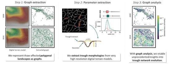
We used a three-tiered approach to represent the network of troughs as a graph and to extract morphological and environmental parameters from digital elevation models (DEMs). First, we built the graph from the underlying spatial data (
Graph Extraction), then we extracted the trough parameters (
Trough Parameter Extraction), and finally, from these results, we evaluated the graph with methods from graph theory (
Graph Analysis) (
Figure 2). We implemented the entire analysis with Python and partly relied on imported libraries for certain functions. These module dependencies for each sub-step are noted in the workflow diagram in
Figure 2.
As we aim to provide an approach for analyzing these kind of thaw-affected ice-wedge polygonal landscapes at pan-Arctic scales, we used methods that allow generalization and scaling to large areas and require only little user interaction. We further focused on algorithms with low computational complexity to allow scaling of the approach to extensive study areas. The algorithmic complexity of each step in the workflow is also shown in
Figure 2.
3.1. Materials
The extraction of a graph representing the network of ice-wedge troughs requires DEMs with high spatial resolution. In this study, we used DTMs generated from LiDAR point clouds which were acquired in 2009 and in 2019 in the same study area. The first dataset was acquired between 27 June and 2 July 2009 with an Optech ALTM 3100 LiDAR system at flight altitudes of 1000
. The average point density was 2 points/
. We created DTMs from the point clouds with 1
spatial resolution using the Quick Terrain Modeler (QTM) v.8. The vertical accuracy of the DTMs was between
and
(further details on processing are described in Jones et al. [
23]). We used a full-waveform Riegl LMSQ-Q680i sensor to capture the second LiDAR dataset at flight altitudes around 500 m on 22 July 2019. Here, the average point density of the georeferenced point clouds was 5 points/
. The vertical accuracy of the resulting DTM with 1 m spatial resolution was better than
m. In order to obtain DTMs from the point clouds, we followed a three-step approach. First, we classified the multiple target waveforms in vegetation and bare ground returns using echo width, amplitude, and target counter given in the raw data product. Next, we post-processed all ground returns to form the georeferenced point cloud data referenced to WGS-84 and combined the X, Y, and Z coordinates of each laser point with the post-processed GNSS (global navigation satellite system) flight trajectory (PPP processing with Waypoint 8.4 software), INS data, lever arms and squint angle corrections. Prior to the final processing, we determined the squint angles using a semi-automatic cross-calibration over runway and hangar buildings. In the final step, we built the DTM using an inverse distance weighting interpolation scheme. In
Figure 1c,d, we show the topography of the study area for 2009 and 2019, respectively. The area under investigation in our study covers
of the intersecting datasets from the acquisitions of both years (see
Figure 1b).
3.2. Graph Extraction
In the first workflow step, we extract a graph that captures key elements of the ice-wedge trough network from the underlying DTM data. In detail, graph edges delineate the ice-wedge troughs and the graph nodes represent intersections of troughs between three or more polygons. The process of graph extraction directly provides information on the spatial location of the nodes and their connectivity to neighboring nodes based on the real-world network of ice-wedge troughs. While in conventional applications of graphs, Boolean logic determines the connectivity of two nodes (either they are connected or not), we go further by including the ‘pathway’ of the trough, as real-world troughs do not always connect two intersections by the direct and shortest distance. Graph edges therefore need to hold information on the direction, i.e., the spatial course in the XY-plane, of the ice-wedge trough, as well.
3.2.1. DTM Detrending
Since we focus in this study on microtopographic changes induced by ice-wedge trough degradation, we considered any overlying meso-scale regional topography irrelevant and removed it. We applied a spatial detrending procedure to the DTM in order to produce a new elevation model maintaining only micro-topographic structures of the area of interest (so-called ‘detrended DTM’,
Figure 3a). For this, we used a square uniform filter with edge length
to extract the regional topography trend and then subtracted it from the original DTM according to
To determine the best-fitting edge length c of the uniform filter, we minimized the mean squared error of local height differences between the original DTM and the detrended DTM. For this, we first rendered 100 detrended images, each with a different detrending filter edge length between zero and 100 . We then manually extracted point pairs at ten select locations, where the first point of each such pair was always within a trough, while the second, reference, point was located in the polygon, but in the direct vicinity of the first (point pairs where approximately 5 to 8 apart). We calculated the absolute height difference between each point of a pair for the DTM, as well as for each of the 100 microtopography height models. Ideally, the difference in Z-value between two points of a reference pair would be identical for the DTM and the perfectly detrended microtopographic result. For the underlying analysis, we determined an optimal filter edge length of 16 . The resulting detrended microtopographic image had a mean squared error of based on the investigated ten point pairs. Detrending with this approach requires an algorithmic complexity of , with p being the number of pixels in the DTM.
3.2.2. Binarization and Denoising
We achieved a binarization of the detrended microtopography DTM (
Figure 3b–d) by adaptive thresholding [
46,
53] that segmented the image into pixels that belong to a trough and those that do not belong to a trough. The computational complexity for the binarization step lies at
, with
p again representing the number of pixels in the DTM.
The resulting image of the binary segmentation was affected by impulse noise (salt-noise), which corresponds to a number of false positives for the classification of trough pixels. In order to eliminate this noise, we removed any pixel clusters characterized as
troughs that were smaller than 15
from the segmentation. To further clean the image segmentation from persistent noise, we performed morphological closing by one pixel on the foreground class of
troughs. Morphological closing on a binary image corresponds to the operation of a morphological dilation followed by morphological erosion [
54]. Since erosion cannot disconnect a pixel cluster into multiple subclusters, as the minimum cluster width will always remain one pixel, separate clusters that were initially connected during the dilation process remained connected. These morphological procedures ensured that even weakly segmented troughs were treated as continuous from one trough intersection to the other.
3.2.3. Skeletonization
Once we had the image binarized and cleaned from noise, we computed the skeleton of the class
troughs (
Figure 3e). Skeletonization is also a concept from digital image processing that aims to reduce the foreground class to one-pixel-wide representations, while preserving the topology of these foreground features [
54]. The implemented function was based on Lee et al. [
55]’s version of the algorithm and also operates with a complexity
. Lastly, we again removed any skeleton pixel clusters with too few pixels (<15) in order to minimize faulty segmentation and therefore reduce noise.
3.2.4. Transformation to Graph
In the skeletonized image, every skeleton pixel now had one to eight neighboring skeleton pixels (we allowed 8-connectivity and thus included vertically, horizontally, and diagonally neighboring pixels). Only if the trough pixel in question exhibited exactly two neighboring trough-skeleton pixels, we considered it part of an edge. Skeleton pixels with one or three and more neighboring skeleton pixels were considered as nodes, since these are the channel intersections or endpoints within the trough network. For each node, we stored the pixel coordinates of the intersection as parameter to the nodes. The edges of the graph do not just connect two spatially fixed nodes along the shortest path but they follow the path of the trough between these nodes. Since polygon borders did not always run in an exactly straight line, but were partly bent, the length of a trough can be greater than the shortest distance between two intersections. The corresponding underlying pixel coordinates, along with the actual trough length which corresponds to the distance that water has to potentially travel in the trough, was stored as edge weights in the graph. Converting the pixel-based skeleton to a graph is computationally rather efficient and scales with the number of skeleton pixels. As this number is linearly dependent on the number of overall image pixels p, the computational complexity is as well.
In graph theory, the direction of an edge is defined by the ordered pair of nodes, where the first node of a pair defines the starting node of an edge, and the second node of a pair defines the end point. For each graph edge, we determined the absolute elevation above sea level of the two adjacent nodes from the original DTM and defined the hydrological flow direction to lead from the higher to the lower lying intersection. Such graphs with a clearly defined edge direction are also called digraphs [
56]. The operation of determining the direction of flow scales with
,
e corresponding to the number of graph edges. Given that according to the laws of gravity, under normal circumstances, water will not flow upward, the extracted graph must also be acyclic. However, cyclicity (loops) may exist in the case of two directly connected nodes
u and
v. This phenomenon occurred when both neighboring nodes featured the exact same height. In these cases, the algorithm for determining the flow direction recorded an edge that flowed from
u to
v and a second edge that flowed from
v to
u. It is most likely that the trough intersections underlying the nodes
u and
v in question were water-filled and therefore had the same elevation information in the DTM.
3.3. Trough Parameter Extraction
In order to extract morphological information on ice-wedge troughs in a thaw-affected landscape, we further analyzed the troughs individually. As single troughs can exhibit varying depths and widths over even short distances, we sectioned the troughs into segments of 1 length and determined depth and width for each one-meter segment individually. This corresponded to the spatial resolution of the image and therefore the greatest possible detail. The computation for all subsequent steps required for the extraction of trough parameters is dependent on the number of edges in the extracted graph e and scales linearly with .
3.3.1. Transect Partitioning
We defined a transect as being a cross-section of the skeletonized trough at a given skeleton pixel
p. A transect is roughly perpendicular to the path
in
p;
, and
being the neighboring upslope and downslope pixels in the trough’s skeleton, respectively. Based on the skeleton image of the troughs, for each trough of pixel length
x, we extracted a total of
transects. We did not consider the first and the last pixel of a trough due to their proximity to an intersection, as trough width and depth would be affected by the intersection configuration. Considering the neighboring two pixels of the skeleton, as well as the 8-connectivity of the skeleton and the flow directionality, there existed five possible rotation-symmetrically variant layouts for the arrangement of the trough skeleton pixels
,
p, and
.
Figure 4 depicts these five scenarios. Scenarios in
Figure 4a–c represent cases for which the extracted transect is truly perpendicular to the tangent of
s in
p. The transects for cases
d and
e are only approximations to the perpendicular. The true perpendiculars to the tangents of
s in
p would cut pixels at unequal lengths, which would unnecessarily complicate computation. We therefore compromised with horizontal and vertical transects for cases
d and
e and all their rotation-symmetrically equivalent settings.
The length
of a transect measured in pixels, corresponding to the length of the red line in
Figure 4, can be of arbitrary size. The true transect length
depends on the length in pixels
, as well as the spatial resolution
r of the imagery. For diagonal transects (scenario
c), transect pixels are cut diagonally and therefore result in greater
. The relationship between
and
according to the spatial image resolution and the transect type is described by
To gain meaningful results, the true length of a transect needs to be greater than the expected maximum width of troughs in the analyzed landscape. It is sufficient to approximate this parameter by educated guess and for this analysis, we used transect lengths of 9 . This value is greater than the expected maximum width of individual troughs, but sufficiently small as to not regularly include neighboring troughs or other artefacts in individual transects.
3.3.2. Transect Parameter Evaluation
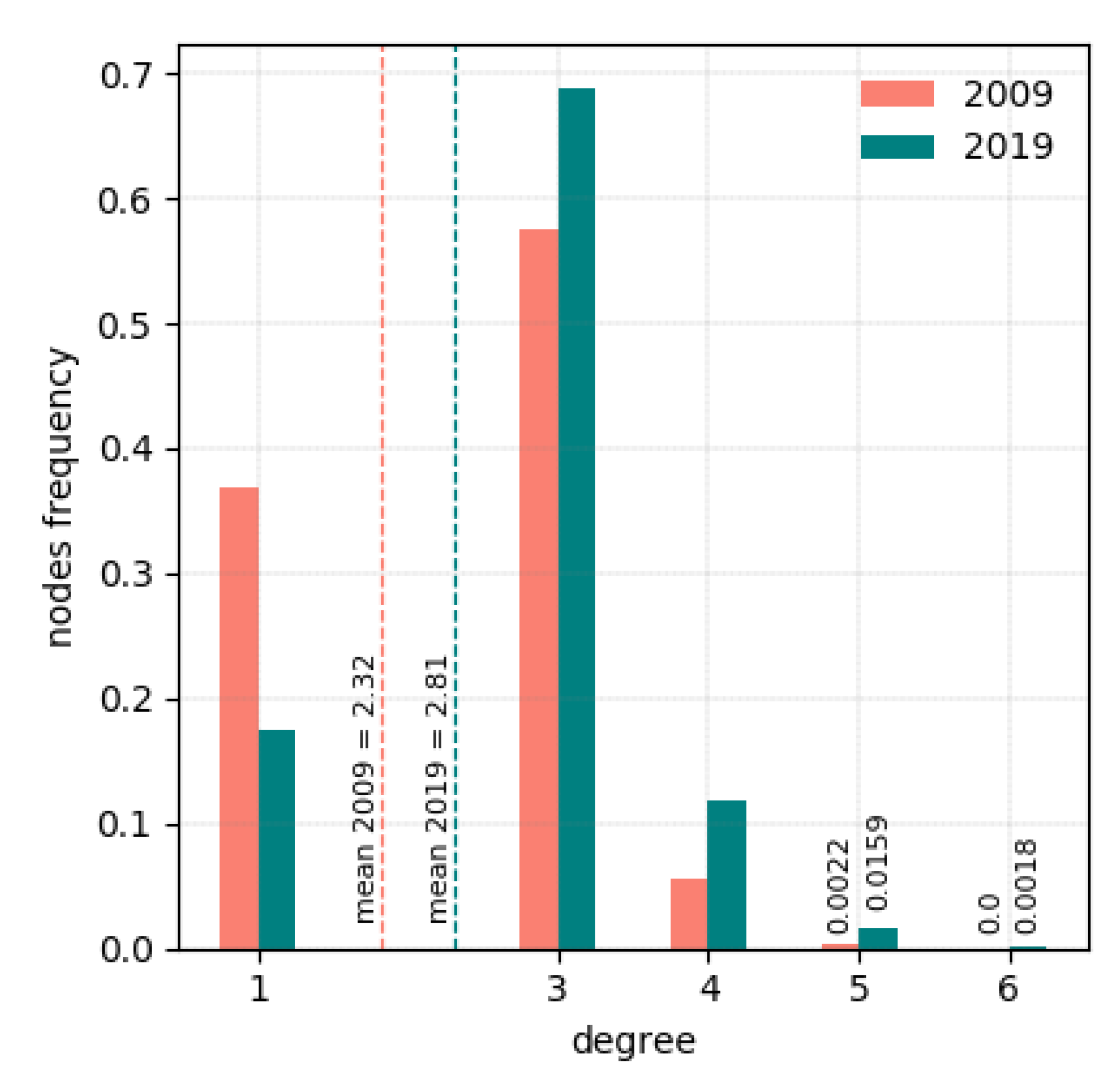
It can be an arbitrary decision to determine the width of a trough - even in terrestrial surveying - since trough borders usually gently slope into the trough bases, rather than showing clear-cut transitions and an explicit distance from one wall to the other. A similar challenge arises when measuring the depth of a trough. While the deepest point of the trough is clearly defined, the upper edge strongly depends on the trough’s shape. In order to approximate the trough width and depth, we fit a Gaussian function to the extracted profiles. The maximum and the full-width-at-half-maximum (FWHM) of the fitted function serve as a statistical measure of the trough depth and width, respectively.
Here we applied a non-linear least-squares fitting routine. The Gaussian function is defined by
with
denoting the mean and
denoting the standard deviation of the distribution. We initially assumed
to be equivalent to the index of the minimum value of the given transect. For the computation, we further set a minimum and a maximum value of 0.01 and 8.5 for
to adopt. This would ensure that the FWHM, serving as proxy for trough width, would only be able to range between ≈0 m and ≈20 m. We allowed the algorithm up to 500,000 iterations for fitting each trough. While this sub-step generally scales with
, the curve fitting per se was rather computing-intensive. Providing bounds for
already sped up computation by >300%. Further, since the Gaussian fit of every transect was entirely independent of any other transects, this step was easily parallelizable. We used multiprocessing to distribute curve-fitting of transects from different edges to multiple cores of the central processing unit (CPU). Therefore, the maximum number of possible parallel processes can be equivalent to the number of edges within the graph. However, in practice it is limited by the number of available cores and CPUs within the computing architecture.
We then evaluated all trough widths and depths along transects and computed the mean value of both parameters for each trough. We subsequently considered these mean values as overall trough widths and depths and added them to the graph as edge weights.
3.4. Graph Analysis
In the final step of the analysis we evaluated the graph metrics to gather detailed insights into the structure of the polygonal network and its hydrological implications, as well as to determine the progression of ice-wedge degradation within this landscape over time.
3.4.1. Number of Edges and Nodes
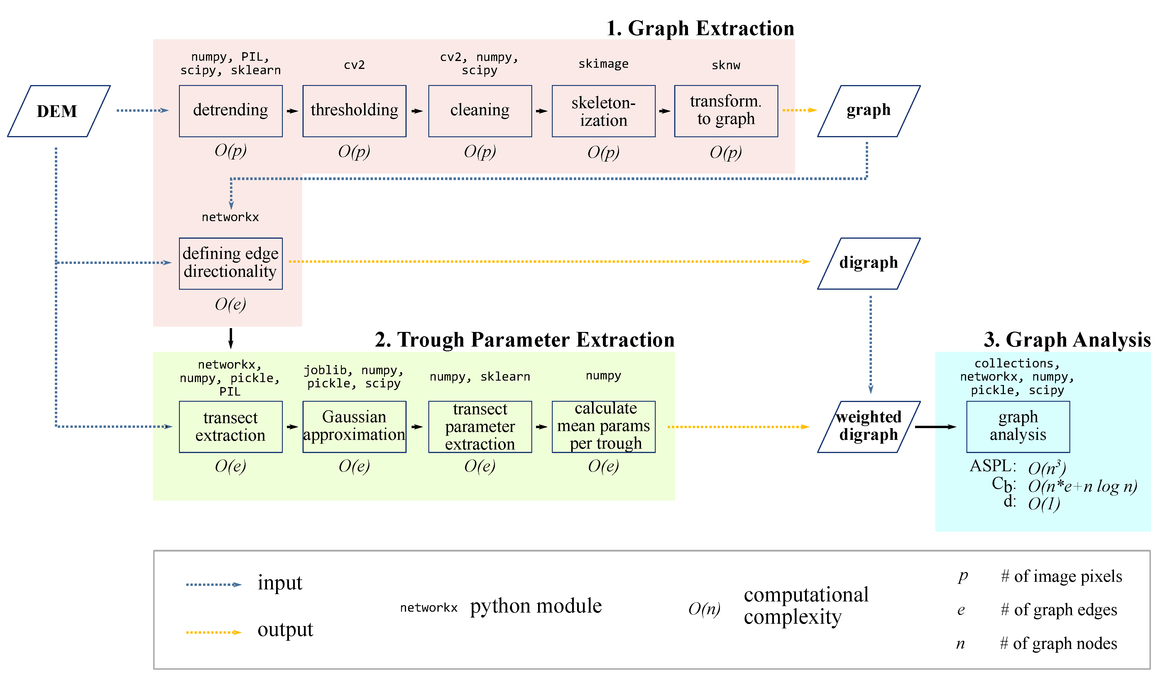
By analyzing the number of edges and nodes, we achieved a first overview of the size of our graph. With the underlying real-world trough network in mind, these values represented the number of troughs and trough intersections in the analyzed landscape. The parameter of node degree, which corresponds to the number of edges incident to a node further allowed us to estimate the complexity of connectivity within a network.
Nodes at the end of edges that represent dead-end troughs (troughs that do not connect to another trough at an intersection) only have one edge exiting or entering this node. Dead-end troughs do not contribute to the hydrological connectivity of a landscape, and a large number of such dead-end troughs will lower the edge-to-node ratio for a graph, which is an indicator for a thaw-affected landscape in transition. It was further possible to identify single troughs or even larger regions within the hydrological network that are more likely to inundate. Nodes that only register incoming edges and therefore represent sinks defined these areas. Given insufficient ground infiltration, we expected areas around sink nodes to exhibit ponding, as any water flowing through the network would accumulate here. Source nodes, on the other hand, only featured outgoing edges and we expected them in areas of rather drier soils.
3.4.2. Average Shortest Path Length
The average shortest path length (ASPL) within a network denotes the average distance to pass when traveling along the shortest path between two nodes for all possible pairs of nodes within a graph. It is a measure of transportation efficiency in a network [
57]. We acknowledge that in a hydrological context, water does not necessarily follow the shortest path. However, for very flat landscapes such as in this study region, we can work with this assumption as a first-order approximation to flow behavior. For our trough network, a shorter ASPL signified shorter flow distances for water in the troughs. Assuming that flowing water in troughs promotes sediment erosion of the trough walls, longer ASPLs suggest longer drainage pathways subject to erosion [
40]. For measuring the ASPL, the directionality of the graph’s edges was important, as water will only flow unidirectionally along the downwards gradient of the landscape within a trough. For directed graphs, we calculated the average shortest path length with
with
V being the set of nodes within the graph
G,
being the shortest path from nodes
s to
t, and
n being the total number of nodes in
G. For the calculation of the distance, we have taken the fact that troughs do not always follow a straight line between two nodes into account. The determination of all shortest paths between any two nodes within the network scales with
,
n corresponding to the number of nodes [
57].
3.4.3. Betweenness Centrality
The betweenness centrality in graph analysis is a measure of
centrality or importance of individual edges within a network. For each edge, it calculates the number of shortest paths between any two vertices that pass through the edge in question. The corresponding Equation (
5) is based on Brandes’ [
58] implementation and follows
with
being the number of shortest paths and
being the number of shortest paths passing through node
v, with
and
. It scales with
.
An edge with a higher betweenness centrality value is likely more important to ensuring hydrological flow in the network than one with with a lower value. In our application, this measure was useful for detecting nodes that connect two otherwise disparate parts of the trough network and thus helped us to characterize the likely areas of hydrological drainage of a region. For purposes of simplification, we assumed that we have equal water availability at each point and that the water flow does in fact follow the shortest path and not the steepest downslope path (see
Section 3.4.2). We also expected edges with higher betweenness centralities to experience larger water discharge [
40], which in turn may indicate a greater potential for further trough erosion.
3.4.4. Network Density
Network density is a measure that allows quantification of the network flow effectiveness within a network. It compares the number of existent edges within a graph to the number of potential edges given the number of nodes present. The number of potential edges
depends on the total number of nodes
n. In graph theory,
(potential edges in theory) is commonly considered to equal
In spatially explicit networks, Delauney triangulation and the Euler characteristic determine the number of total possible edges
(number of edges without them intersecting) and therefore corresponds to
. However, as Cresto-Aleina et al. [
59] have shown, it is possible to construct a hypothetical polygonal tundra with Voronoi diagrams, thus approximating
[
60] via
We then calculated network density
d with
with
being the number of actually existing edges within the analyzed graph. When analyzing a time series with
k graphs
, it is likely that at different time steps, the graphs have a differing number of nodes. It was therefore necessary to analyze the normalized network density to make the measure comparable over the time series. For this, we determined the number of potential edges
via Equation (
7) from the graph
with the largest number of nodes
n. The number of existing edges
will naturally remain dependent on
.
5. Discussion
5.1. Graph Extraction
With the approach described in
Section 3.2, we can successfully identify the general topology of the ice-wedge trough network from high-resolution LiDAR DTMs (see
Figure A1). While intermediate results from the workflow to some degree can introduce noise (e.g., during detrending and thresholding), we can handle such errors through, e.g., removing small clusters that are assumed to be false positive detections, and thus minimize the propagation of such errors throughout the workflow. As this step of graph extraction from elevation information is merely part of the pre-processing to prepare the data for the graph analysis, other methods of trough delineation such as from VHR satellite or aerial imagery might also subsitute this section of the highly modular workflow. Abolt et al. [
61], Zhang et al. [
62], Witharana et al. [
63] and Bhuiyan et al. [
64] have developed methods for segmentation of ice-wedge polygons in thermokarst-affected landscapes based on elevation models and multispectral imagery. Adapting their delineation results towards representation as trough skeletons, it would be possible to integrate the results into the next steps of the workflow described here, which underlines the versatility and adaptability of this conceptual study to always match the user’s need and the current state of the art. For simplicity and interpretability, we here chose to segment the DTMs using algorithms from traditional computer vision, such as thresholding and morphological image analysis (dilation, erosion, skeletonization) rather than deep learning algorithms [
61,
62,
64]. With this approach, we do rely on certain algorithmic parameters that need to be determined by the user, such as the detrending filter radii, the extent of the morphological closing (number of pixels to dilate/erode), and the size of pixel clusters to eliminate. However, since we do not need to extract the exact centerline of polygon borders, but need only to approximate their locations, we allow for a certain range of freedom when determining optimal parameters. Graph representation, as opposed to raster images, provides a higher ratio of information content to data requirement. The ice-wedge networks from this study represented as graphs merely required one-fourth of the storage space that DTMs required [
65]. Further, this semi-automatic approach has significant temporal advantage for mapping polygonal landscapes over some previously conducted studies for which authors entirely relied on manual delineation [
66,
67] and which therefore do not scale well at all. In its current form, the workflow for extracting graphs from DTMs is highly suitable for representing the network of troughs in thaw-affected polygonal landscapes and therefore for utilization in the further processing and analysis steps also for larger spatial domains.
However, this intention is currently limited by the lack of comprehensive LiDAR data coverage and the difficulty of scaling such aerial surveys to entire polar regions. It is possible to generate VHR DEMs from space-borne and drone-based optical imagery using digital photogrammetric methods, which represents a more cost-efficient database than airborne LiDAR sensors do [
68]. The growing availability and continuously increasing spatial resolution of such VHR optical satellite imagery would further facilitate this trend. However, stereophotogrammetrically derived elevation models cannot yet adequately capture height information of the ground, but rather represent the surface elevation only. In tundra regions, where we expect dense grass coverage and shrubby vegetation, LiDAR-derived models therefore still represent the most confident approach to capturing adequate ground elevation information, which is necessary for analyzing polygonal trough morphology.
5.2. Parameter Extraction
The extraction of trough transects and the subsequent approximation of their elevation profiles through Gaussian functions renders results in line with previously observed morphologies: In Adventdalen, Svalbard, Norway, Ulrich et al. [
66] observed trough widths between
and
and depths ranging from
to more than 1
, with an average of
. For a study site on Ellesmere Island, Canada, widths ranging from 2
to 11
and depths between
and 1
were observed [
69]. While these numbers correspond to largely undisturbed ice-wedge terrain, Jones et al. [
70] further reported on microrelief associated with ice-wedge troughs in fire scars also located in North Slope, Alaska. Here, the authors observed relief differences of
m to
m at four different fire sites. Troughs at the unburned, upland control sites only measured depths up to
m.
In this study, the high accuracies reached in fitting the trough profiles indicate that Gaussian functions (mirrored along the horizontal axis) can accurately describe such profiles. In total, only 1.22% of troughs were approximated with
in 2009, 1.01% in 2019. These belong to transects that were erroneously extracted from the elevation model. Possible causes include unfavorable courses of skeleton pixels with respect to the underlying true troughs; i.e., the skeleton pixels
, as seen in
Figure 4, were badly positioned, which resulted in the respective transects being aligned along the trough instead of perpendicular to it. This would extract mostly flat transect profiles, which makes fitting an appropriate Gaussian curve difficult to impossible.
Examining the extracted parameters, we observed rather shallow, but nevertheless mostly well-defined, troughs throughout the study area for both dates. We found a general trend of widening troughs over the observed study period of ten years, however, the average trough depth has decreased in the study area. While we generally expect any thaw to progress both in the horizontal as well as in the vertical direction, the data suggest only a vertical progression. However, we must consider that the number of troughs has also increased in this time frame. This process introduces a large number of shallow channels in the initial stages of degradation, which lowers the average depth of troughs in the network. The formation of new troughs in affected areas post-disturbance in general, and in the ARF scar in particular, has previously been observed by Jones et al. [
23].
It is further important to note the discrepancy between the acquisition dates of the two DTMs (early July in 2009 and late July in 2019). Seasonal frost-heave and -settlement have been observed by Antonova et al. [
71], Liu and Larson [
72] and Iwahana et al. [
73], who report up to
of thaw settlement over entire landscapes, and up to
subsidence above ice-wedge troughs over the course of a season. This may influence the measured depths of troughs over the intra-annual time difference. However, since we generally observe an average trend towards shallower troughs, and the acquisition dates of the year are only three weeks apart, we can assume an only minor influence on our results.
Some very large width values (>10 m) were not in line with common trough widths observed at other locations [
66,
69]. We can likely attribute them to unfavorably positioned transects and therefore unrealistic transect profiles, or transect profiles that did not cross-section a real-world trough. We however excluded most of these from the further analysis by filtering for trough fits of
. We thus conclude that the FWHM functions as an adequate proxy to describing trough widths in thaw-affected polygonal landscapes.
A certain robustness of parameter estimation for ponded troughs is a further advantage of approximating the trough geomorphology with a Gaussian curve. As LiDAR measurements cannot penetrate the surface of water, resulting DTMs capture the elevation information of the water surface rather than the elevation of the underlying ground. For trough transects, this results in flattened height profiles, shadowing the true morphology of the trough underneath the water surface. Based on the sloping trough walls, we used the Gaussian function to reconstruct the continuation of the trough geomorphology below the water surface. However, we acknowledge that this morphology reconstruction can only adequately function for troughs with low water levels. The deeper the ponds within the troughs are and the larger their extent is, the greater the uncertainty of the below morphology and the lower the coefficient of determination of the fitted Gaussian will be. Sobek et al. [
74], Heathcote et al. [
75] and Messager et al. [
76] followed similar approaches by incorporating terrain slopes surrounding lakes into linear and non-linear models to predict their bathymetry.
Despite the specified limitations, fitting a Gaussian function (with only the two parameters and to approximate) to evenly spaced elevation profiles along thermokarst troughs provides an adequate method to estimate geomorphological parameters such as depth and width of the troughs. To date, and to the best of our knowledge, no alternative approaches have been published that are able to estimate these parameters from remotely sensed data, or in an automated fashion. While the described workflow is computationally expensive and the number of transects to approximate scales linearly with the area under investigation, the algorithm is highly parallelizable. The approach therefore scales well to potential pan-Arctic analyses.
5.3. Graph Analysis
Evaluating the extracted graph characteristics, especially under consideration of the edge’s weights (i.e., the trough’s parameters), we observe a rather diverse thermokarst landscape in transition. For the study site covering an area of 630,000 m
, we extracted 54 isolated components, which corresponds to 54 individual trough networks that were hydrologically not connected in 2009. The majority of these non-connected components featuring only few nodes and edges, however, represent single troughs that presumably have only recently formed. Since we have observed considerably fewer isolated components in 2019 (six components), we infer an ongoing process of ice-wedge melt and thermokarst development, during which the many individual components became connected to fewer, larger components through the development of new troughs. Generally, the presence of multiple isolated components also implies that not the entire landscape will drain (surficial drainage) once a single trough degrades into a nearby lake or terrain depression. Drainage would only affect troughs belonging to the same component as the drainage-inducing trough. The overall number of components thus provides an important measure for assessing hydrological connectivity in polygonal landscapes [
11]. The landscape in 2009 was therefore far less likely to drain entirely than the same landscape observed ten years later, indicating that this particular area is becoming more connected and prone to rapid drainage and possibly subsequent drying. It has been discussed that drained ice-wedge troughs promote the stabilization of ice melt and therefore decelerate further thermokarst development [
11].
In 2009, we observed 327 nodes that connect only to a single edge, corresponding to 36.78% of all edges within the analyzed network. In 2019, we counted 296 dead-end troughs in total (17.42% of all troughs). On the one hand, the high fractions of dead-end troughs underline the fact that the area is still in transition of the degradation process and that the process has not yet revealed troughs above all ice wedges along the polygon borders. On the other hand however, we are currently investigating only an arbitrary subset of an area strongly affected by ice-wedge thermokarst and therefore have artificially created a high number of dead-ends at the borders of the image subset. The latter reasoning is especially relevant for explaining the high number of dead-ends observed in 2019, where the polygonal trough network expands throughout the entire study area up to the image borders. This is not yet the case for the network observed in 2009, although, we do in some border regions observe artificial dead-end creation through cut-off troughs (especially in the northern and south-eastern area).
The betweenness centrality correlates negatively with the location of nodes at highest and lowest elevations within the study area. As detailed above, we generally observed higher betweenness centrality measures at intermediate elevations. Edges with the highest betweenness centralities represented those that are most important in connecting two almost disparate components of the network. They therefore play a major role with regards to the hydrological connectivity within a network. Since high centralities infer more surface water flow through the equivalent troughs (assuming uniformly distributed water availability), we can suppose a stronger hydrological erosion of the wedge ice and sediment and therefore increased trough depths and/or widths than within troughs of lower betweenness centrality values. Troughs with high centrality measures that are rather shallow and narrow are likely to have formed only recently, since these characteristics imply an only recently made connection between two subnetworks.
The normalized network density of 0.409 in 2009 implies that not even half of all potential troughs—assuming the ice-wedge network can be approximated by Voronoi cells [
35]—have become visible at the surface so far. Compared to the network density of 0.928 in 2019, we observed a strong increase in connections and therefore a multitude of new pathways for surface water to flow and drain within the observed area.
Throughout the analysis, it is, however, necessary to be prudent when only evaluating spatial subsets of the continuous landscape. In this study, we only analyzed an arbitrary subset of the degrading ice-wedge polygonal landscape and thus condoned the truncation of polygons at the study area’s outer borders. This leads to somewhat skewed measures of connected components, network connectivity, path lengths, and centrality measures, resulting in possibly false interpretations of drainage patterns and other hydrological implications. In order to eliminate this boundary problem, and therefore to generate more accurate predictions, it would be necessary to analyze only self-contained polygonal landscapes or entire hydrological basins at once. It is further important to remember that the elevation information from the DTM has a vertical uncertainty of m. This potential elevation error may in some cases result in wrongly determined flow directions within troughs with very subtle elevation differences (as are common in lowland landscapes).
In general, most methods from traditional graph analysis were developed for describing graphs that are spatially implicit (where edges can exist between any two nodes). In the geosciences, however, where spatial information is ubiquitous and represents a core aspect of the science, spatially explicit networks are more prevalent [
45]. Thus, graph analysis algorithms that can take the only few, local connections into account, or are at least robust towards such characteristics, represent important methods to describe our environment [
77]. As Keesstra et al. [
42] have discussed, especially the concept of network connectivity (temporal and/or spatial) has been gaining attention in the past years in the geoscientific context [
38,
39,
43,
65,
77]. While, to the best of our knowledge, no studies have described small-scale hydrological surface networks with graph-based metrics yet, Czuba and Foufoula-Georgiou [
39] have used similar approaches to examine connectivity within larger fluvial systems. In their study, the authors investigated the relationship between location and intensity of geomorphic change within a river network. They concluded that such graph-based frameworks are easily able to assess the impact of local-scale changes towards large-scale networks, thus underlining the usefulness and validity of analyzing connectivity measures in the context of polygonal ice-wedge landscapes as well. Marra et al. [
40] have further shown how betweenness centrality is an appropriate method to determine the importance of individual channels for water flow within a braided river stream system. This finding can be directly mapped to our application of identifying trough importance within our polygonal network in the Alaskan tundra.
6. Conclusions
With our approach at representing ice-wedge polygonal landscapes affected by permafrost thaw as graphs that we extracted from airborne LiDAR DTMs, we offer geomorphological and hydrological insights at unprecedented detail for changing Arctic tundra regions. The processing pipeline of extracting the graph as well as the morphological parameters of the trough network from digital elevation models presented in this study scales linearly with the study area size and is highly parallelizable. The methodology thus represents an important first step towards a large-scale analysis of thermokarst-affected landscapes throughout the entire Arctic. Especially in rapidly evolving environments, such as sites affected by disturbance events, the algorithm allows detailed monitoring of the erosional process in ice-wedge polygonal landscapes. For the study site of the Anaktuvuk River Fire scar in northern Alaska, we observed a considerable increase in the number of troughs, as well as their widening over the observed period of ten years. Simultaneously, the number of observed sub-networks in the study area has decreased as they have become connected to build fewer but larger hydrological drainage networks in the same area. In general, the structures and implications of the spatial graphs cannot only give insights to the area’s ecology and morphology, but provide valuable measures and parameters for further integration into numerical models of thermokarst degradation processes. The proposed representation of trough morphology with only two parameters especially facilitates this. In the context of network analysis, the research presented here provides further validation of the power and usefulness of graph-theoretic measures within the geo(-morphological) sciences. For permafrost research, however, this study presents an entirely novel approach towards quantifying surface dynamics in thaw-affected ice-wedge polygonal landscapes. As an almost fully automated approach relying on remotely sensed data, it thus establishes a promising framework for future larger-scale analyses of these vulnerable regions.


 ,
, 


