1. Introduction
The multipath effect refers to the phenomenon where signals from satellites arrive at the receiver antenna through multiple paths due to reflection and scattering. Both pseudorange and carrier phase measurements are affected by it. Theoretically, the maximum value of multipath on phase measurements can reach 1/4 of the wavelength [
1], so the influence should be considered when using global navigation satellite system (GNSS) technology to carry out high-precision data processing. In order to mitigate the multipath error, we can model it like some of the other errors in GNSS data processing. Sidereal filtering (SF) is a widely used multipath error mitigation method. Some scholars [
2,
3] have found that the multipath error could be separated and modeled by using the periodic repetition characteristics of the satellite orbit, and then the observations of the following days could be corrected and the multipath error will be mitigated. With the deepening of research, Seeber et al. found that the repetition period of te global positioning system (GPS) satellites is not a simple sidereal day, and there are also differences between different satellites [
4]. Ragheb et al. compared the methods of using SF based on the coordinate domain and the observation domain, and showed that the former is more computationally efficient while the latter can achieve better improvements [
5]. Compared with SF, the description of the multipath error in the space domain is also an effective solution to mitigate its influence. Cohen and Fuhrmann established the lookup table for the antenna [
6,
7], and Dong et al. proposed the error correction method to establish the multipath hemispherical map by using a common receiver clock for the multiple antennas [
8,
9].
In the past, multipath modeling methods have mainly focused on the GPS. However, with the gradual improvement of the BeiDou navigation satellite system (BDS), it has been a research focus in recent years, and many studies about its performance have been published. Ye et al. used the SF method to carry out multipath modeling research for the regional BeiDou navigation satellite system (BDS2), and pointed out that the orbit repeat periods of satellites from different constellations are different [
10]. The SF based on single-differenced residuals, which are mapped from double-differenced observation residuals, was used to mitigate the multipath error. Shi et al. pointed out that the above additional constraint for double-differenced residuals is not appropriate, and new errors will be mixed into the positioning results [
11]. They extended Dong’s method based on the multipath hemispherical map to mitigate the multipath error of BDS in the double-differenced observation domain and obtained some useful achievements. When separating the multipath error of different constellations in BDS, a stationary geostationary earth orbit (GEO) satellite should be selected as the reference satellite, which reduces the application scope of the method.
Besides BDS, the Galileo navigation satellite system in Europe is also developing rapidly [
12]. In addition, with the recovery of the Russian economy in recent years, the Global Navigation Satellite System (GLONASS) realized full constellation operation again in 2011. According to the official statistics of the International GNSS Service (IGS) Multi-GNSS Experiment (MGEX), more than 120 satellites of the four major navigation satellite systems have been operating normally in orbit as of the end of November 2020 [
13]. In order to solve the problem of the limited number of available satellites for a single navigation system in complex environments, the integration of multi-GNSS will be the development trend of GNSS high-precision data processing in the future. However, there is little research on the multipath error modeling for Galileo and GLONASS. At the same time, with the development of GNSS, the issue of compatibility and interoperability has gradually received attention. In order to ensure the possibility of interoperability among these GNSSs, observation signals with relatively similar frequencies have been set up [
14,
15]. It is expected that the GLONASS-KM satellites launched in 2025 will begin to broadcast an L1 (1575.42 MHz) signal, which will be consistent with L1C after GPS modernization, E1 of Galileo, and B1C of BDS3 [
16].
In summary, satellite navigation and positioning technology is in the development stage, where multiple navigation systems coexist, and there are observation signals of the same or similar frequencies between the different systems. Multipath error fusion modeling methods are essential for multi-GNSS data processing. SF is the most widely used and effective multipath error correction method at present. This method uses the periodic repetition of satellite orbit to model the multipath error in the coordinate domain or observation domain, which is mainly used for static observation platforms. Compared with the traditional constellation composed of Medium Earth orbit (MEO) satellites only, BDS consists of three kinds of satellites—MEO, GEO, and inclined geosynchronous orbit (IGSO). However the orbit repeat periods are still quite different for the satellites in the same MEO constellation [
17]. Different GNSSs need to be modeled independently when using SF, which is cumbersome and inefficient in application. In addition, the effect of multipath error on satellite signals in the same direction should theoretically be the same when using the same frequency observations of different navigation satellite systems for the same observation platform [
8]. However, the formation mechanism of the multipath error has not been fully considered in the SF method. Therefore, to avoid the above-mentioned disadvantages of the SF method, using observations of multiple GNSSs and constellations in the space domain can achieve the purpose of making full use of the modeling data to finely describe the multipath error sources.
Based on the existing SF method, we first evaluated the orbit repeat period of satellites from GPS, BDS, and Galileo in different periods, and then proposed a data processing scheme that is suitable for the above three GNSSs for SF. In addition, a comprehensive modeling method in the space domain, called the multi-point hemispherical grid model (MHGM) for multipath error sources, was modified considering the characteristics of multi-GNSS with the same or similar frequency observations. Afterward, we compared the performance of the modified MHGM method and the SF method from a multi-GNSS point of view. Finally, the established MHGM using the data of multi orbit periods was compared with that of only one orbit period to verify the improvement of the model accuracy.
2. Materials and Methods
As the multipath error is related to the observation environments within a certain range around the station, which is the observation platform where the GNSS antenna is located, and the multipath error cannot be eliminated or mitigated by differential technology, it has been a major error source that affects the accuracy and reliability of multi-GNSS data processing [
18]. The inter-frequency bias should be estimated for ambiguity resolution because the frequency division multiple access (FDMA) signal mode is adopted in GLONASS, which leads to the application limitation of GLONASS in high-precision data processing [
19]. In addition, there are only three GLONASS satellites broadcasting code division multiple access (CDMA) signals currently [
20]. So, the experimental analysis is limited to the other three systems.
2.1. Sidereal Filtering for Multi-GNSS Multipath Correction
In order to reduce the complexity of the algorithm, the orbit repeat period of the same type of satellites in the same system is generally averaged to obtain the overall optimal SF models. Among the existing GNSSs, MEO satellites are used in GPS, BDS, and Galileo. However, the orbit repeat period is different because of the difference of the orbit parameters. The orbit repeat period of the GPS satellite is about 1 day and the Galileo satellite is about 10 days. BDS has adopted a mixed constellation of GEO, IGSO, and MEO satellites. The orbit repeat period of the GEO and IGSO satellites is about 1 day, and that of the MEO satellite is about 7 days. Therefore, the independent orbit repeat periods need to be set for these three systems. The orbit repeat period
of the above systems can be calculated from the relevant parameters in the broadcast ephemeris and Kepler’s third law, as given [
21],
where
is the square root of the corresponding standard gravity parameters of each GNSS for Earth,
is the semi major axis of the satellite orbit, and
is the correction of the satellite angular velocity parameter.
is the number of orbital revolutions of the satellite in its orbit repeat period. The calculation results of
are relatively large. Generally, for the convenience of description and use,
is further expressed as the time shift
of the days corresponding to the orbit repetition period [
10,
22],
where
is the integer day corresponding to the satellite orbit repeat period, and the values of
and
for the different constellations in each system are listed in
Table 1.
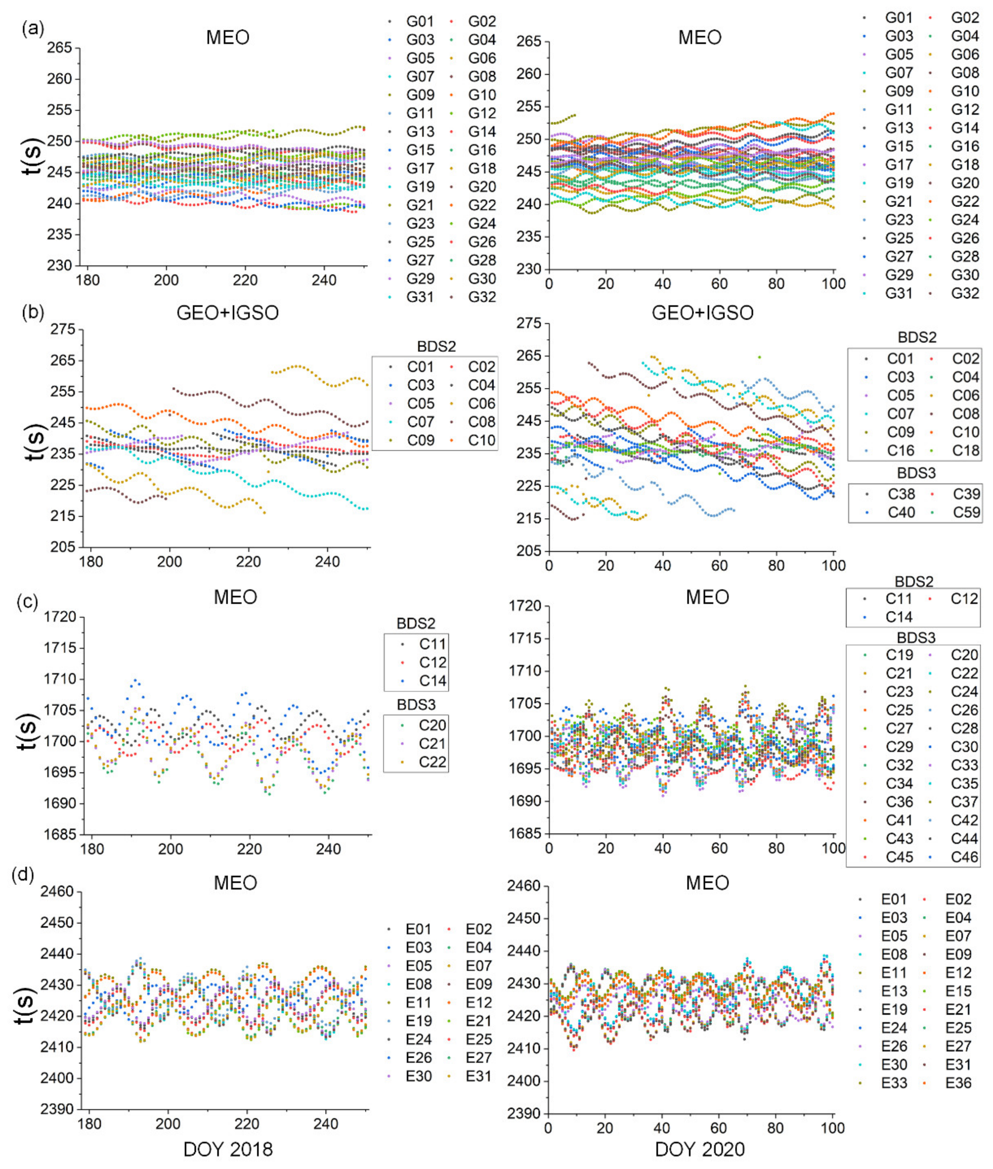
The time shifts of the orbit repeat period on days of year (DOY) 179~250 in 2018 and DOYs 1~100 in 2020 for each satellites were calculated. According to the statistical results of the time shifts of the orbit repeat period for different satellites in each system in
Figure 1, the orbit repeat periods of the different satellites with the same constellation type in the same system were relatively consistent. However, there were differences among satellites from same type of constellations in different systems. Taking the MEO satellites as an example, the time shifts of the orbit repeat period for GPS, BDS, and Galileo were still significantly different, so it was necessary to set the parameters for each system separately. The time shifts of the orbit repeat period for the satellites with the same constellation types were relatively stable in the long-term statistical results in
Figure 1. The time shifts of the GPS varied between 240 and 250 s. There were slight differences between all of the satellites, but the long-term changes of each satellite were relatively stable. The orbit repeat period of GPS was about 1 day, and the time shift was set as 245 s because of the statistical results of this kind of satellite; this parameter was as close as the result of 246 s obtained by Ragheb et al. using the autocorrelation of the station coordinate time-series [
5]. As shown in
Figure 1b, the corresponding shifts of the GEO and IGSO satellites of the BDS varied between 215 s and 265 s, and there was a gradual decreasing trend, but the time shifts increased with a jump at regular intervals. It was found that this was due to the orbital maneuver, and the parameter SatH1 could be found in the broadcast ephemeris [
23]. When the orbital maneuver phenomenon occurred, it changed from 0 to 1. In addition, the orbit repeat periods of the satellites with the same type of constellation from BDS2 and the global BeiDou navigation satellite system (BDS3) were basically the same, so the unified time shifts could be adopted in the multipath error correction of SF. The orbit repeat periods of the GEO and IGSO satellites of BDS was 1 day, and the time shift was set as 246 s, which is the average statistical results of such satellites. The orbit repeat period of MEO satellites was 7 days, and the time shift was set as 1700 s, which is the average statistical results of such BDS2 and BDS3 satellites. These were also consistent with the results calculated by Dai et al. using Kepler’s third law and broadcast ephemeris for different constellation types of BDS2 [
24]. There are few analyses related to the SF period of the Galileo in related research at present. Based on the above statistical method of GPS and BDS satellites, the orbit repeat period of Galileo satellites was 10 days, and the time shift of Galileo satellites was set as 2424 s, which is the average statistical results. According to the above analysis results of each GNSS, we further extended the SF method of the observation domain in Galileo, so as to realize the SF modeling of multi-GNSS.
2.2. Multi-Point Hemispherical Grid Model for Multi-GNSS Multipath Correction
If the receiver antenna was above an infinite plane and was only affected by a single reflected signal, the error caused by the multipath effect on the carrier phase observation can be described as follows [
25]:
where
is the height of the reflector from the antenna phase center,
is the incident angle of the reflected signal,
is the reflection coefficient of the reflective objects, and
is the wavelength of the satellite signal.
Assuming that the receiver antenna and the surrounding environment remain unchanged, the signals of the same wavelength were reflected and entered the receiver antenna from the same incident angle when the different satellites passed through the same position in the sky. According to (3), the multipath error of the carrier phase observations should be the same [
8]. From the frequency setting of each GNSS, it can be found that the frequency of the GPS carrier signal L1, Galileo carrier signal E1, and BDS carrier signal B1C was 1575.420 MHz, and B1 of BDS had a slight difference with the above frequency, which was 1561.098 MHz. Therefore, it is theoretically feasible to use the observations of multi-GNSS for integrated modeling of the multipath error.
Based on the above analysis on the frequencies of different GNSS signals, we established a multipath modeling method for multi-GNSS, and the precise description of multipath error sources in the environment around the station was realized in the space domain. The residuals of the double-differenced carrier phase observations in the ambiguity-fixed period were used as the input information. Then, a multi-point hemispherical grid model at each station was established and finally the model of each station could be obtained after the grid points of each model were parameterized and solved by the estimator [
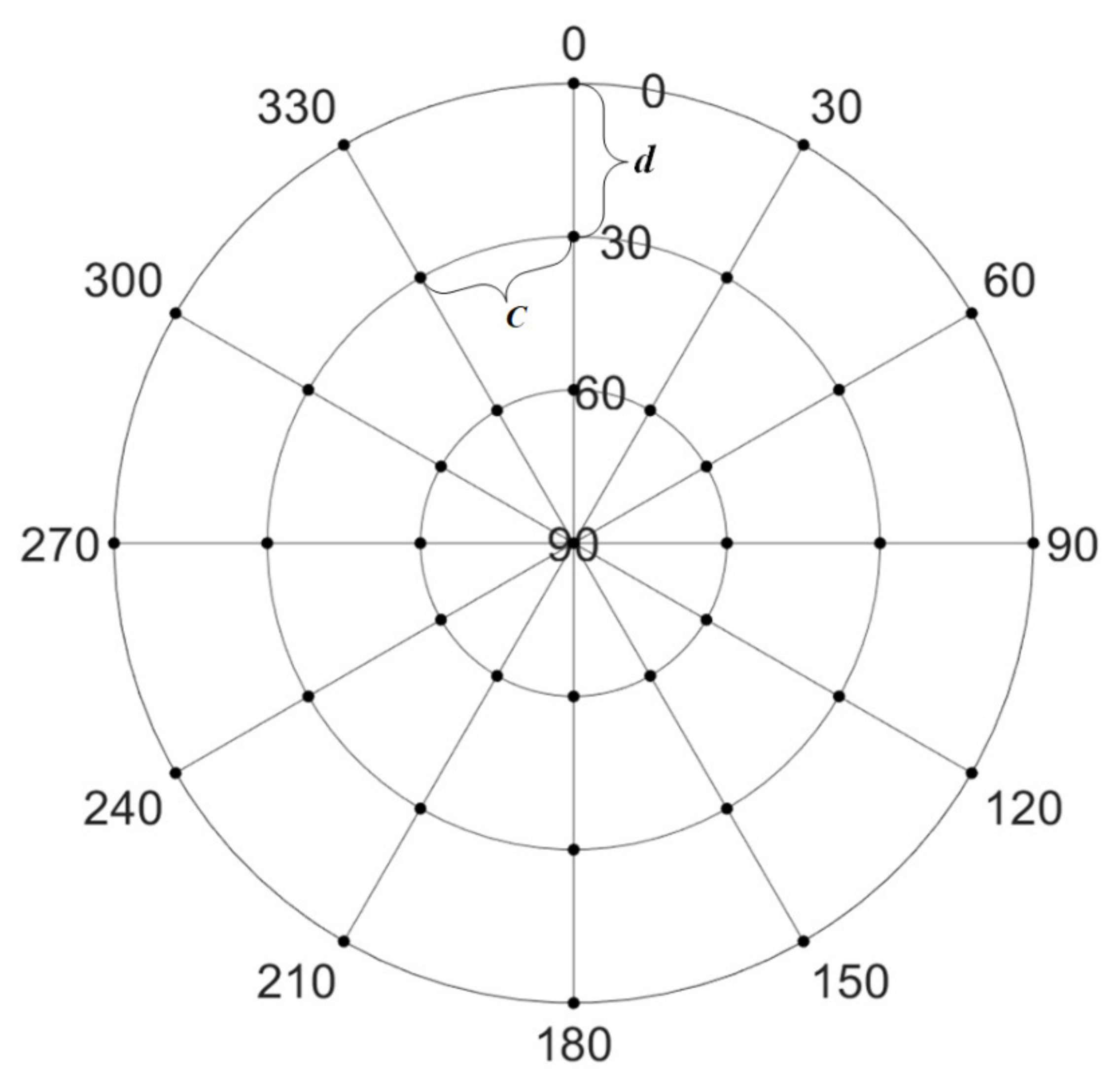
26]. First, the hemisphere was established with the antenna phase center of each station as the origin and was divided into grids according to the elevation angle and azimuth angle. The minimum value of the elevation angle was set as
, the maximum value was set to
, and the grid point parameter was set in the zenith direction. The interval of the hemisphere partition could be set as
and
, and the value of
and
determined the density of the grid partition. The smaller the partition interval, the more parameters to be estimated and the more computing resource consumption, but the higher the precision of the model.
Figure 2 shows an example of the grid partition for a hemisphere with
= 0°,
= 60°,
=
= 30°.
Given the double-differenced residuals
with ambiguity-fixed solutions between two stations
p and
p and two satellites
s and
t. The residual corresponding to satellite
on station
is
. Supposing the parameters of the four grid points involved in the grid point of the satellite are
,
,
and
, there is a case involving three grid point parameters when the elevation angle is greater than
. Then,
could be express by the parameters of the grid points, as follows [
26]:
where
is the interpolation coefficient obtained using a bilinear interpolation method when four grid points are involved [
27], and
can be obtained by using a trigonometric interpolation method when three grids are involved [
28,
29]. The residuals of each satellite on each station can be expressed using the grid point parameters involved, and the double-differenced residual
can be expressed as follows:
Then, the normal equation corresponding to the parameters of the grid points that need to be estimated can be constructed using (4) and (5). In addition, the theoretical maximum value of the multipath error is 1/4 cycle of the wavelength according to (3) for the grid point parameter
, so the following virtual observation equation can be added to each grid point parameter.
Because there is a certain correlation between the surrounding environment of the station corresponding to the adjacent grid point., if the grid point parameters
and
are adjacent to each other, the virtual observation equation can be added according to their correlation.
The above two kinds of virtual observation equations of (6) and (7) can further improve the accuracy and reliability of the modeling results. First, the double-differenced residuals with ambiguity-fixed solutions are added to the parameter solution and establish the observation equation according to the weight of the precision of the carrier phase. Then, the above two types of constraints for each grid point and neighboring grid points are added, which can be established according to the weight of 1/4 cycle of wavelength and empirical threshold of the multipath error between the grid points. Finally, the parameters of MHGM for each station are calculated as a whole in the estimator. Based on this principle, the established model is an integrated model for multi-GNSS, without considering the diversity of the different systems and constellations.
3. Results
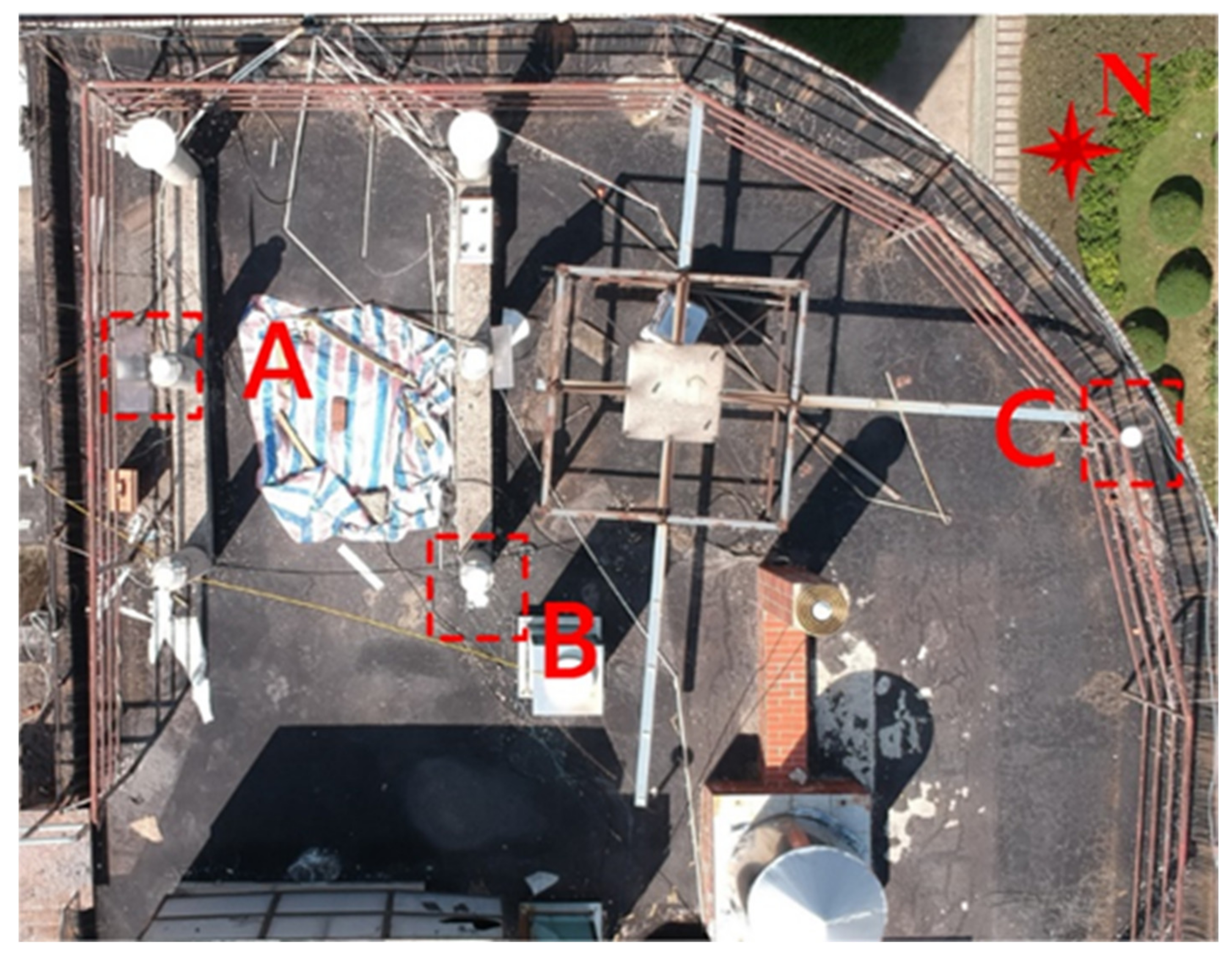
A set of data collected on the top floor of the Teaching and Experimental Building of Wuhan University on DOYs 215~234 in 2018, with a total of 20 days, was selected for testing and analysis. Three stations A, B, and C were set up during the collection of this set of data. A metal baffle was mounted in the west of station A to simulate a strong multipath environment, and stations B and C were normal. The distances between the three stations were 2.7 m, 4.7 m, and 6.9 m, respectively. The location relationship and surrounding observation environment are shown in
Figure 3.
The positioning and navigation data analyst (PANDA) software developed by Wuhan University was used for the data processing [
30,
31]. The specific strategies using in the data processing are shown in
Table 2.
In the process of modeling, the coordinates of the three stations were fixed to known values so as to obtain high-precision carrier phase residuals. Considering that orbit repeat periods of different satellites vary from 1 to 10 days, the observation data of DOYs 215~233 in 2018 were selected for the multipath error modeling. The observation data of DOYs 225~234 in 2018 were used for the validation analysis to evaluate the improvement of the observation residuals, positioning results, and other indicators after adopting different error correction strategies. For the MHGM, we set = 5°, = 85°, and = = 2° considering the usage of computational resources. The corresponding weights of (5), (6) and (7) were 5.0 mm, 4.8 cm, and 1.0 cm per degrees, respectively.
3.1. Use the Observations from Days of the Previous Orbit Repeat Period for Testing
According to the introduction in previous section, when using the observations of the previous orbit repeat period for SF, it is necessary to set their respective repeat periods for different constellation types of different GNSSs. At the same time, the same data are used for multipath error modeling and verification in order to compare the effectiveness of SF and MHGM.
Table 3 shows the double-differenced residuals of each GNSS with ambiguity-fixed solutions for the verification days, before and after multipath error correction.
In
Table 3, N represents the processing strategy without model correction, S refers to the processing strategy of correcting multipath error with the SF method, and M(1) refers to the strategy of correcting the multipath error by MHGM. The average RMSs of the double-differenced residuals were distinguished by GPS, BDS, and Galileo. The test results of the tenth-day show that the double-differenced residual after multipath error correction was significantly reduced compared with the uncorrected one. The average improvement rates of SF and MHGM were 49.6% and 53.7%, respectively.
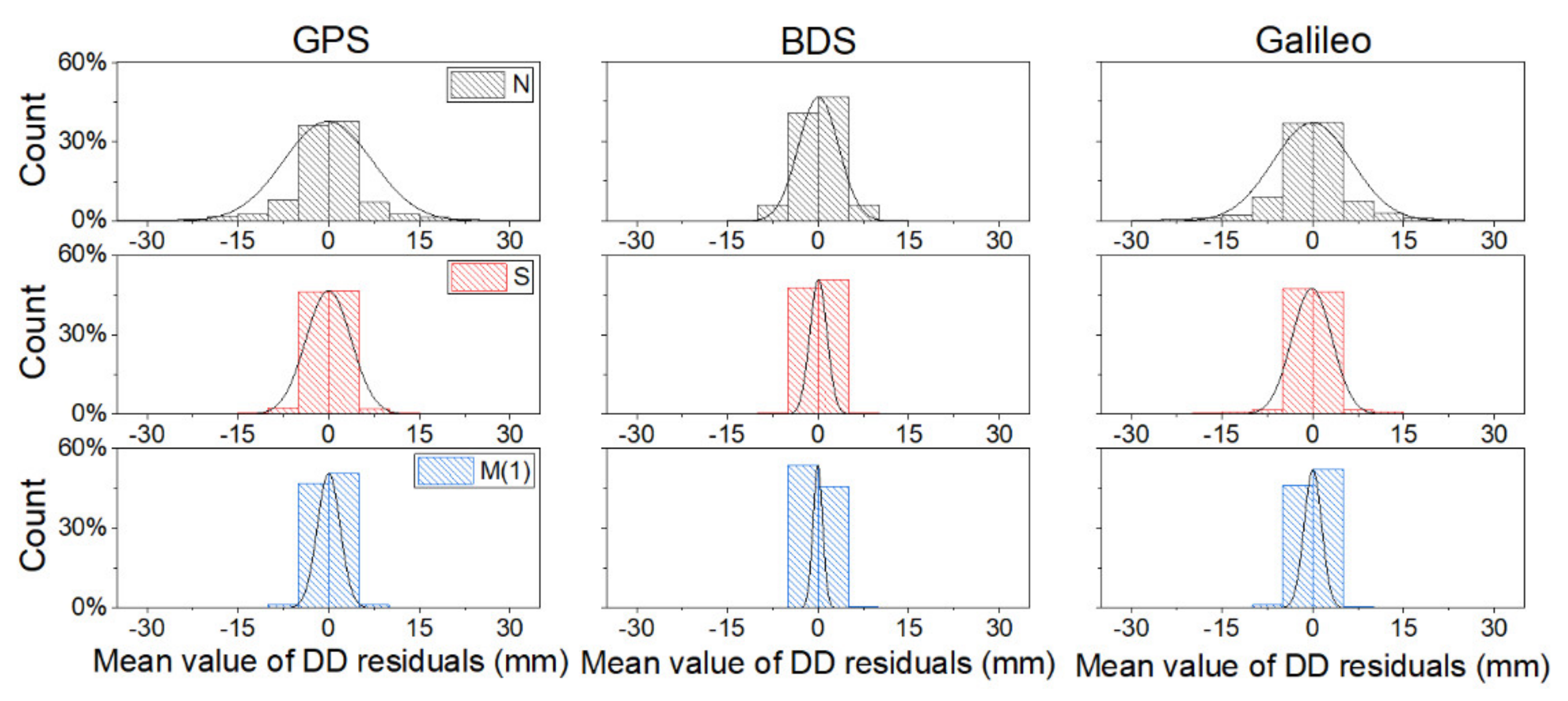
We also gathered the statistics on the average values of each double-differenced residuals in the ambiguity-fixed period for the ten-day verification data and fit a normal distribution of these residuals, so as to further reflect the change of carrier phase residuals before and after the multipath error correction. The results are shown in
Figure 4.
It can be seen from
Figure 4 that the distributions of the double-differenced residuals in N of each system are more scattered without multipath error correction and the data distribution of S and M are more centralized. Taking GPS as an example, only 37.5% of the uncorrected double-differenced residuals were distributed between ±2.5 mm. The percentage of data in the range of ±2.5 mm increased to 46.7% after the SF model correction, and 50.7% of the double-differenced residuals were concentrated in the range of ±2.5 mm after MHGM correction. The statistical results of BDS and Galileo were similar to these of GPS.
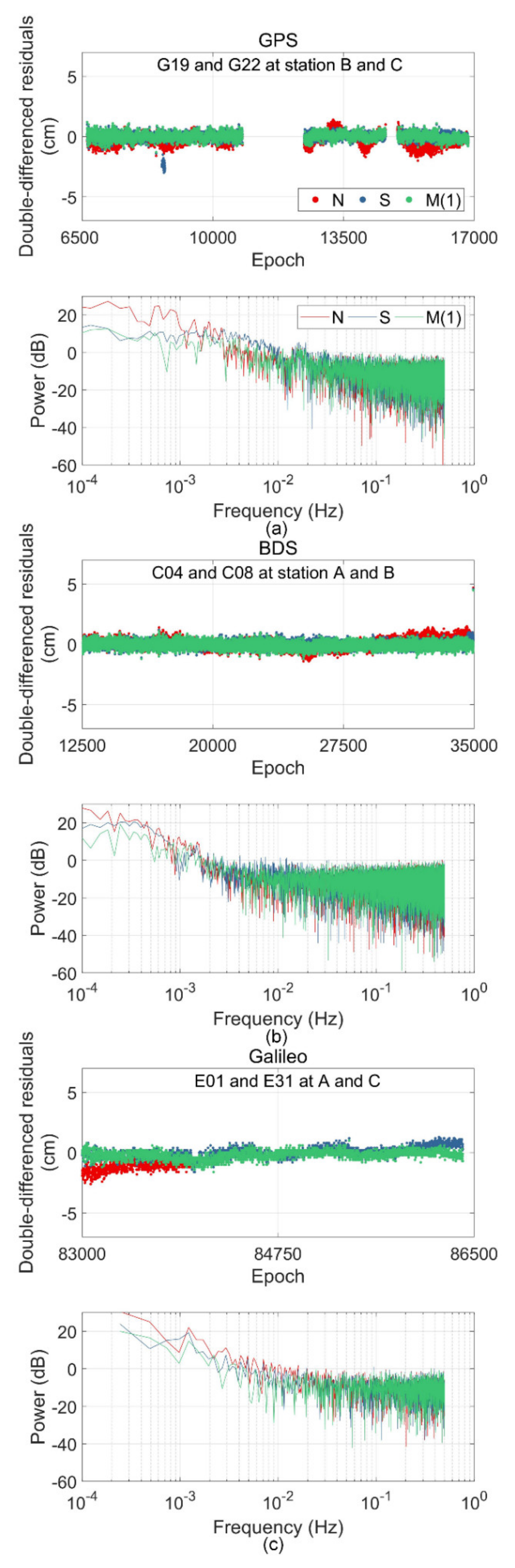
Multipath errors caused by different reflectors have different forms in the frequency domain. We also analyzed the changes of three groups of double-differenced residual sequences and signal power spectrum before and after multipath error correction under different systems. As shown in
Figure 5, the results of the power spectrum analysis prove that the two studied methods can effectively mitigate the low frequency multipath signal in the sequence. For a noise signal greater than 0.1 Hz, the correction of SF and MHGM was relatively consistent.
Compared with the observation residuals, the improvement of the multipath error correction on the positioning results may be more intuitive in practical application. Therefore, we also collected statistics on the positioning results for the verification days before and after correction with SF and MHGM methods. Station C was fixed and the coordinates of Stations A and B were solved according to the static relative positioning mode during the experiment. The observation time involved in the data processing was set to one hour and the positioning results for a total of 240 tests in 10 days were counted.
It can be seen from
Table 4 that the positioning accuracy after model correction was better than that without model correction. For Station A with baffle to simulate a strong multipath, the improvement of the positioning accuracy was more obvious. At the same time, the positioning accuracy after model correction with MHGM was slightly better than that of SF, and the results showed that the performance of MHGM and SF was comparable.
3.2. Use the Observations from Multi-Day for Testing
According to the experimental results in the previous section, MHGM and SF were comparable when using the observations from the days of the previous orbit repeat period. In this section of the experiment, we further used the observations of DOYs 215~233 in 2018 for multi-day modeling of the MHGM. Considering that Galileo had the longest orbit repeat period among the three systems involved in the solution, the duration for the multi-day modeling was set to 10 days. The start and end dates correspond to
Table 5. Meanwhile, the validation data should be consistent to analyze the improvement of the MHGM modeling results by increasing the amount of data involved in the modeling. The specific test plan is listed in
Table 6.
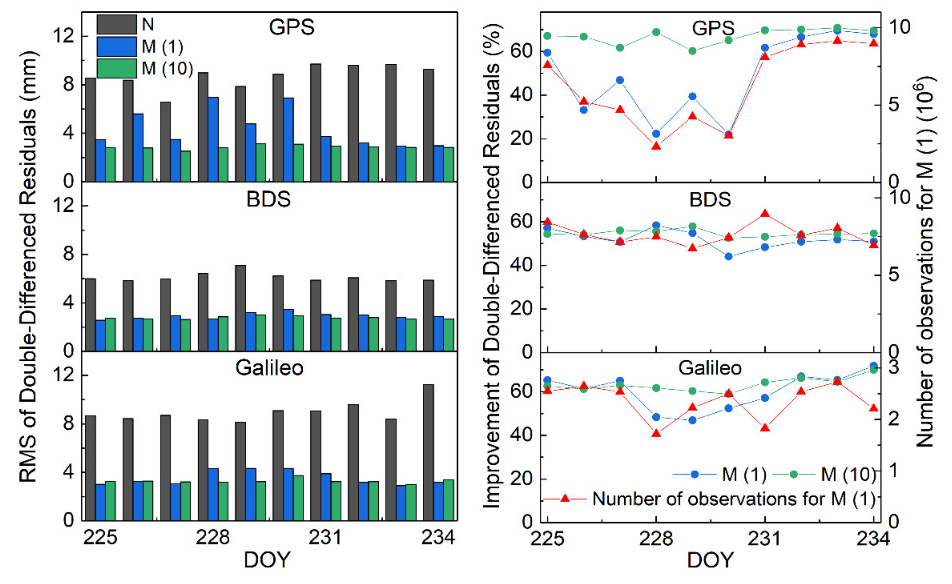
For the verification day, the mean RMS of the double-differenced residuals in the ambiguity-fixed period after multipath error correction was compared using the observations from days of the previous orbit repeat period and the multi-day for modeling MHGMs. The results are shown in
Figure 6.
In
Figure 6, N indicates the strategy without multipath correction, M (1) refers to the strategy of establishing MHGM for multipath error correction using the observations from days of the previous orbit repeat period, and M (10) is the strategy for establishing MHGM for multipath error correction using all ten-day observations. The left part of
Figure 6 shows the change of mean RMSs of double-differenced residuals for three strategies of N, M (1), and M (10). It can be seen from the figure that the RMS of the double-differenced residuals further decreased with multipath error correction strategy M (10). An average improvement of 13.1% in the RMS of the double-differenced residuals could be achieved compared with M (1). The statistical results of M (1) had a relatively low improvement over a few days compared with M (10), which was especially obvious in GPS. Therefore, the right part of
Figure 6 shows the change of RMS improvement of the double-differenced residuals in the verification days with different strategies, and the total number of observations involved in modeling with M (1) of the corresponding days. It was found that there was a certain correlation between the total number of observations and the improvement of error correction in M (1). This also explains that the low improvement of DOYs 226~230 in 2018 of GPS was mainly due to the decrease of observations for MGHM modeling, which led to a reduction in model accuracy, and the integrated modeling of multi-day data could solve this problem and keep the improvement of error correction with MGHM at a relatively stable level.
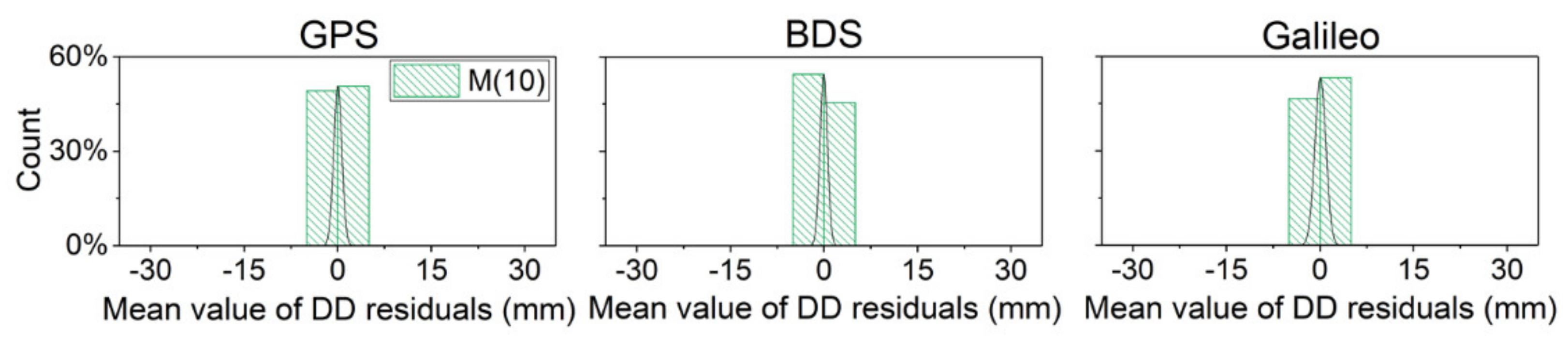
The following statistics were also gathered regarding the average value of the double-differenced residuals with multipath error correction strategy M (10) in the verification days. Compared with the statistical results in
Figure 5 and
Figure 7, the data distribution with error correction strategy M (10) was more concentrated than M (1) in
Figure 5.
In this section, the one-hour static positioning results of the verification day with error correction strategy M (10) were also counted to show the influence of the model correction on the positioning results. Compared with the uncorrected solutions in the strong multipath environment, the 3D positioning accuracy of Station A with M (10) correction increased by 84.1%, and that of station B in a normal environment reached 63.5%, which were both better than those of M (1). Therefore, the modeling of multi-day could further improve the accuracy of MHGMs and avoid the phenomenon where the lack of modeling observations in M (1) led to a poor effect of multipath error correction.
4. Discussions
Derived from the formation mechanism of the multipath error, MHGM is established using the residuals of the ambiguity-fixed double-differenced carrier phase observations. The performance of this new method is compared with that of the widely used SF method, and the multi-GNSS test results show that the average improvements of double-differenced residuals after multipath error corrections with SF and MHGM are 49.6% and 53.7%, respectively. The further power spectrum analysis of the double-differenced residuals and the static positioning results demonstrate that the performances of MHGM and SF are also comparable. This implies that the space domain MHGM can obtain similar correction effects as the SF method in the observation domain.
On the other hand, considering the characteristics of multipath error modeling in the space domain, the effectiveness of MHGM will be slightly better than that of the SF method in the observation domain. As various data on different time spans and from different satellites can be utilized together to obtain the multipath error in a certain direction of the station, the established MHGM will be much more accurate. Furthermore, with the help of the hemispherical grid in the MHGM, the distribution of the multipath error around the station in any directions can be described. On the contrary, the multipath correction models in the observation domain will be limited to certain directions by their selected satellites, and the accuracy of the corresponding model is also limited.
Furthermore, the performance of the SF method in the observation domain relies heavily on the actual orbit repeat periods of the different GNSS satellites [
22], but their orbit repeat periods are in fact different, even in the same system or constellation. For the double-differenced observation residuals, this will inevitably introduce certain errors and has a negative impact on the multipath error modeling in the observation domain. Similarly, if observations with a relative low sampling rate are used, the effectiveness of the SF method will be significantly reduced [
8], but this is not an issue for the MHGM method in the space domain.
We also found that the established MHGM using data with multi orbit repeat periods outperforms that with only one orbital repeat period, and an average improvement of 13.1% in the RMS of the double-differenced residuals is achieved. This demonstrates that the utilization of multi-day data for modeling can further improve the effectiveness of the MHGM.
5. Conclusions
In order to realize the application of the SF method in multi-GNSS multipath elimination, in this research, we analyzed the time shifts of orbit repeat periods for different systems from different days in 2018 and 2020. The time shifts of orbit repeat period for satellites in the same types of constellation are relatively stable in the long-term statistical results. The orbit repeat periods of the satellites in BDS2 are consistent with those of satellites in the same type of constellation in BDS3. After numerical investigations, we found that in the BDS system, the time shifts in (2) can be set as 246s, 246s, and 1700s for GEO, IGSO, and MEO satellites, respectively, and the time shift of the Galileo satellites can be set to a mean value of 2424s. Through the above statistical results, we have successfully expanded the SF method to both BDS3 and Galileo systems, and realized the multi-GNSS multipath error mitigation in the observation domain.
Furthermore, considering the inconvenience of utilizing the SF method for multi-GNSS multipath error modeling, we present a space domain multipath error mitigation method called MHGM. The space domain MHGM demonstrates similar correction effects as the SF method in the observation domain, but the former is more flexible for multipath error modeling in multi-GNSS data processing. Moreover, modeling the multipath error using multi-day data can further improve the effectiveness of the MHGM to a certain degree.


 ,
, 


