
Advancing Tassel Detection and Counting: Annotation and Algorithms


Abstract
:
1. Introduction
- (1)
- Regression-based techniques: These methods can only count, as they regress the local count calculated from the density map, usually estimating non-integer counts. More information about the tassel’s location and number—for example, the number of true positives (TP), false positives (FP), and false negatives (FN)—cannot be determined. However, these techniques are faster than detection-based approaches. TasselNetv2+, which was introduced to count tassels based on regression CNN [17], has undergone multiple improvements through subsequent implementations. Visual context was added to the local patches in the CNN in TasselNetv2 [18], and the first layer of the CNN was modified with global average pooling and implemented using PyTorch in TasselNetv2+ [19]. All three implementations use point annotation.
- (2)
- Detection-based techniques: These approaches are categorized as anchor-based and anchor-free. Anchor-based approaches include one- and two-stage detectors and are based on bounding box annotation. Single-stage detectors consider object detection as a dense classification and localization problem [20,21,22,23]. They are faster and simpler, but detection accuracy is usually lower than two- or multi-stage detectors. Two-stage detectors first generate the object proposals, and then, in the second stage, the features are extracted from the candidate proposals [24,25,26,27]. These detectors have high localization and object detection accuracy. Anchor-based approaches that have been used for maize tassel detection include Faster R-CNN [24,28], Yolov3 [29], RetinaNet [4,20], and FaceBoxes [30]. Of these, Faster R-CNN obtained the highest accuracy [16,28,31]. Anchor-free detectors do not generate the anchors; therefore, the computational complexity is typically decreased. These approaches are mainly anchor-point methods (e.g., Grid R-CNN [32] and FoveaBox [33]) and key-point detectors (e.g., CornerNet [34], ExtremeNet [35], and CenterNet [36]). These techniques, which have been successfully demonstrated for other applications with similar complexity, could potentially yield higher accuracy tassel detection and counting than previously published approaches without the excessive computational overhead. To the best of our knowledge, these approaches have not been investigated for this application.
2. Materials and Methods
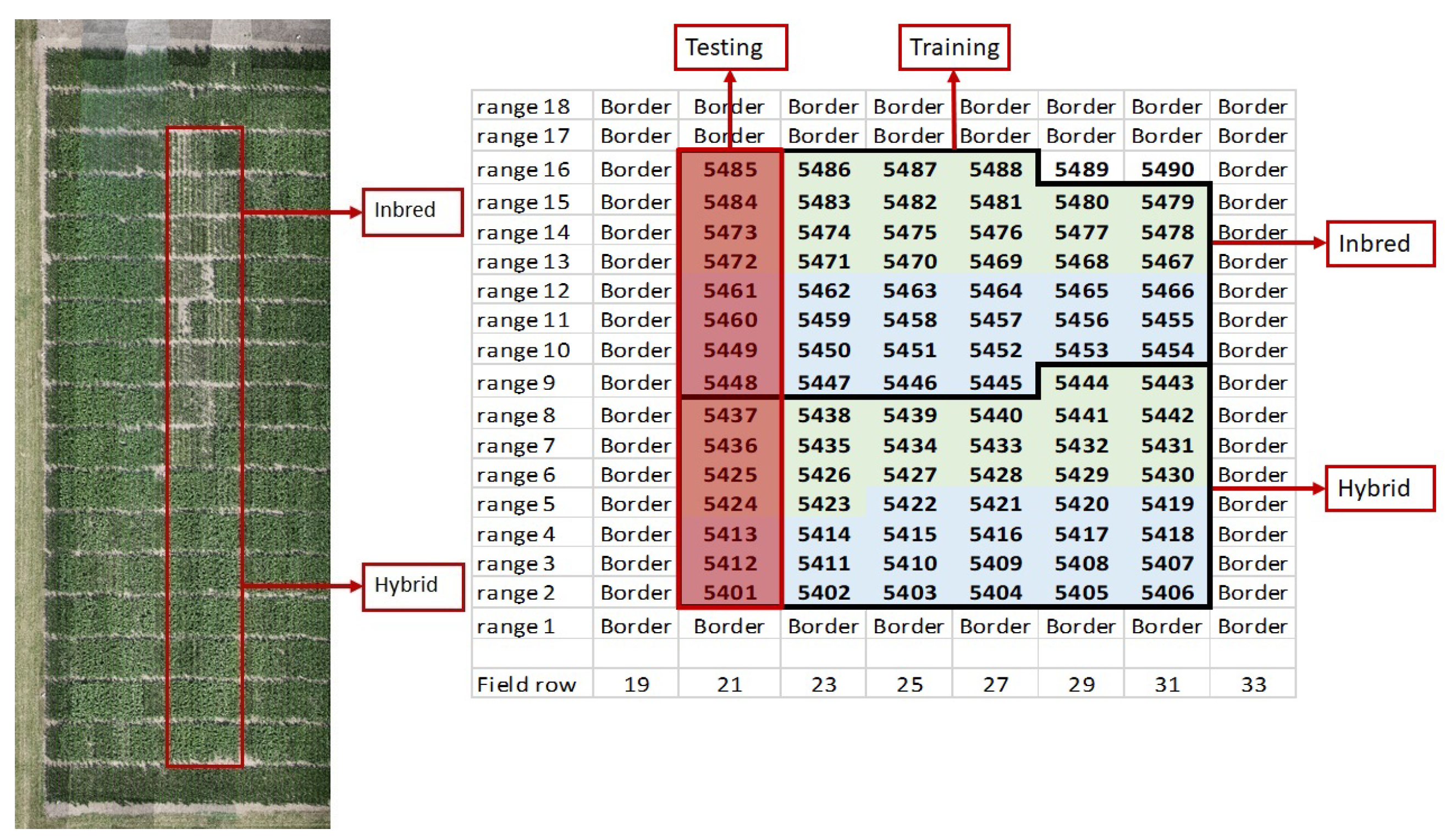
2.1. Field Experiment and Image Acquisition
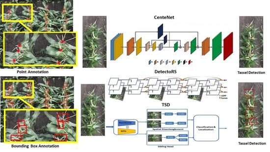
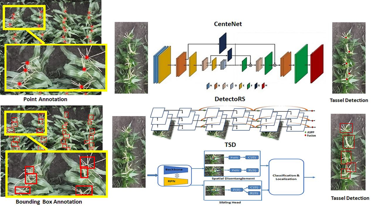
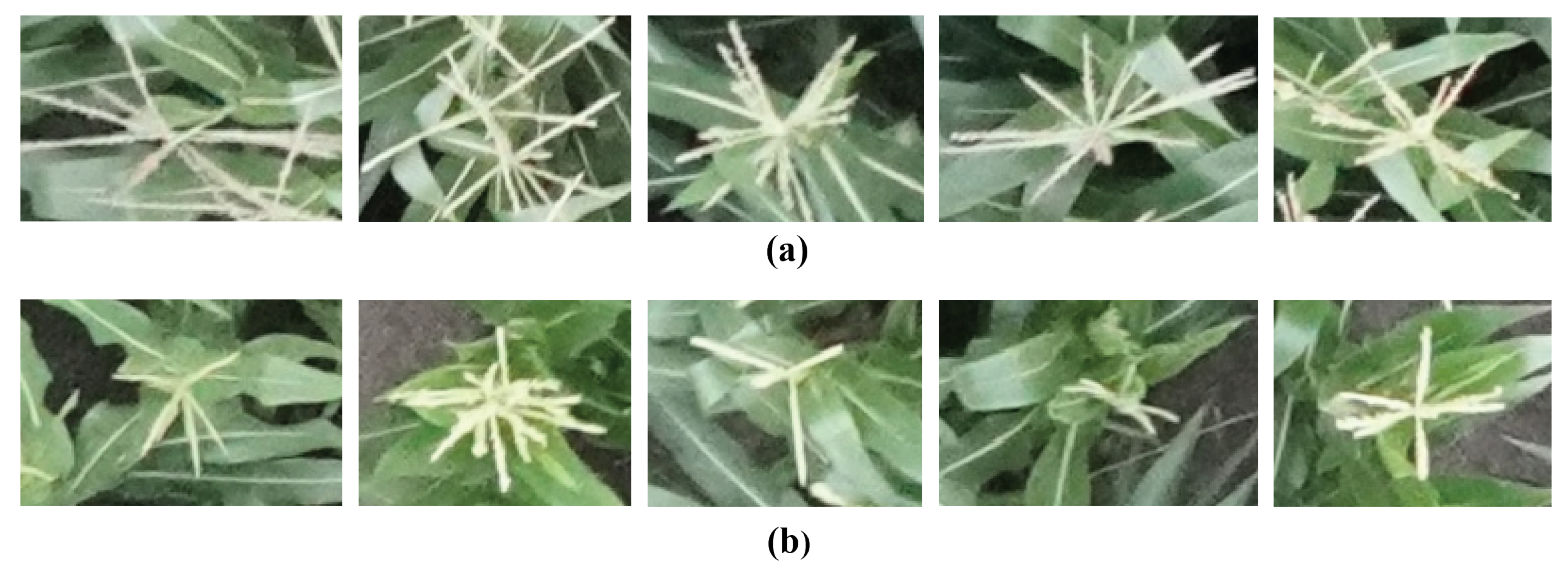
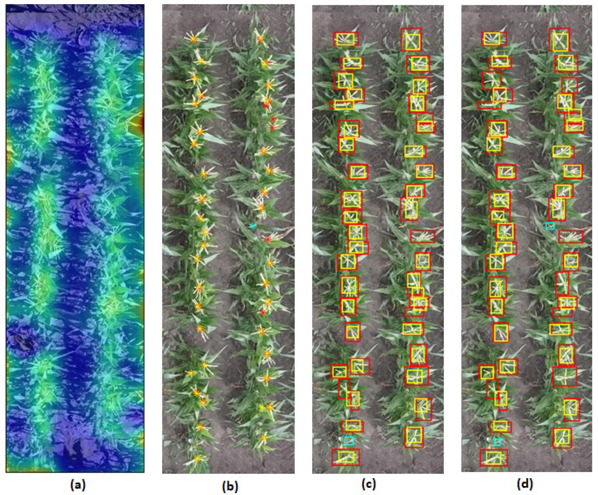
2.2. Data Annotation
2.3. Model Description
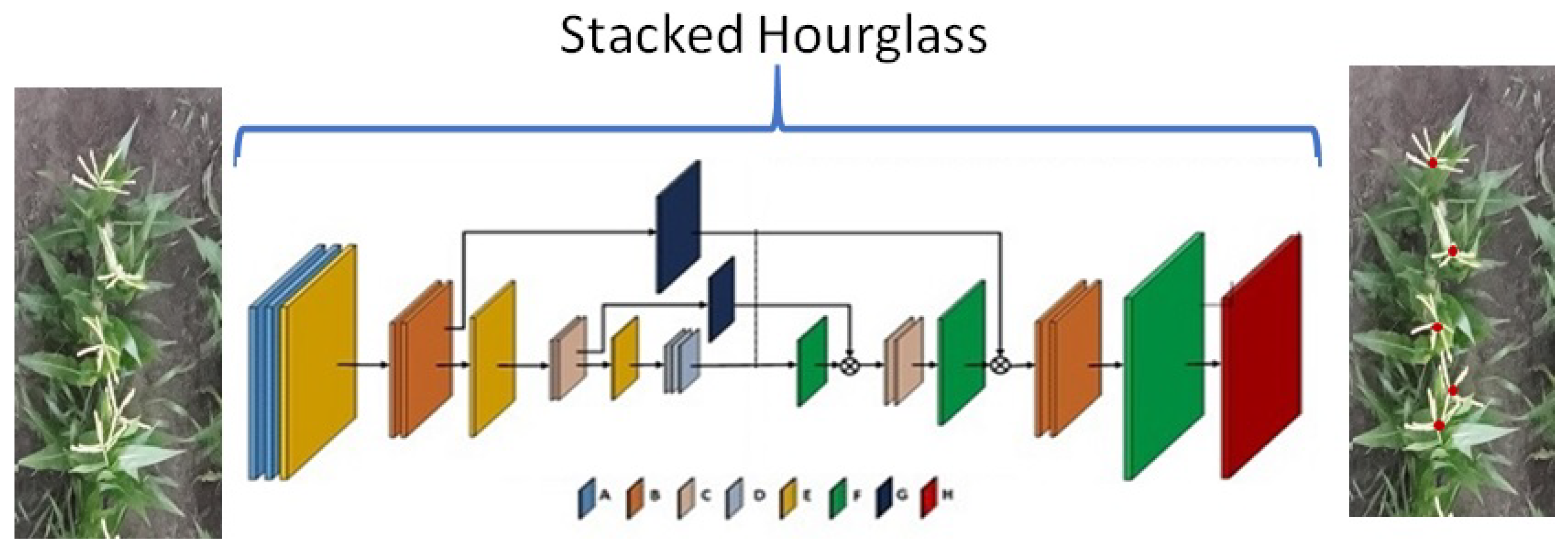
2.3.1. CenterNet
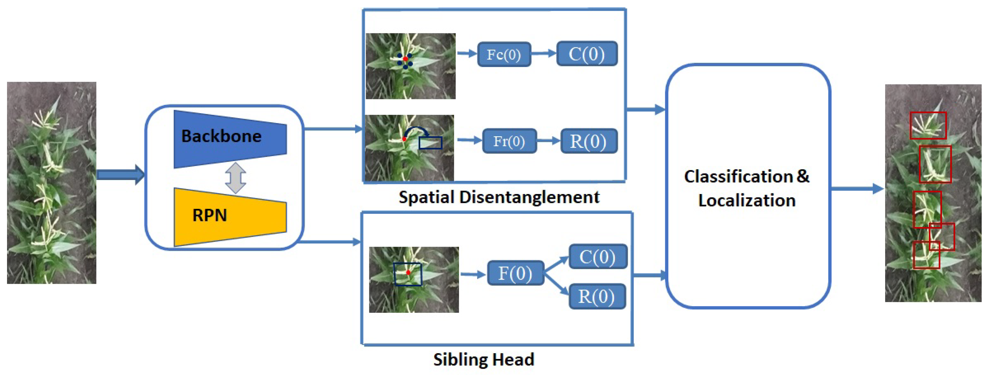
2.3.2. TSD
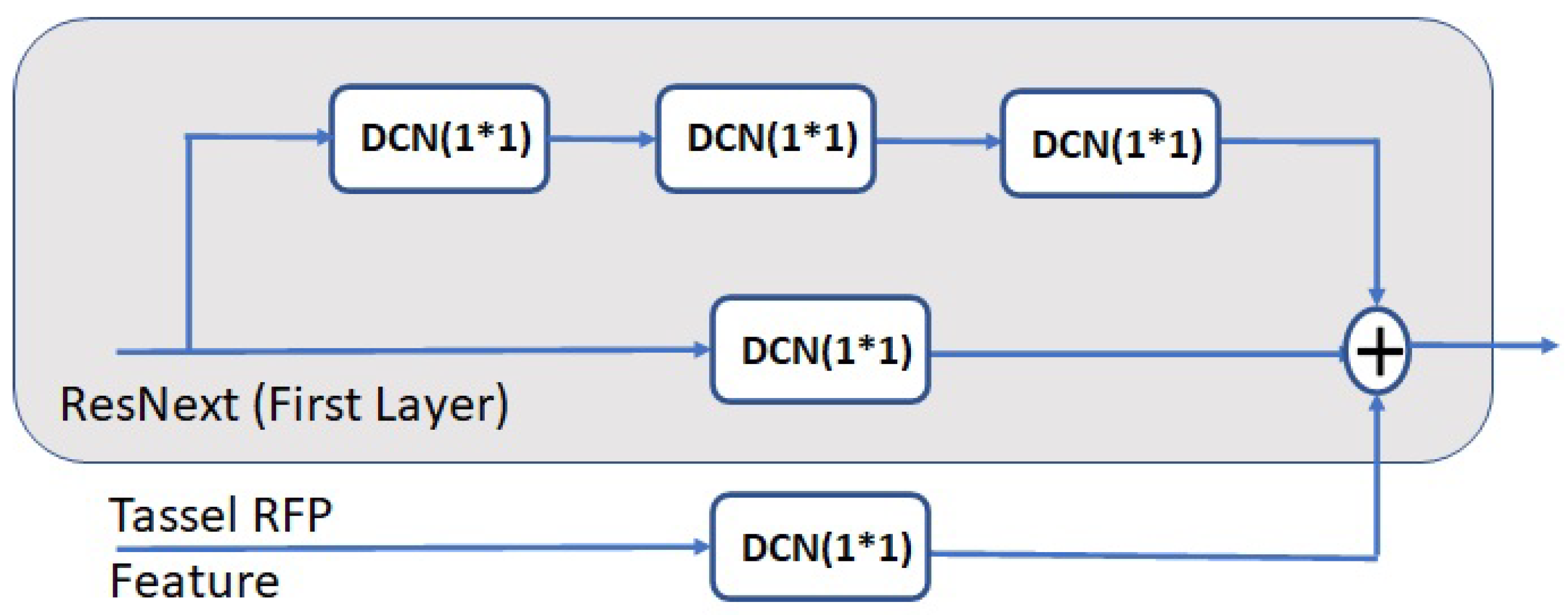
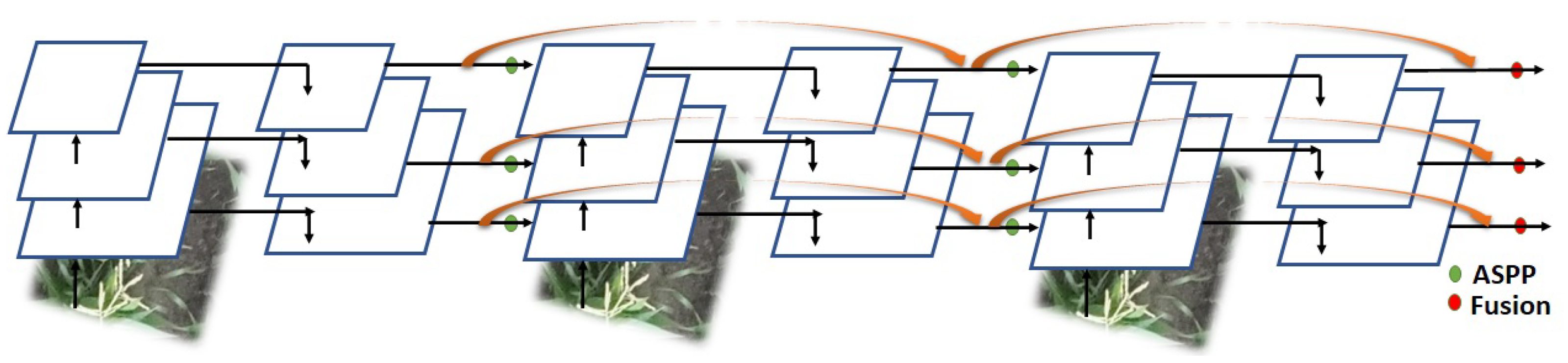
2.3.3. DetectoRS
2.3.4. TasselNetv2+
2.4. Parameter Settings
2.5. Model Evaluation
2.5.1. Detection Metrics
2.5.2. Counting Metrics
3. Results
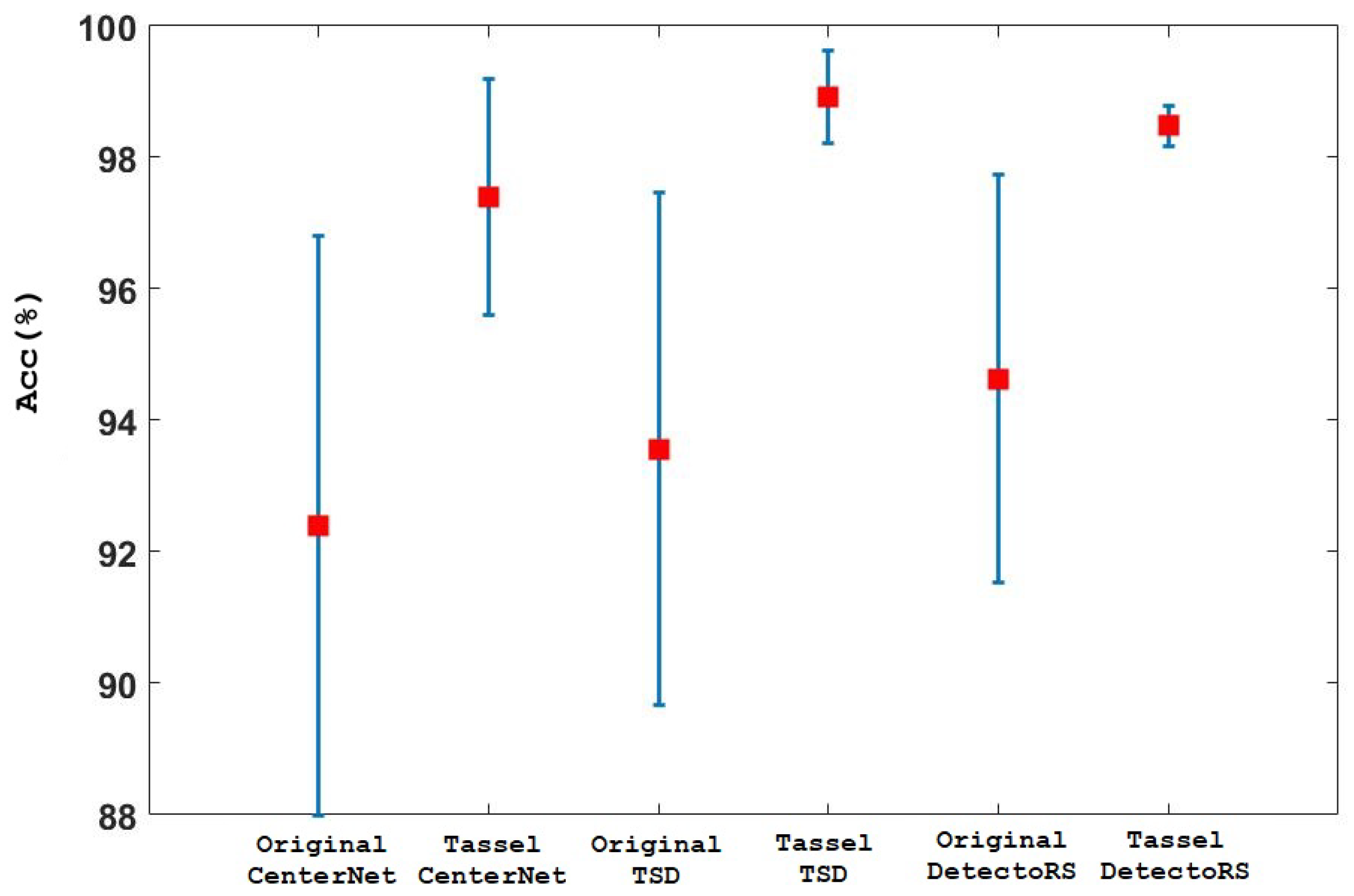
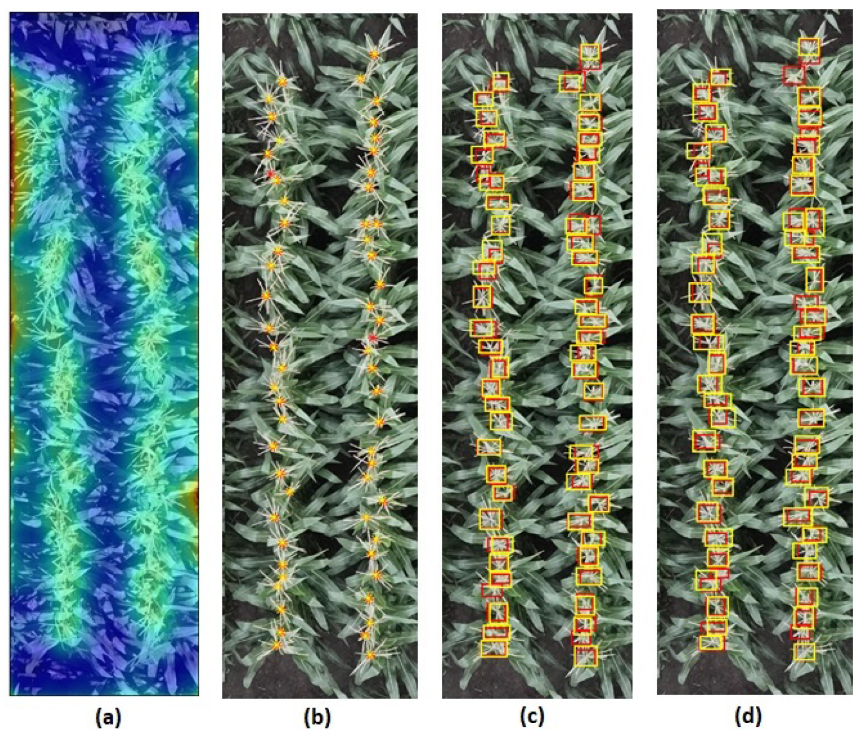
3.1. Comparison of Original and Developed Anchor and Anchor-Free Based Approaches for Tassel Detection
3.2. Sensitivity Analysis to Bounding Box Sizes
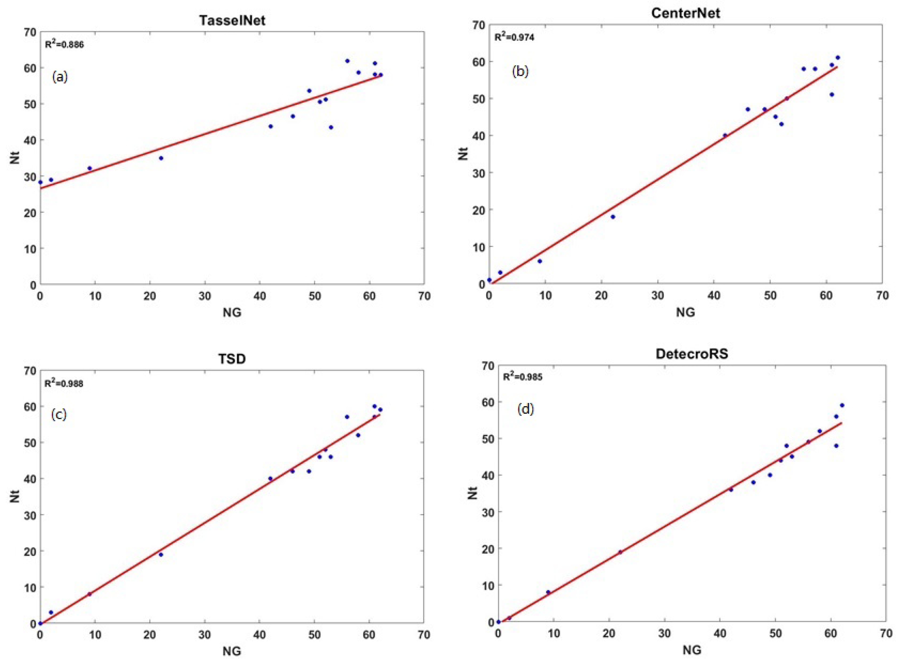
3.3. Sensitivity to Tassel Density and Heterogeneity
3.4. Training and Testing Information
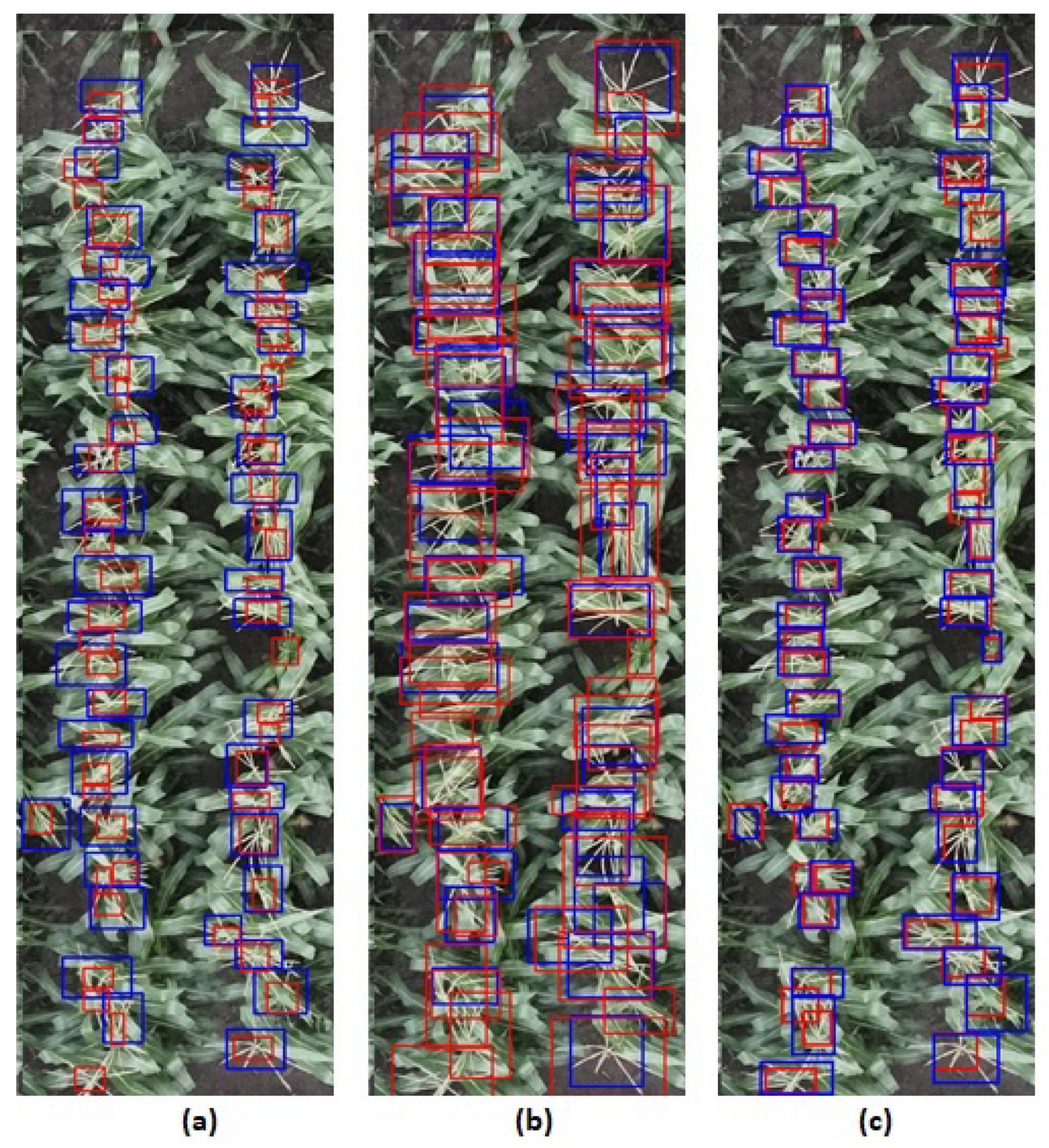
3.5. Comparison for Different Annotation Techniques
4. Conclusions
Author Contributions
Funding
Institutional Review Board Statement
Informed Consent Statement
Data Availability Statement
Acknowledgments
Conflicts of Interest
References
- Ji, M.; Yang, Y.; Zheng, Y.; Zhu, Q.; Huang, M.; Guo, Y. In-field automatic detection of maize tassels using computer vision. Inf. Process. Agric. 2021, 8, 87–95. [Google Scholar] [CrossRef]
- Su, Y.; Wu, F.; Ao, Z.; Jin, S.; Qin, F.; Liu, B.; Pang, S.; Liu, L.; Guo, Q. Evaluating maize phenotype dynamics under drought stress using terrestrial LiDAR. Plant Methods 2019, 15, 1–16. [Google Scholar] [CrossRef] [Green Version]
- Guo, W.; Fukatsu, T.; Ninomiya, S. Automated characterization of flowering dynamics in rice using field-acquired time-series RGB images. Plant Methods 2015, 11, 7. [Google Scholar] [CrossRef] [Green Version]
- Mirnezami, S.V.; Srinivasan, S.; Zhou, Y.; Schnable, P.S.; Ganapathysubramanian, B. Detection of the progression of anthesis in field-grown maize tassels: A case study. Plant Phenomics 2021, 2021, 4238701. [Google Scholar] [CrossRef]
- Karami, A.; Crawford, M.; Delp, E.J. Automatic plant counting and location based on a few-shot learning technique. IEEE J. Sel. Top. Appl. Earth Obs. Remote Sens. 2020, 13, 5872–5886. [Google Scholar] [CrossRef]
- Tian, H.; Wang, T.; Liu, Y.; Qiao, X.; Li, Y. Computer vision technology in agricultural automation—A review. Inf. Process. Agric. 2020, 7, 1–19. [Google Scholar] [CrossRef]
- Gage, J.L.; Miller, N.D.; Spalding, E.P.; Kaeppler, S.M.; de Leon, N. TIPS: A system for automated image-based phenotyping of maize tassels. Plant Methods 2017, 13, 1–12. [Google Scholar] [CrossRef] [PubMed] [Green Version]
- Ye, M.; Cao, Z.; Yu, Z. An image-based approach for automatic detecting tasseling stage of maize using spatio-temporal saliency. In Remote Sensing Image Processing, Geographic Information Systems, International Society for Optics and Photonics; SPIE: Washington, DC, USA, 2013; Volume 8921, p. 89210Z. [Google Scholar]
- Kurtulmuş, F.; Kavdir, I. Detecting corn tassels using computer vision and support vector machines. Expert Syst. Appl. 2014, 41, 7390–7397. [Google Scholar] [CrossRef]
- Osco, L.P.; Junior, J.M.; Ramos, A.P.M.; Jorge, L.A.C.; Fatholahi, S.N.; Silva, J.A.; Matsubara, E.T.; Gonçalves, W.N.; Pistori, H.; Li, J. A review on deep learning in UAV remote sensing. arXiv 2021, arXiv:2101.10861. [Google Scholar]
- Karami, A.; Crawford, M.; Delp, E.J. A weakly supervised deep learning approach for plant center detection and counting. In Proceedings of the IGARSS 2020—2020 IEEE International Geoscience and Remote Sensing Symposium, Waikoloa, HI, USA, 26 September–2 October 2020; pp. 1584–1587. [Google Scholar]
- Valente, J.; Sari, B.; Kooistra, L.; Kramer, H.; Mücher, S. Automated crop plant counting from very high-resolution aerial imagery. Precis. Agric. 2020, 21, 1366–1384. [Google Scholar] [CrossRef]
- Hasan, M.M.; Chopin, J.P.; Laga, H.; Miklavcic, S.J. Detection and analysis of wheat spikes using convolutional neural networks. Plant Methods 2018, 14, 1–13. [Google Scholar] [CrossRef] [Green Version]
- Ghosal, S.; Zheng, B.; Chapman, S.C.; Potgieter, A.B.; Jordan, D.R.; Wang, X.; Singh, A.K.; Singh, A.; Hirafuji, M.; Ninomiya, S.; et al. A weakly supervised deep learning framework for sorghum head detection and counting. Plant Phenomics 2019, 2019, 1525874. [Google Scholar] [CrossRef] [Green Version]
- Yang, K.; Zhong, W.; Li, F. Leaf segmentation and classification with a complicated background using deep learning. Agronomy 2020, 10, 1721. [Google Scholar] [CrossRef]
- Zou, H.; Lu, H.; Li, Y.; Liu, L.; Cao, Z. Maize tassels detection: A benchmark of the state of the art. Plant Methods 2020, 16, 108. [Google Scholar] [CrossRef]
- Lu, H.; Cao, Z.; Xiao, Y.; Zhuang, B.; Shen, C. TasselNet: Counting maize tassels in the wild via local counts regression network. Plant Methods 2017, 13, 79. [Google Scholar] [CrossRef] [PubMed] [Green Version]
- Xiong, H.; Cao, Z.; Lu, H.; Madec, S.; Liu, L.; Shen, C. TasselNetv2: In-field counting of wheat spikes with context-augmented local regression networks. Plant Methods 2019, 15, 150. [Google Scholar] [CrossRef] [PubMed]
- Lu, H.; Cao, Z. TasselNetV2+: A fast implementation for high-throughput plant counting from high-resolution RGB imagery. Front. Plant Sci. 2020, 11, 1929. [Google Scholar] [CrossRef]
- Lin, T.Y.; Goyal, P.; Girshick, R.; He, K.; Dollár, P. Focal loss for dense object detection. In Proceedings of the 2017 IEEE Conference on Computer Vision and Pattern Recognition (CVPR), Honolulu, HI, USA, 21–26 July 2017; pp. 2980–2988. [Google Scholar]
- Li, X.; Wang, W.; Wu, L.; Chen, S.; Hu, X.; Li, J.; Tang, J.; Yang, J. Generalized focal loss: Learning qualified and distributed bounding boxes for dense object detection. In Proceedings of the 2020 Conference on Neural Information Processing Systems, NeurIPS, Vancouver, BC, Canada, 21–22 December 2020. [Google Scholar]
- Li, X.; Wang, W.; Hu, X.; Li, J.; Tang, J.; Yang, J. Generalized focal loss V2: Learning reliable localization quality estimation for dense object detection. arXiv 2020, arXiv:2011.12885. [Google Scholar]
- Shinya, Y. USB: Universal-scale object detection benchmark. arXiv 2021, arXiv:2103.14027. [Google Scholar]
- Ren, S.; He, K.; Girshick, R.; Sun, J. Faster R-CNN: Towards real-time object detection with region proposal networks. IEEE Trans. Pattern Anal. Mach. Intell. 2016, 39, 1137–1149. [Google Scholar] [CrossRef] [Green Version]
- Song, G.; Liu, Y.; Wang, X. Revisiting the sibling had in object detector. In Proceedings of the IEEE Conference on Computer Vision and Pattern Recognition, Seattle, WA, USA, 14–19 June 2020; pp. 11560–11569. [Google Scholar] [CrossRef]
- Sun, Z.; Cao, S.; Yang, Y.; Kitani, K. Rethinking transformer-based set prediction for object detection. arXiv 2020, arXiv:2011.10881. [Google Scholar]
- Qiao, S.; Chen, L.C.; Yuille, A. DetectoRS: Detecting objects with recursive feature pyramid and switchable atrous convolution. arXiv 2020, arXiv:2006.02334. [Google Scholar]
- Liu, Y.; Cen, C.; Che, Y.; Ke, R.; Ma, Y.; Ma, Y. Detection of maize tassels from UAV RGB imagery with faster R-CNN. Remote Sens. 2020, 12, 338. [Google Scholar] [CrossRef] [Green Version]
- Redmon, J.; Farhadi, A. Yolov3: An incremental improvement. arXiv 2018, arXiv:1804.02767. [Google Scholar]
- Zhang, S.; Zhu, X.; Lei, Z.; Shi, H.; Wang, X.; Li, S.Z. Faceboxes: A CPU real-time face detector with high accuracy. In Proceedings of the International Joint Conference on Biometrics, Denver, CO, USA, 1–4 October 2017; pp. 1–9. [Google Scholar]
- Kumar, A.; Taparia, M.; Rajalakshmi, P.; Desai, U.; Naik, B.; Guo, W. UAV based remote sensing for tassel detection and growth stage estimation of maize crop using F-RCNN. Comput. Vis. Probl. Plant Phenotyping 2019, 3, 4321–4323. [Google Scholar]
- Lu, X.; Li, B.; Yue, Y.; Li, Q.; Yan, J. Grid R-CNN. In Proceedings of the IEEE Conference on Computer Vision and Pattern Recognition, Long Beach, CA, USA, 16–20 June 2019; pp. 7363–7372. [Google Scholar]
- Kong, T.; Sun, F.; Liu, H.; Jiang, Y.; Li, L.; Shi, J. Foveabox: Beyound anchor-based object detection. IEEE Trans. Image Process. 2020, 29, 7389–7398. [Google Scholar] [CrossRef]
- Law, H.; Deng, J. Cornernet: Detecting objects as paired keypoints. In Proceedings of the European Conference on Computer Vision, Munich, Germany, 8–14 September 2018; pp. 734–750. [Google Scholar]
- Zhou, X.; Zhuo, J.; Krahenbuhl, P. Bottom-up object detection by grouping extreme and center points. In Proceedings of the IEEE Conference on Computer Vision and Pattern Recognition, Long Beach, CA, USA, 16–20 June 2019; pp. 850–859. [Google Scholar]
- Zhou, X.; Wang, D.; Krähenbühl, P. Objects as points. arXiv 2019, arXiv:1904.07850. [Google Scholar]
- Lin, Y.C.; Zhou, T.; Wang, T.; Crawford, M.; Habib, A. New orthophoto generation strategies from UAV and ground remote sensing platforms for high-throughput phenotyping. Remote Sens. 2021, 13, 860. [Google Scholar] [CrossRef]
- The Genomes to Fields Initiative (G2F). Standard Operating Procedures (SOP). 2020. Available online: https://www.genomes2fields.org/resources/ (accessed on 22 April 2021).
- Wada, K. Labelme: Image Polygonal Annotation with Python. 2018. Available online: https://github.com/wkentaro/labelme (accessed on 9 May 2016).
- Cai, Z.; Vasconcelos, N. Cascade R-CNN: High quality object detection and instance segmentation. arXiv 2019, arXiv:1906.09756. [Google Scholar] [CrossRef] [Green Version]
- Dai, J.; Qi, H.; Xiong, Y.; Li, Y.; Zhang, G.; Hu, H.; Wei, Y. Deformable convolutional networks. In Proceedings of the 2017 IEEE Conference on Computer Vision and Pattern Recognition, Honolulu, HI, USA, 21–26 July 2017; pp. 764–773. [Google Scholar]
- Chen, L.C.; Papandreou, G.; Kokkinos, I.; Murphy, K.; Yuille, A.L. Semantic image segmentation with deep convolutional nets and fully connected CRFS. arXiv 2014, arXiv:1412.7062. [Google Scholar]
- Papandreou, G.; Kokkinos, I.; Savalle, P.A. Modeling local and global deformations in deep learning: Epitomic convolution, multiple instance learning, and sliding window detection. In Proceedings of the 2015 IEEE Conference on Computer Vision and Pattern Recognition, Boston, MA, USA, 7–12 June 2015; pp. 390–399. [Google Scholar]
- Hu, J.; Shen, L.; Sun, G. Squeeze-and-excitation networks. In Proceedings of the 2018 IEEE Conference on Computer Vision and Pattern Recognition, Salt Lake City, UT, USA, 18–22 June 2018; pp. 7132–7141. [Google Scholar]


| Parameter | CenterNet | TSD | DetectoRS | TasselNetv2+ |
|---|---|---|---|---|
| Model | ExtremeNet | CascadeRCNN | CascadeRCNN | - |
| Backbone | Hourglass | ResNeXt+DCN | ResNeXt | - |
| Depth | 104 | 101 | 101 | - |
| Batch Size | 11 | 2 | 2 | 16 |
| Epochs | 240 | 500 | 500 | 300 |
| Optimizer | Adam | SGD | SGD | SGD |
| Learning Rate (lr) | 1.25 | 1.25 | 1.25 | 1.25 |
| Gaussian Kernel Parameter | - | - | - | 6 |
| Technique | Image Size | No. Training | No. Validation | No. Test | Training Time |
|---|---|---|---|---|---|
| TasselNetv2+ | 2100 × 600 | 97 | 8 | 15 | 1 h & 23 min |
| CenterNet | 512 × 512 | 350 | 30 | 15 | 7 h & 34 min |
| TSD | 2100 × 600 | 97 | 8 | 15 | 8 h & 41 min |
| DetectoRS | 2100 × 600 | 97 | 8 | 15 | 7 h & 57 min |
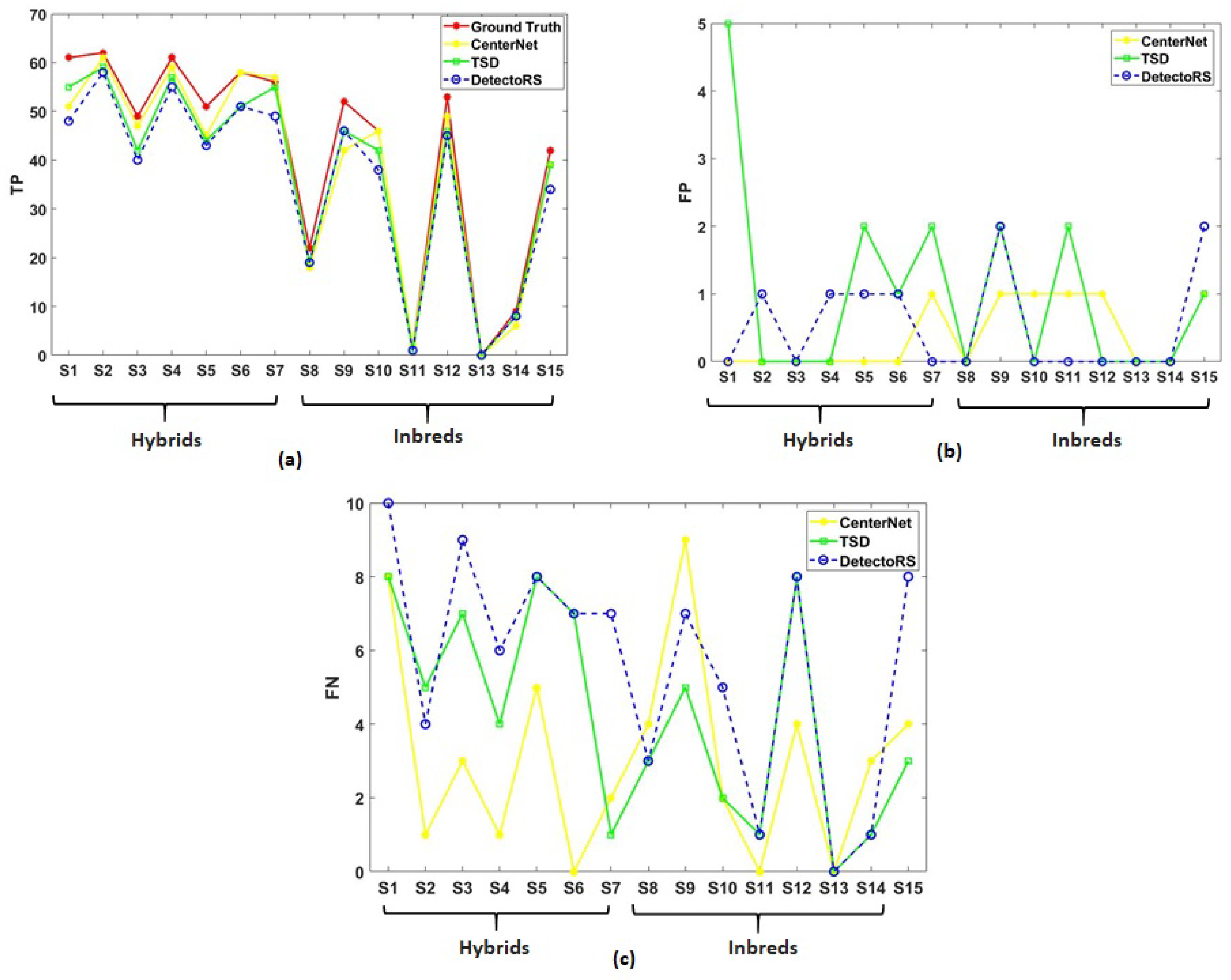
| Technique | Metric | TP | FP | FN | Nt | Ng | Pr | Re | SC |
|---|---|---|---|---|---|---|---|---|---|
| CenterNet | Mean | 38.67 | 0.40 | 3.07 | 39.13 | 41.93 | 96.86 | 90.97 | 93.24 |
| Std Dev | 21.36 | 0.51 | 2.74 | 21.25 | 22.17 | 8.75 | 9.24 | 6.46 | |
| TSD | Mean | 37.60 | 1.00 | 4.20 | 38.60 | 41.60 | 93.47 | 87.02 | 89.90 |
| Std Dev | 20.38 | 1.41 | 2.88 | 20.76 | 22.86 | 17.49 | 11.42 | 14.59 | |
| DetectoRS | Mean | 35.67 | 0.53 | 5.60 | 36.20 | 41.60 | 98.76 | 83.86 | 90.30 |
| Std Dev | 19.33 | 0.74 | 3.14 | 19.64 | 22.03 | 1.79 | 10.33 | 7.15 |
| Method | MAE | RMSE |
|---|---|---|
| TasselNetv2+ | 8.628 | 77.88 |
| CenterNet | 3.333 | 12.91 |
| TSD | 3.270 | 13.43 |
| DetectoRS | 5.400 | 20.94 |
| Testing Plot | Flowering Date | Ng | CenterNet | TSD | DetectoRS |
|---|---|---|---|---|---|
| S1 | 13-July | 61 | 92.72 | 89.43 | 90.56 |
| S2 | 13-July | 62 | 99.18 | 95.93 | 95.86 |
| S3 | 17-July | 49 | 96.90 | 92.30 | 89.88 |
| S4 | 18-July | 61 | 99.15 | 96.60 | 94.01 |
| S5 | 20-July | 51 | 94.73 | 89.79 | 90.52 |
| S6 | 17-July | 58 | 100.00 | 91.84 | 92.72 |
| S7 | 15-July | 56 | 97.43 | 97.34 | 93.33 |
| S8 | 22-July | 22 | 89.99 | 92.68 | 93.76 |
| S9 | 9-July | 52 | 89.35 | 92.92 | 91.08 |
| S10 | 22-July | 46 | 96.83 | 97.67 | 93.82 |
| S11 | 16-July | 2 | 80.00 | 39.99 | 66.66 |
| S12 | 26-July | 53 | 95.14 | 91.99 | 91.83 |
| S13 | 20-July | 0 | - | - | - |
| S14 | 25-July | 9 | 79.99 | 94.11 | 95.37 |
| S15 | 22-July | 42 | 93.97 | 95.11 | 87.17 |
Publisher’s Note: MDPI stays neutral with regard to jurisdictional claims in published maps and institutional affiliations. |
© 2021 by the authors. Licensee MDPI, Basel, Switzerland. This article is an open access article distributed under the terms and conditions of the Creative Commons Attribution (CC BY) license (https://creativecommons.org/licenses/by/4.0/).
Share and Cite
Karami, A.; Quijano, K.; Crawford, M. Advancing Tassel Detection and Counting: Annotation and Algorithms. Remote Sens. 2021, 13, 2881. https://doi.org/10.3390/rs13152881
Karami A, Quijano K, Crawford M. Advancing Tassel Detection and Counting: Annotation and Algorithms. Remote Sensing. 2021; 13(15):2881. https://doi.org/10.3390/rs13152881
Chicago/Turabian StyleKarami, Azam, Karoll Quijano, and Melba Crawford. 2021. "Advancing Tassel Detection and Counting: Annotation and Algorithms" Remote Sensing 13, no. 15: 2881. https://doi.org/10.3390/rs13152881
APA StyleKarami, A., Quijano, K., & Crawford, M. (2021). Advancing Tassel Detection and Counting: Annotation and Algorithms. Remote Sensing, 13(15), 2881. https://doi.org/10.3390/rs13152881