Abstract
Although ionosphere-free (IF) combination is usually employed in long-range precise positioning, in order to employ the knowledge of the spatiotemporal ionospheric delays variations and avoid the difficulty in choosing the IF combinations in case of triple-frequency data processing, using uncombined observations with proper ionospheric constraints is more beneficial. Yet, determining the appropriate power spectral density (PSD) of ionospheric delays is one of the most important issues in the uncombined processing, as the empirical methods cannot consider the actual ionosphere activities. The ionospheric delays derived from actual dual-frequency phase observations contain not only the real-time ionospheric delays variations, but also the observation noise which could be much larger than ionospheric delays changes over a very short time interval, so that the statistics of the ionospheric delays cannot be retrieved properly. Fortunately, the ionospheric delays variations and the observation noise behave in different ways, i.e., can be represented by random-walk and white noise process, respectively, so that they can be separated statistically. In this paper, we proposed an approach to determine the PSD of ionospheric delays for each satellite in real-time by denoising the ionospheric delay observations. Based on the relationship between the PSD, observation noise and the ionospheric observations, several aspects impacting the PSD calculation are investigated numerically and the optimal values are suggested. The proposed approach with the suggested optimal parameters is applied to the processing of three long-range baselines of 103 km, 175 km and 200 km with triple-frequency BDS data in both static and kinematic mode. The improvement in the first ambiguity fixing time (FAFT), the positioning accuracy and the estimated ionospheric delays are analysed and compared with that using empirical PSD. The results show that the FAFT can be shortened by at least 8% compared with using a unique empirical PSD for all satellites although it is even fine-tuned according to the actual observations and improved by 34% compared with that using PSD derived from ionospheric delay observations without denoising. Finally, the positioning performance of BDS three-frequency observations shows that the averaged FAFT is 226 s and 270 s, and the positioning accuracies after ambiguity fixing are 1 cm, 1 cm and 3 cm in the East, North and Up directions for static and 3 cm, 3 cm and 6 cm for kinematic mode, respectively.
1. Introduction
For medium- and long-range relative positioning in both static and Real-Time Kinematic (RTK) mode, one of the most significant impact factors is the ionospheric delays, which are increasing with the inter-station distance [1]. There are two major methods dealing with ionospheric delays: on the one hand, it can be eliminated based on its frequency dependency by forming ionosphere-free (IF) observations using dual-frequency observations, which is still the most common and effective method until now [2]. On the other hand, the slant ionospheric delays are estimated as unknown epoch-wise using uncombined observations [3,4]. In principle, the IF observation is derived from the latter one by eliminating ionosphere delays parameters at the observation level. However, using IF observations has the following three disadvantages.
In the combination, taking dual-frequency data as an example, for a station-satellite pair, there are four observations, two for each phase and range, after eliminating the ionospheric parameter, only two IF observations are formed for phase and range, respectively. Obviously, this combination is rank-defected and cannot retain all observation information. The reason is that while forming IF observations, the ionospheric slant delays parameter in phase and range observations is eliminated as different ones. One consequence is that the noise of the IF observations is enlarged according to the law of error propagation and the estimates will be degraded accordingly. Theoretically, if the full covariance matrix is considered, using original observations or their full-rank linear combination gives the same solution [5].
From the study of the ionosphere, the ionosphere variation has good statistical characteristics in space and time, which can be obtained from establishing an a priori model to efficiently constrain ionospheric parameters to enhance the solution. In the case of using IF observations, it is impossible to impose such statistical constraints as the ionosphere delays parameters are already eliminated.
Last but not least, more and more Global Navigation Satellite Systems (GNSS) provide multi-frequency signals, for example, the Chinese BeiDou Navigation Satellite System (BDS) which is the first GNSS providing triple-frequency signals across the whole constellation [6]. The triple-frequency data is obviously conducive to increasing the redundancy of parameter estimation. More importantly, it can significantly improve the efficiency and reliability of the carrier phase integer ambiguity resolution which is essential for precise positioning [7,8]. IF observations are used, we have to decide which IF observations should be used in the processing.
In comparison with using IF observations, the latter one takes the observations of all frequencies and is modelled in a unified and simple way, and the slant ionospheric delays of all observations of a station-satellite pair are modelled according to the relations among pseudo-range and phase, and signal frequencies, and only one slant ionospheric delays are estimated as unknown parameters. In this case, it is convenient to introduce the prior information into the parameter estimation in the form of constraints. Therefore, it can be seen that using uncombined observations is more conducive to the data processing of multi-system and multi-frequency fusion. This is also one of the reasons why the undifferenced and uncombined observation model is becoming a research hotspot [9,10].
The ionospheric delays depend on the total electron content (TEC) along the signal propagation path, which is a function of a number of variables, including solar ionization flux, magnetic field activity [11]. Its temporal and spatial correlation is easy to understand from GNSS observations. For example, the ionospheric delays of two nearby stations to the same satellite should be the same and their difference gets larger along with the inter-station distance. Similarly, the difference between the two adjacent epochs is rather small. Therefore, a number of studies were carried out to investigate the ionosphere characteristics in order to properly quantify these correlations for obtaining appropriate spatiotemporal ionospheric delays constraints [12]. Besides the temporal and spatial constraints, a priori ionospheric corrections from a reconstructed model such as the global ionospheric map or nearby reference stations in network RTK can also be considered while constructing the constraints [13,14,15,16].
In principle, the spatiotemporal variation of ionospheric delays can be represented by a random walk process with the PSD as its critical parameter which decides the strengths of the constraint [17]. The relative spatial variation between two stations depends on the inter-station distance. For short baselines the variation is negligible, i.e., the two stations have almost the same ionospheric delays and can be fully cancelled in the inter-station difference. Differently from precise point positioning, in relative positioning, the ionospheric delays can be reduced or eliminated in the inter-station difference and the residual ionospheric delays are rather small depending on the inter-station distance [18]. It is worth pointing out that in RTK the inter-station differenced ionospheric delay is estimated and its variation is rather small depending somehow on the baseline length.
Bock proposed a method of incorporating prior information on residual ionospheric effects in the form of weighted constraints in order to improve phase ambiguity resolution [19]. It was successful in unifying the processing algorithm for short and long baselines by imposing ionospheric constraints according to baseline length. This was further improved by Schafferin and Bock and was widely used later on [4]. Teunissen investigated theoretically the impact of weighted ionospheric delays considering both the spatial and temporal variation in ambiguity resolution [20]. Goad and Yang developed a two-dimension model to simultaneously consider the spatial and temporal correlation, i.e., baseline length and observations sampling interval, respectively, based on the autocorrelation of the estimated ionospheric delays [21]. Odijk proposed a priori ionospheric weight as a function of the baseline length [22]. There are also several studies on the ionospheric constraints for network RTK [23,24,25] and for precise point positioning [26,27].
In the above-mentioned methods, the PSD of the ionospheric delays parameterized as a random walk process is usually obtained empirically or based on previous data. Therefore, it cannot always accurately describe the current status, especially if there are temporal and spatial variations of small scale [28]. Liu and Lachapelle analyzed the influence of different random walk parameters on the ionospheric delays estimates and the fixation of ambiguity [29]. Schaer also demonstrated that using empirical prior variant is difficult in capturing the spatial and temporal changes of small scale [30]. Furthermore, statistics based on the estimated ionospheric delays are more suitable but cannot be implemented easily for real-time processing.
The ionospheric observations, obtained by the combination of carrier phase observations, can accurately reflect the temporal fluctuation of the ionospheric path delays, so can be used for deriving more accurate ionospheric statistics for appropriate constraints. For example, Pi proposed a rate of change of total electron content index (ROTI) [31], which can be derived from dual-frequency phase observations, to monitor ionospheric scintillation. In fact, the ionospheric observation is a superposition of phase observation noise and ionospheric delays. The observation noise is usually considered as white noise, although high sampling data is temporally correlated, while ionospheric delays are represented by a random walk process as aforesaid. Ignoring the short-term temporal correlation of the observation noise, its standard deviation (STD) is about 0.01 cycle, i.e., 2 mm and could be enlarged to 2 to 3 times due to environmental impact at low elevations. However, the ionospheric variation within a few seconds is most likely much smaller than the noise, so the change of the ionosphere between-epochs will be overwhelmed by the observation noise. Therefore, we cannot directly use the STD of the epoch-differenced ionosphere (EDI) observations to qualify the actual ionospheric variation. Fortunately, the ionospheric variation increases in the EDI observations along with the differential interval of the two epochs, while the observation noise stays unchanged. Hence, the two superposed parts can be separated due to the different attributes. Therefore, we will study characteristics of the ionospheric observations and develop a new approach to quickly estimate accurate PSD from ionospheric observations by suppressing observation noise, and apply the estimated PSD to constrain ionospheric delays parameters for real-time precise positioning.
The paper is arranged as follows: the related functional and stochastical models will be introduced focusing on the handling of ionospheric delays. Then, the temporal correlation of ionospheric delays is investigated based on the ionospheric observations. Afterwards, a new approach for PSD estimation based on the ionospheric observations is presented and several related aspects are evaluated. The efficiency of the new approach is validated by comparing it with the existing ones before conclusions are drawn.
2. Model of Long-Range RTK
2.1. Basic Observation Equations
The observation equations of inter-station difference using the BDS carrier phase observation in unit of meter, and the pseudo-range observation at the epoch are [21]:
where ,, represent the index of the receiver, frequency and satellite, respectively; is the geometric distance between the satellite and receiver; is the tropospheric delays; is the ionospheric delays coefficient for frequency , ; is the ionospheric delays of the first frequency; is the wavelength of carrier phase, , is the speed of light; , and are the receiver clock bias, phase and pseudo-range receiver hardware delays, respectively; is the carrier phase ambiguity, it absorbs the initial phase deviation of the receiver; and is the multipath errors of phase and pseudo-range; and is the measurement noise of phase and pseudo-range, respectively. Be aware that all the parameters are the difference between the two stations which form the baseline and the index is for the roving receiver.
2.2. Long-Range RTK Model
As explained before, instead of the IF combination for eliminating the effect of the ionospheric delays, the uncombined observations with ionospheric delays as parameters are employed, so that the ambiguity fixing can be accelerated by properly constraining the ionospheric delays parameters. The linearized double-difference(DD) observation equations of carrier phase and pseudo-range observations derived from Equations (1) and (2), respectively, can be written as:
where represents the inter-satellite difference operator; is the coordinate parameters vector with the design matrix ; represents the reference satellite, we choose the satellite with the highest elevation angle as the reference satellite; the tropospheric delays is replaced by the product of the tropospheric mapping function and the residual relative zenith tropospheric delays (RZTD) after applying a model correction. Both mapping function and initial RZTD can be derived from an empirical model, such as the VMF1 [32]. The multipath error is considered in the random model; for this reason, we will not consider it too much in the following.
The observation equation matrix includes the undifferenced carrier phase ambiguities, relative zenith tropospheric delays and undifferenced ionospheric delays, expressed as:
where , , , represent the variance of carrier phase and pseudo-range, respectively.
Adding pseudo-range observations can strengthen the constraint of ionospheric delays parameters, but the pseudo-range observations have a large noise, so should be properly weighted, for example, by setting .
The ionospheric delays are usually parameterized as a random walk process represented as the following constraint to Equations (3) and (4):
where is a white noise with zero mean and variance, is the variance of ionospheric delays. The variance is obtained by the PSD of the ionospheric delays , and is expressed as follows [23]:
where is the differential interval between two epochs, is the key parameter in a random walk, which does not change with the sampling interval of observations. The main research object of this study is to estimate the right PSD, which will be discussed in detail in Section 3.
2.3. Parameter Estimation
The estimation is carried out using sequential least square adjustment where temporal constraints are taken into account in the form of pseudo observations. All the time-varying parameters, such as coordinates of a kinematic station, tropospheric zenith delays, and ionospheric slant delays, will be eliminated after all related observations are contributed and prepared for the parameters of the next epoch. The details of the sequential processing can be found in the study by Ge et al. [33] and Zhu et al. [34].
At each epoch, after all observations and the constraints are contributed into the normal equations, the parameters are solved, to referred as float-solution. Then the irrelevant parameters are eliminated and only unknown parameters of coordinates and ambiguities are kept, as in the following equation:
where , are the float solution of the position parameters and the ambiguity parameters. The integer ambiguity resolution is carried out by using the Least-squares AMBiguity Decorrelation Adjustment (LAMBDA) method [35]. Finally, the fixed solutions of the other interested parameters can be obtained by the standard least square adjustment, for example, the fixed solution and the variance-covariance matrix of coordinate parameters, expressed as:
3. Ionospheric Time Correlation Study
3.1. Ionospheric Observation
Since the range noise is too large for sensing the short-term ionospheric variation, we use only the phase observations. Suppose that the phase observation of frequency and frequency are used, referring to Equation (1) but ignoring the index of stations and satellites as we are working on a single station-satellite pair, their ionospheric delays combination can be expressed as:
In principle, there are also station environment-induced errors, multipath errors, antenna phase center variation, and high-order ionosphere delays, which are signal frequency-dependent and can also bias the ionosphere observations. These biases are either rather small and vary very slowly in time, or very difficult to model, some of them can be further reduced in the inter-station/epoch difference, therefore they are neglected.
By making the difference between two epochs, the ambiguity and receiver hardware delays can be further eliminated, when there is no cycle slip in between. Therefore, the EDI observations between epoch to epoch can be derived as:
where is the number of the sampling epochs between the two epochs forming the EDI observation, and the corresponding time difference is referred to as the differential interval. This means that the sampling interval and the differential interval of the EDI observations can be different, i.e., and , respectively. We will demonstrate that the statistics of different differential intervals are very useful for separating the observation noise and ionospheric delays.
To avoid the impact of the systematic variation due to elevation change, we suggest using the vertical ionospheric delays [36]:
where is the ionospheric delays mapping function which can be expressed with the satellite elevation angle as [37]:
From Equation (12), it is obvious that the ionospheric observation includes both the ionospheric delays and observation noise.
Suppose that carrier-phase observations of all the frequencies have the same standard deviation in phase cycles, i.e., at a single station for BDS triple-frequency data, then the standard deviation at the frequency after the inter-station difference can be expressed as:
Then the standard deviation of the EDI observations can be expressed as:
There are three possible frequency-combinations for BDS triple-frequency data, i.e., B1 and B2; B1 and B3 and B2 and B3, the STDs of the corresponding EDI observations are 2.182, 2.852, 9.292 times of the phase observations in single station, respectively, with , , , . Assuming that carrier-phase observations STD is about 2 mm, ionospheric observations STD is 4.36 mm, 5.71 mm, 18.58 mm for B1 and B2; B1 and B3 and B2 and B3, respectively. Thereafter the B1 and B2 combination is selected to study the PSD of the ionospheric delays.
With the following definition of the zenith EDI observations:
Equation (13) can be simplified as:
Then we have:
where is the variance of EDI observations which can be replaced by its estimate from EDI observations defined by Equation (17). With the total number of observations the estimate reads:
Similar to the relationship of PSD and the state equation variance by Equation (8), we define the approximate PSD (APSD) based on the calculated EDI variance as:
Considering Equations (19) and (21), we have the following equation which expresses the relationship between ionospheric variation and the observation noise and can be used to separate them as:
It should be pointed out that is calculated from EDI observations, so it depends on the differential interval. The different contribution of ionospheric variation and the observation noise is because one has the characteristic of random walk process and the other one is white noise. If we increase the differential intervals of the EDI observations, the contribution of the observation noise to the resultant APSD will be reduced. Besides which, if the APSDs for several different differential interval are calculated, the two parts, ionospheric PSD and the variance of the observation noise, can be separated easily by a liner fitting. This is the principle for the statistical analysis and determination of the PSD of the ionospheric delays process in the next section.
It is also clear that the EDI observations are temporally correlated; theoretically, the correlation should be considered. However, it is ignored for a simplified algorithm, as we have confirmed that the difference in STD is less than about 5% compared to that using the epoch-difference without common epochs, i.e., between epoch 1 and 2, 3 and 4, 5 and 6 etc.
3.2. Analysis of Ionospheric Delays Time Correlation
In this section, numerical analysis is carried out to investigate the characteristics of the variation of ionospheric delays derived from phase observations. The final goal is to develop an approach for estimating the PSD for the ionospheric delays modelling, e.g., Equations (7) and (8). In order to illustrate the different impact of ionospheric delays and the observation noise, a zero-baseline and a long-range baseline of about 202 km are employed. The zero-baseline was measured with a Trimble Net R9 and a SinoGNSS K708 receiver on 13 September 2020 for 5 h, while data of the long-range baseline from the Continuously Operating Reference Stations (CORS) network in Heilongjiang province, China were collected on 31 May 2020 with two Trimble Net R9 receivers. The sampling rate of the two baselines is 1 HZ.
For each satellite, the station-differenced ionospheric delay observations of the data sampling rate are employed as input time series. The APSDs with different differential intervals are computed for analysis based on Equations (20) and (21):
Using Equation (23), the APSD of the EDI observations with different differential intervals of all integer seconds within 1 s to 90 s for the zero-baseline and long-range baseline are computed and the results with the intervals in multiples of 10 s are listed in Table 1 and Table 2, respectively.

Table 1.
APSD of the zenith ionospheric delays calculated with different differential interval of the zero-baseline. The sampling rate is 1 Hz and the unit is .
Table 2.
APSD of the zenith ionospheric delays calculated with different differential interval of the long-range baseline. The sampling rate is 1 Hz and the unit is .
From Table 1 and Table 2, the APSDs for both zero-baseline and long-range baseline degrade along with the increase in the differential interval. From Equation (22), the contribution of the observation noise is inversely proportional to the differential interval. If APSD is calculated with a small differential interval, it is mainly the observation noise instead of ionospheric delays variations. However, with too large an interval, it may not be able to reflect short-term ionospheric variations.
Moreover, for the zero-baseline the APSD keeps declining, whereas the other one becomes stable after the differential interval is larger than a certain value, c.a. 60 s, because of the difference without and with ionospheric delays in the EDI observations. In the extreme case of a zero-baseline, the ionospheric delays, antenna and environmental effects are fully cancelled in the ionospheric delay observations and there should be only the observation noise instead of the superposition of ionospheric variation and observation noise as over long-range baselines.
It is worth mentioning that the APSDs for all satellites of a baseline are at the same level and the difference gets smaller with the increased differential interval. C09 has the largest APSD in Table 2 and the lowest elevation, which might be the reason for the difference.
In order to further investigate the characteristics of the ionospheric delay observations, Figure 1 and Figure 2 show the time series of ionospheric delay observations with the elevation angle (left column), the EDI with 1 s and 60 s differential interval (middle column), and the APSDs along with the differential interval (right column) of the four typical satellites for the zero-baseline and the long-range baseline of 202 km, respectively.
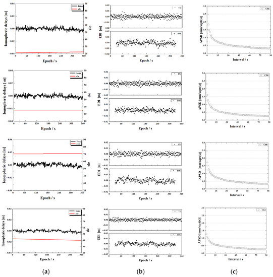
Figure 1.
Time series of satellite ionospheric delays (a), the EDI at a differential interval of 1 s and 60 s (b), and APSD obtained at a different differential interval (c) for satellite C01, C06, C08 and C12 (from top to bottom) of the zero-baseline. The sampling rate of the observations is 1 s.
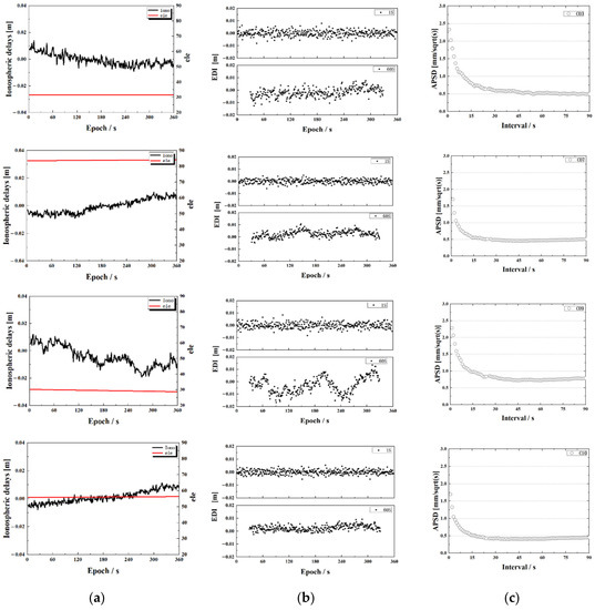
Figure 2.
Time series of satellite ionospheric delays (a), the EDI at a differential interval of 1 s and 60 s (b), and APSD obtained at a different differential interval (c) for satellite C03, C07, C09 and C10 (from top to bottom) of the long-range baseline of 202 km. The sampling rate of the observations is 1 s.
Compared to the ionospheric delay observations on the left column of the two baselines, the ionospheric delays are fully cancelled for the zero-baseline, although there are also small variations which are similar for all the satellites, indicating not the ionospheric delays but possibly a variation of inter-frequency bias. In the middle column, the EDI observations with 1 s and 60 s differential interval show that the 1 s time series is dominated by the observation noise, in the other words, the ionospheric delays change within 1 s is rather small compared with the observation noise, whereas the ionospheric variations show up in the plot with a 60 s interval. The APSDs of 1 s interval are almost the same of about 2 mm for all satellites over the two baselines because the APSD with the short differential interval reflects mainly the observation noises, which are almost the same for all satellites. The EDI with a 60 s interval for the zero-baseline shows also a similar but very small variation for all satellites which should be further investigated in the future.
Moreover, as can be seen from Figure 2, the ionospheric delays of the C09 satellite fluctuate greatly, and its APSD is also higher than that of other satellites. As is already mentioned, it is most likely due to the fact that the satellite has a low elevation over this period. This is also an indication of the necessity of using satellite-specified PSD.
From the time series of APSD in the right column, we can see that at the beginning (with a short differential interval) APSD is very large because of the observation noise, and then it degrades along with the interval increasing. For the long-range baseline, APSD becomes stable after a certain interval for example 30 s to 60 s but slightly different from satellite to satellite. For example, C09 needs a slightly larger interval which may be related to the higher ionospheric variations at a lower elevation. For the zero-baseline, because of no ionospheric delays in the ionospheric observations, its APSD keeps decreasing as it is reversely proportional to the differential interval.
Besides the impact of the differential interval, we also tested the effect of the number of samples used in the APSD calculation with Equation (23). We found that APSD is not very sensitive to the number of samples if it is larger than 30.
For one calculation of APSD with 1 Hz sampling rate, the total number of observations needed is the number of samples used plus the differential interval. For example, if we use 30 samples of EDI observations with a differential interval of 30 s and 60 s, about 60 and 90 observations are needed, respectively.
Based on these results, overall, we suggest that about 60 s to 90 s of carrier-phase observations of a 1 Hz sampling rate is needed in order to get rid of the observation noise while using APSD to replace PSD.
3.3. Ionospheric Smoothing Method
As is discussed before, the ionospheric delays obtained from phase observations is greatly affected by the observation noise including the influence of the environment. The ionospheric delays variation could be smaller than the carrier phase observation noise within a short time, so that the PSD of the ionospheric delays process cannot be derived correctly.
Based on the relationship between the PSD of ionospheric, observation noise and the ionospheric observations in Equation (22), the PSD of ionospheric and observation noise can be separated by a linear fitting with the APSDs of different differential intervals as input which is called the linear fitting approach afterwards. The algorithm is straight forward with rigorous theoretical reasoning, however it can be simplified for practical application.
As is well known, the white noise can be removed by a low-pass filter, for example, the moving average approach. A window of a certain width of the number of epochs is chosen, and it starts from the beginning and moves epoch-by-epoch to the end of the dataset. For each window, the average of all the samples that fall inside is calculated as the denoised sample. Of course, quality control can be applied to the samples to exclude outliers. The window width should be carefully selected, as with too short a width the observation noise cannot be reduced well; otherwise, the temporal ionospheric delays variation will be smoothed out. Through the numerical investigation in Section 3.2, it is suggested to use 30 to 60 samples of EDI observations with a differential interval of 30 or 60 s to obtain stable APSD value, so 60 s should be an optimal smoothing window and will be used in this study. Of course, this value will be further evaluated in the experimental validation.
We apply the moving window smoothing with a window width of n sampling epochs to the ionospheric observations, so the denoised ionospheric observation at epoch can be written as:
According to the variance propagation law, the denoised observation has noise with an STD of of the original ones, i.e., about 1/8 for n = 64; it is reasonable to consider the denoised ionospheric delays free of noises. This smoothing is carried out for all the epochs and then the PSD of the ionospheric delays process can be calculated epoch-wise directly from a certain number of the denoised ionospheric observations nearby according to Equation (25).
In fact, the epoch-difference can be now formed between adjacent epochs, as the observation noise is smoothed out. For completeness of the algorithm, it should be mentioned that at the start of real-time positioning, an empirical one should be selected for positioning, since the smoothing requires a certain number of observations to obtain the first estimated PSD. Here, a loose constraint may be safer than a tight one, compared to the first fixed time of the experimental validation. Using a loose constraint will slightly delay the convergence, but a too-tight one will result in wrong fixing.
Figure 3 shows the obtained PSD by use of the linear fitting approach based on Equation (22) and the moving average approach.
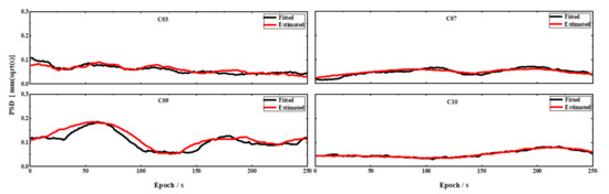
Figure 3.
The PSD obtained by the moving average approach and the PSD obtained by the linear fitting approach for satellite C03, C07, C09 and C10.
It can be seen from Figure 3 that the moving average approach can achieve almost the same PSD as the linear fitting approach, which is theoretically derived. This good agreement, on the one hand, confirms the theoretical derivation of the relationship between the PSD of ionospheric delays and observation noise in Section 3.2 and their separation. On the other hand, it shows the efficiency of the moving average approach in terms of both the accuracy and as well as the computational burden.
Taking the long baseline of 202 km as an example, the ionospheric observations obtained in Equation (11) and the smoothed ionospheric delays with Equation (24) for the selected satellites C03, C07, C09 and C10 are illustrated in Figure 4.
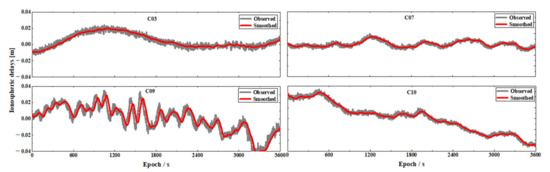
Figure 4.
Comparison of the observed ionospheric delays, smoothed ones with a moving window width of 60 s.
As illustrated in Figure 4, the residual ionospheric delays are at the level of a few centimeters in amplitude. The observed ones shown with the black dots are rather scattered and by using the smoothing method, the observation noise is removed significantly. The smoothed ionospheric delays show the relatively slow variation of the ionospheric observations. Therefore, the smoothed ionospheric delays can be used to quantify the real-time ionospheric changes for optimizing the constraint on the ionospheric delays parameters.
Figure 5 shows the correlation between EDI changes (black dots) and the calculated PSD (red line). The test result here and that in Section 4.5 suggest that about 60–90 s data of 1 Hz sampling rate is needed in order to get rid of the observation noise while using APSD to replace PSD. As illustrated in Figure 5, EDI is an indicator of the size of the ionospheric delays in epoch-difference, and PSD will also be adjusted accordingly with the ionospheric delays change, showing a positive correlation with the absolute amount of EDI. When the ionospheric delays change drastically and the corresponding EDI is large, the PSD will also increase. When the EDI is stable, the PSD will also be stable. Figure 5 can clearly demonstrate that the PSD change with the EDI.
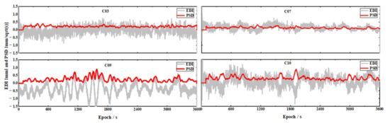
Figure 5.
Correlation between EDI and PSD.
4. Experimental Validation
4.1. Experimental Data
In total, three baselines from different networks are available for validating the efficiency of this proposed ionospheric constraint method. The baseline length, observation period, geographical location and receiver types are listed in Table 3. Baseline A is from the CORS network in Zhejiang Province at a low latitude, and Baseline B and Baseline C belong to the CORS network in Heilongjiang Province at a high latitude. All the receivers are capable of tracking BDS triple-frequency signals and the sampling rate is 1 Hz.
Table 3.
Information of baselines employed in the experimental validation.
4.2. Data Processing
The main purpose of the experimental validation is to investigate the efficiency of the proposed ionospheric constraint by the positioning performance in terms of the first ambiguity fixing time (FAFT) and positioning accuracy compared with traditional approaches. FAFT is the time when the station coordinates in three direction converge to 0.1 m. For the empirical PSD, although most of the studies use a fixed value, several values will be tested for each baseline and the best one will be used for a fair comparison, while in the proposed approach the satellite-specific PSD is estimated using ionospheric observations and the width of the smoothing window will also be tested. Therefore, we have here three processing schemas: (1) using the same Empirical PSD for all satellites and all epochs, referred to as EMP; (2) using Estimated satellite-specific PSD, named as EST; (3) using Estimated satellite-specific PSD with different smoothing window widths. Besides which, in this study, we focus on the long-range triple-frequency RTK, therefore only BDS triple frequency data are processed and the conclusions should be applicable to the other system.
The data of each baseline are divided into one-hour sessions and processed independently using the above-mentioned processing schemas. For each one-hour session, triple frequency data are processed in kinematic mode and integer ambiguity fixing is carried out using the strategy presented by Zhu et al. [34]. The FAFT, the estimated station coordinates and ionospheric delays are also derived and analyzed for each schema and baseline. Finally, the best processing strategy is applied to the static and kinematic processing of the three baselines and the statistics of the FAFT and positioning accuracy are presented.
4.3. Empirical Ionospheric Constraint
The processing using the different empirical PSD of 2.00, 1.00, 0.50, 0.20, 0.10 and 0.02 are carried out and statistics are derived for comparison. Taking Baseline C of 24-h data as an example, there are, in total, 24 one-hour sessions; the statistics of the FAFT and the positioning accuracy for the selected PSD are instructed in Table 4 and the result using the estimated satellite-specific constraint from 4.4 is also listed for comparison.
Table 4.
The FAFT and positioning accuracy of Baseline C with different empirical PSD.
From the statistics in Table 4, the results of the six different EMP constraints show that the best result in terms of the FAFT and positioning accuracy is achieved with the PSD of 0.50 , and with larger and smaller PSDs the performance is degraded. The results with the PSD of 0.20 and 0.50 are almost the same and they are very close to the EST60 processing schema with a slight degradation of about 8% in both the FAFT and positioning accuracy.
The position difference time series of the solution with the best and smaller and larger PSD are also illustrated in Figure 6. For clearance of the FAFT, the EST60 solution is also depicted for comparison. From Figure 6, the EST60 constraint has the fastest FAFT and stable position estimates after convergence. The EMP with 0.50 has almost the same performance. However, when the PSD of 0.02 is used, the FAFT are clearly delayed although the positioning accuracy does not decrease. We have also tested with even smaller PSD for example 0.005 , then the ambiguity cannot be fixed correctly and no reliable fixed solution is available. In principle, a loose constraint would be safer than a tight one if there is not reliable information.
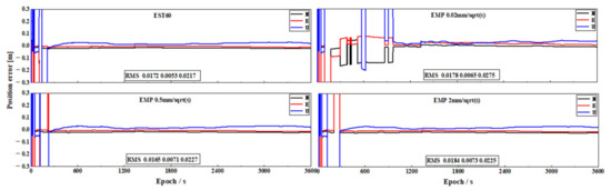
Figure 6.
Position differences with different PSD, including EST60, the best EMP value 0.5, EMP 0.02, and EMP 2 .
In order to further understand the impact of the different PSDs, the estimated ambiguities of their float solutions are instructed in Figure 7. It can be seen that the estimated ambiguities of the EMP 0.5 show similar behavior to the EST60 with high accuracy from the beginning, while the ambiguities of the EMP with 0.02 approach reach their stable status rather slowly and even with some slow fluctuations.
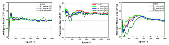
Figure 7.
The estimated ambiguities of the float solutions with the ionospheric delays PSD of EST60, 2 , 0.5 , and 0.02 .
Furthermore, we plot the estimated ionospheric delays for C07, C10, C12 from solutions with the EMP and EST power densities with the observed ionospheric delays as background in Figure 8.
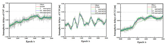
Figure 8.
The observed ionospheric delays and the estimated Ionospheric delays of the solutions with EMP and EST60 power densities. Only the estimates with fixed ambiguity are included.
As can be seen from Figure 8, with different ionospheric delay constraints, the overall trends of the ionospheric delays do not differ very much, but the short-term variation is underestimated along with the decrease meant of the power density. The difference of ionospheric delays between the EST60 constraint and EMP with 0.5 is the smallest.
4.4. Satellite-Specified Ionospheric Contraint
From the analysis in Section 4.3, the ionospheric constraint plays an important role in long-range RTK positioning. The PSD which decides the constraint depends on the baseline length and the ionospheric activity, therefore it is not easy to obtain a suitable empirical value, especially for real-time positioning. The proper way is to estimate the PSD from ionospheric observation itself as described in Section 3.3.
We use a window of 60 s to calculate the moving average of the observed ionospheric delays with simple quality control. The latest 30 smoothed ionospheric observations used to calculate the PSD at the current epoch are calculated for each satellite, so the constraint is satellite-specific instead of the same for all satellites. For comparison, the solutions with the estimated PSD scaled by 1/3 three times are also derived.
Similarly, the statistics of the 24 one-hour sessions of Baseline C are given in Table 5. In the comparison of the previous subsection, EST60 is confirmed superior to the best empirical constraint because its PSD derived from real data and the smoothing window width of 60 s is also proved to be the best in the following subsection. Here we further demonstrate that it is the best because both increasing or decreasing the PSD led to worse FAFT and positioning accuracy.
Table 5.
The FAFT and the Positioning Precision of Baseline C with the estimated PSD.
To show the impact of the constraint on the convergence, the estimated position time series, and ambiguity time series of C07, C10 and C12 for the solutions with EST60, EST60 × 3 and EST60 ÷ 3 are illustrated in Figure 9 and Figure 10, respectively.
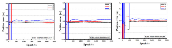
Figure 9.
Positioning results of EST60, EST60 × 3 and EST60 ÷ 3.
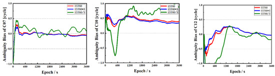
Figure 10.
The float ambiguity estimated of C07, C10 and C12 for the solution EST60, EST60 × 3 and EST60 ÷ 3.
In Figure 9, from left to right, the results of FAFT and positioning accuracy after the EST60 constraint, EST60 constraint enlarged by three times (EST60 × 3) and EST60 constraint enlarged by 0.3 times (EST60 ÷ 3), are shown, respectively. With the EST60 constraint, the FAFT becomes fast, and the results are good in E and N directions after convergence. After the EST60 constraint is enlarged 3 times and 0.3 times, FAFT slows down, respectively, which is due to the inappropriate PSD of the ionospheric delays constraint. Figure 10 shows the floating solutions of ambiguity of C07, C10 and C12 under the EST60, EST60 × 3 and EST60 ÷ 3 constraint.
When the EST60 is increased to EST60 × 3, the FAFT becomes slow, and the floating solutions are stable within the range of 0.5 m after convergence; when EST60 is reduced to EST60 ÷ 3, it takes a long time for the ambiguity residual to converge to a certain accuracy and fluctuates sharply up and down, so the ambiguity cannot be fixed and the positioning results are poor. On the contrary, the performance of the EST60 is much better than the former two, with a faster FAFT and more accurate positioning.
Figure 11 shows the corresponding fluctuation of ionospheric delays for C07, C10 and C12. EST60 estimates agree with the observed values perfectly which are almost in the middle of the observed ones. With the increased PSD of EST60 × 3, the ionospheric delays are close to that of EST60. With the decreased PSD of EST60 ÷ 3, the estimated ionospheric delays are overall underestimated, which are behind the observed values and in general cannot reflect the ionosphere delays variation, especially for sharp fluctuations.
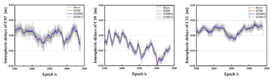
Figure 11.
The ionospheric delays time series of C07, C10 and C12 from the solution EST60, EST60 × 3 and EST60 ÷ 3.
4.5. Impact of the Smoothing Window Width
The moving average smoothing approach helps to reduce the influence of carrier observation noise and is conducive to the real reaction of ionospheric delays changes. The width of the window is very crucial, as too wide a width will also remove the ionospheric variation and too narrow a width cannot remove the noise adequately. In order to get the proper window width, a numerical test is undertaken using different window widths from 0 to 150 with a stepsize of 30 s, i.e., six windows. The window width 1 means using the original observations without any smoothing. The same statistics as in the previous subsections are used for evaluation. Again, taking Baseline C with 24 one-hour sessions as an example, the statistical results are shown in Table 6.
Table 6.
The FAFT and positioning accuracy using the PSD estimated with different smoothing window widths.
From the statistics in Table 6, the solution with a smooth window of 60 s is the best. Both the FAFT and positioning accuracy are degraded but very gently with larger and smaller windows. In principle, the difference for the window width from 30 s to 120 s is rather small, so that the selection of the window width should be not very difficult. In this study, 60 s is applied for all the sessions and baselines.
Similar to the investigation in Section 4.3 and Section 4.4, the similar performance of the position-biases, ambiguity convergence time and the estimated ionospheric delays of the solutions also shown in Table 6. Therefore, we will not repeat them here again.
The time series of EDI and PSD used in EST60 and that are calculated without smoothing, i.e., EST01 are illustrated in Figure 12 for satellite C07, C10 and C12.
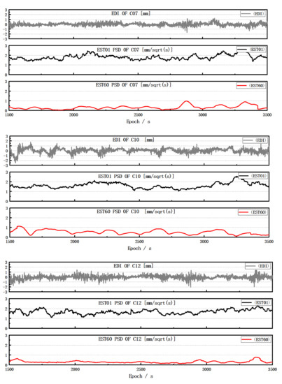
Figure 12.
The time series of EDI and estimated PSD used in EST01 and EST60 for satellite C07, C10 and C12 from top to bottom.
It can be seen from Figure 12 that the EST01 is affected by observation noise and exhibits much larger noise and cannot reflect the trend of the ionosphere delays in comparison with EST60 obtained by moving average approach. For example, the C07 has two large changes around the epochs 2700 and 3400, respectively, which can also be seen from the ionospheric delays time series in Figure 11. The PSD of EST60 is in good agreement with the ionospheric variation and can capture them precisely in real-time operation.
4.6. BDS Triple-Frequncy Long-Range RTK
The triple-frequency observations increase the redundancy of the estimation and can speed up the integer ambiguity resolution due to the constraint among the integer ambiguities of different frequencies. One of the critical issue is the modelling of the ionospheric delays. Here, the estimation model by Equations (5)–(8) with the constraint based on the estimated PSD is adopted to carry out the BDS triple-frequency positioning of Baselines A, Baseline B and Baseline C in static and kinematic mode. The PSD of the ionospheric delays is calculated from the latest 30 epochs of denoised ionospheric observations smoothing with the best window width of 60 s. For each baseline, four 2-h sessions are processed and the FAFT and positioning accuracy are calculated and listed in Table 7 and the number of satellites observed and positioning differences are shown in Figure 13.
Table 7.
The RMS statistical results of Baseline A, Baseline B and Baseline C.
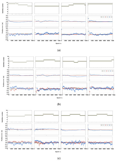
Figure 13.
The positioning results for Baselines A (a), Baseline B (b) and Baseline C (c). In each row, there are four subplots representing four 2-hour sessions. In each subplot, the top panel shows the number of satellites observed and the middle and bottom panel for the position differences in static and kinematic mode, respectively.
In Figure 13, the positioning results of Baseline A, Baseline B and Baseline C are shown on the top, middle and bottom row, respectively. In each row, there are four subplots each for one 2-h session. In each subplot, the upper panel presented the number of observed satellites, and the middle and bottom panel are for the position differences in E, N and U directions in static and kinematic mode, respectively. It can be seen from Figure 13 that the positioning result is stable after convergence, and the FAFT and positioning accuracies in kinematic mode are worse than those in static mode.
From the statistics in Table 7, it is indicated that the positioning accuracy of rover stations in both static and kinematic mode can reach the centimeter level. The longest and the shortest FAFT are 278 s and 217 s in static mode, and 302 s and 250 s in kinematic mode. The average FAFT are 226 s in the static mode, and 270 s in the kinematic mode. It can be seen from Figure 13 and Table 7 that the approach for estimating PSD proposed in this study can efficiently fix the integer ambiguity within 5 min and stabilize the rover station positioning results in both the static and kinematic mode.
5. Conclusions
For long-range precise positioning, instead of ionosphere-free observation, the un-combined observations are suggested, especially for triple-frequency data processing, in which the ionospheric delays are generally estimated as a random walk process with proper spatiotemporal constraint represented by the process PSD. Due to the ionospheric delays, variation depends on the inter-station distance and the ionosphere activities, and it is difficult to give a reasonable empirical PSD. The ionospheric delays derived from the phase observations containing the actual ionospheric delays variation, however, it is contaminated by the observation noise which is much larger than ionospheric variation in a very short time.
In this study, we deduced the relationship among the ionospheric delays PSD, observation noise and the ionospheric observations and demonstrated the impact of the observation noise in the estimation of the PSD and its reduction with increased differential interval.
Based on the numerical investigation, we developed two approaches to estimate the PSD: the linear fitting approach with rigorous theoretical reasoning and the moving average approach which is more efficient for real-time processing. The influence of the window width, and the sampling and differential interval are carefully investigated and proper values are suggested based on the experimental data, for example with a smooth window of 60 s and epoch-differenced ionospheric observations of 30 s for the observations of 1 Hz.
In the experimental validation, the results show that both the FAFT and positioning accuracy after ambiguity fixing using the estimated PSD as a constraint can be increased by at least 8% compared with that using the unique empirical value for all satellites, although the value is fine-tuned according to the actual observations, and decreased by 34% compared to that using PSD calculated without smoothing.
The proposed approach is employed in the processing of BDS triple-frequency data of three long-range baselines of 103 km, 175 km and 202 km to validate the positioning performance in terms of the FAFT and positioning accuracy. The average FAFT in static and kinematic mode is 226 s and 270 s, and the positioning accuracies after ambiguity fixing are 1 cm, 1 cm and 3 cm and 3 cm, 3 cm and 6 cm in the East, North and Up directions for static and kinematic mode, respectively. The accuracy shows a slight correlation with inter-station distance and meets the requirements of high-precision static and kinematic positioning.
Author Contributions
H.Z. conceived the idea and designed the experiments with A.X., M.G., H.Z. and J.L. wrote the main manuscript. A.X., M.G., L.T. and J.L. reviewed the paper. All components of this research were carried out under the supervision of H.Z. and M.G. All authors have read and agreed to the published version of the manuscript.
Funding
This research was funded by the National Natural Science Foundation of China (Grant Nos. 42030109, 42074012), The Liaoning Key Research and Development Program (No. 2020JH2/10100044), and The National Key Research and Development Program (No. 2016YFC0803102).
Institutional Review Board Statement
Not applicable.
Informed Consent Statement
Not applicable.
Acknowledgments
The authors gratefully acknowledge the Zhejiang and Heilongjiang CORS network for providing the multi-GNSS data.
Conflicts of Interest
The authors declare no conflict of interest.
References
- Dubey, S.; Wahi, R.; Gwal, A.K. Ionospheric effects on GPS positioning. Adv. Space Res. 2006, 38, 2478–2484. [Google Scholar] [CrossRef]
- Mageed, K. Accuracy assessment for processing GPS short baselines using ionosphere-free linear combination. Aust. J. Basic Appl. Sci. 2011, 5, 793–800. [Google Scholar]
- Bock, Y.; Sergei, A. Gourevitch, Counselman, Charles C., III, Interferometric analysis of GPS phase observations. Manuscr. Geod. 1986, 11, 282–288. [Google Scholar]
- Schaffrin, B.; Bock, Y. A unified scheme for processing GPS dual-band phase observations. Bull. Géod. 1988, 62, 142–160. [Google Scholar] [CrossRef]
- Shen, Y.Z.; Xug, C. Simpilified Equivalent Represtation of GPS Observation Equations. GPS Solut. 2007, 12, 99–108. [Google Scholar] [CrossRef]
- Yang, Y.; Mao, Y.; Sun, B. Basic performance and future developments of BeiDou global navigation satellite system. Satell. Navig. 2020, 1, 1. [Google Scholar] [CrossRef] [Green Version]
- Geng, J.; Guo, J.; Meng, X.; Gao, K. Speeding up PPP ambiguity resolution using triple-frequency GPS/BeiDou/Galileo/QZSS data. J. Geod. 2020, 94, 1–15. [Google Scholar] [CrossRef] [Green Version]
- Qin, H.; Liu, P.; Cong, L.; Ji, W. Triple-Frequency Combining Observation Models and Performance in Precise Point Positioning Using Real BDS Data. IEEE Access 2019, 7, 69826–69836. [Google Scholar] [CrossRef]
- Tu, R.; Zhang, H.; Ge, M.; Huang, G. A real-time ionospheric model based on GNSS Precise Point Positioning. Adv. Space Res. 2013, 52, 1125–1134. [Google Scholar] [CrossRef]
- An, X.; Meng, X.; Jiang, W. Multi-constellation GNSS precise point positioning with multi-frequency raw observations and dual-frequency observations of ionospheric-free linear combination. Satell. Navig. 2020, 1, 7. [Google Scholar] [CrossRef]
- Klobuchar, J.A. Ionospheric Time-Delay Algorithm for Single-Frequency GPS Users. IEEE Trans. Aerosp. Electron. Syst. 1987, AES-23, 325–331. [Google Scholar] [CrossRef]
- Basile, F.; Moore, T.; Hill, C.; McGraw, G.; Johnson, A. Multi-Frequency Precise Point Positioning using GPS and Galileo data with smoothed ionospheric corrections. In Proceedings of the 2018 IEEE/ION Position, Location and Navigation Symposium (PLANS), Monterey, CA, USA, 23–26 April 2018; IEEE: Piscataway, NJ, USA, 2018; pp. 1388–1398. [Google Scholar]
- Zhang, H.; Han, W.; Huang, L.; Geng, C. Modeling global ionospheric delay with IGS ground-based GNSS observations. Wuhan Daxue Xuebao (Xinxi Kexue Ban)/Geomat. Inf. Sci. Wuhan Univ. 2012, 37, 1186–1189. [Google Scholar]
- Li, Z.; Yuan, Y.; Wang, N.; Hernandez-Pajares, M.; Huo, X. SHPTS: Towards a new method for generating precise global ionospheric TEC map based on spherical harmonic and generalized trigonometric series functions. J. Geod. 2015, 89, 331–345. [Google Scholar] [CrossRef]
- Teunissen PJ, G.; Odijk, D.; Zhang, B.C. PPP-RTK: Results of CORS Network-Based PPP with Integer Ambiguity Resolution. J. Aeronaut. Astronaut. Aviat. Ser. A 2010, 42, 223–229. [Google Scholar]
- Odijk, D.; Teunissen, P.J.G. Improving the speed of CORS Network RTK ambiguity resolution. In Proceedings of the IEEE Position Location & Navigation Symposium, Indian Wells, CA, USA, 4–6 May 2010; IEEE: Piscataway, NJ, USA, 2010; pp. 79–84. [Google Scholar]
- Teunissen, P.J.G. The geometry-free GPS ambiguity search space with a weighted ionosphere. J. Geod. 1997, 71, 370–383. [Google Scholar] [CrossRef] [Green Version]
- Wielgosz, P. Quality assessment of GPS rapid static positioning with weighted ionospheric parameters in generalized least squares. GPS Solut. 2010, 15, 89–99. [Google Scholar] [CrossRef]
- Bock, Y. Medium-distance GPS measurements. In GPS for Geodesy, Lecture Notes in Earth Sciences; Kleusberg, A., Teunissen, P.J.G., Eds.; Springer: Berlin/Heidelberg, Germany; New York, NY, USA, 1996; Volume 60, Chapter 9. [Google Scholar]
- Teunissen, P.J.G. The ionosphere-weighted GPS baseline precision in canonical form. J. Geod. 1998, 72, 107–117. [Google Scholar] [CrossRef]
- Goad, C.C.; Ming, Y. A new approach to precision airborne GPS positioning for photogrammetry. Photogramm. Eng. Remote Sens. 1997, 63, 1067–1077. [Google Scholar]
- Odijk, D. Weighting Ionospheric Corrections to Improve Fast GPS Positioning Over Medium Distances. In Proceedings of the 13th International Technical Meeting of the Satellite Division of the Institute of Navigation, Salt Lake City, UT, USA, 19–22 September 2000; Institute of Navigation: Manassas, VA, USA, 2000; pp. 1113–1123. [Google Scholar]
- Tang, W.; Liu, W.; Zou, X.; Li, Z.; Shi, C. Improved ambiguity resolution for URTK with dynamic atmosphere constraints. J. Geod. 2016, 90, 1359–1369. [Google Scholar] [CrossRef]
- Zou, X.; Wang, Y.; Deng, C.; Li, Z.; Shi, C. Instantaneous BDS + GPS undifferenced NRTK positioning with dynamic atmospheric constraints. GPS Solut. 2018, 22, 17. [Google Scholar] [CrossRef]
- Zhang, M.; Liu, H.; Bai, Z.; Qian, C.; Fan, C.; Zhou, P.; Shu, B. Fast ambiguity resolution for long-range reference station networks with ionospheric model constraint method. GPS Solut. 2017, 21, 617–626. [Google Scholar] [CrossRef]
- Shi, C.; Gu, S.; Lou, Y.; Ge, M. An improved approach to model ionospheric delays for single-frequency Precise Point Positioning. Adv. Space Res. 2012, 49, 1698–1708. [Google Scholar] [CrossRef]
- Zhao, Q.; Wang, Y.T.; Gu, S.; Zheng, F.; Shi, C.; Ge, M.; Schuh, H. Refining ionospheric delay modeling for undifferenced and uncombined GNSS data processing. J. Geod. 2019, 93, 545–560. [Google Scholar] [CrossRef]
- Albashir, A.; Sami, K. Enhancing The Accuracy of GPS Point Positioning by Modeling the Ionospheric Propagation Delay. In Proceedings of the 2018 International Conference on Computer, Control, Electrical and Electronics Engineering (ICCCEEE), Khartoum, Sudan, 12–14 August 2018; IEEE: Piscataway, NJ, USA, 2008; pp. 1–7. [Google Scholar]
- Liu, G.C.; Lachapelle, G. Ionosphere weighted GPS cycle ambiguity resolution. In Proceedings of the ION NTM 2002, San Diego, CA, USA, 28–30 January 2002; Institute of Navigation: Manassas, VA, USA, 2002; pp. 889–899. [Google Scholar]
- Schaer, S.; Beutler, G.; Rothacher, M.; Brockmann, E.; Wild, U. The impact of the atmosphere and other systematic errors on permanent GPS networks. In Geodesy Beyond 2000; Springer: Berlin/Heidelberg, Germany, 2000. [Google Scholar]
- Pi, X.; Mannucci, A.J.; Lindqwister, U.J.; Ho, C.M. Monitoring of global ionospheric irregularities using the Worldwide GPS Network. Geophys. Res. Lett. 1997, 24, 2283–2286. [Google Scholar] [CrossRef]
- Böhm, J.; Niell, A.; Tregoning, P.; Schuh, H. Global Mapping Function (GMF): A new empirical mapping function based on numerical weather model data. Geophys. Res. Lett. 2006, 33. [Google Scholar] [CrossRef] [Green Version]
- Ge, M.; Gendt, G.; Dick, G.; Zhang, F.P.; Rothacher, M. A New Data Processing Strategy for Huge GNSS Global Networks. J. Geod. 2006, 80, 199–203. [Google Scholar] [CrossRef]
- Zhu, H.; Lu, Y.; Tang, L.; Li, J.; Ge, M. A Comparative Study of BDS Triple-Frequency Ambiguity Fixing Approaches for RTK Positioning. Sensors 2021, 21, 2565. [Google Scholar] [CrossRef]
- Teunissen, P.J.G. An optimality property of the integer least-squares estimator. J. Geod. 1999, 73, 587–593. [Google Scholar] [CrossRef]
- Davies, K.; Hartmann, G.K. Studying the ionosphere with the Global Positioning System. Radio Sci. 2016, 32, 1695–1703. [Google Scholar] [CrossRef]
- Komjathy, A. Global Ionospheric Total Electron Content Mapping Using the Global Positioning System. Ph.D Thesis, University of New Brunswick, Fredericton, NB, Canada, 1997. [Google Scholar]
Publisher’s Note: MDPI stays neutral with regard to jurisdictional claims in published maps and institutional affiliations. |
© 2021 by the authors. Licensee MDPI, Basel, Switzerland. This article is an open access article distributed under the terms and conditions of the Creative Commons Attribution (CC BY) license (https://creativecommons.org/licenses/by/4.0/).