Estimating the Key Parameter of a Tropical Cyclone Wind Field Model over the Northwest Pacific Ocean: A Comparison between Neural Networks and Statistical Models

Abstract

Estimation of maximum wind speed associated with tropical cyclones (TCs) is crucial to evaluate potential wind destruction. The Holland B parameter is the key parameter of TC parametric wind field models. It plays an essential role in describing the radial distribution characteristics of a TC wind field and has been widely used in TC disaster risk evaluation. In this study, a backpropagation neural network (BPNN) is developed to estimate the Holland B parameter ($B_s$) in TC surface wind field model. The inputs of the BPNN include different combinations of TC minimum center pressure difference ($\Delta p$), latitude, radius of maximum wind speed, translation speed and intensity change rate from the best-track data of the Joint Typhoon Warning Center (JTWC). We find that the BPNN exhibits the best performance when only inputting TC central pressure difference. The $B_s$ estimated from BPNN are compared with those calculated from previous statistical models. Results indicate that the proposed BPNN can describe well the nonlinear relation between $B_s$ and $\Delta p$. It is also found that the combination of BPNN and Holland’s wind pressure model can significantly improve the maximum wind speed underestimation and overestimation of the two existing wind pressure models (AH77 and KZ07) for super typhoons.

1. Introduction

The Northwest Pacific (NWP) Ocean is one of the most cyclone-prone regions worldwide. Tropical cyclones (TCs) can cause serious meteorological disasters, such as strong winds and heavy rainfall and result in severe damage to the coastal provinces of Southeast China, Philippines and Japan, affecting the safety of the lives and properties of their residents. Therefore, it is crucial to carry out the risk assessment of TC-induced potential hazards, including intense winds, storm surges and torrential rain.

Due to the lack of high-quality in situ observations of TCs in the coastal areas of China, it is inappropriate to conduct TC risk evaluation only based on historical data alone. However, the parametric wind field model of TCs has the advantages of straightforward form, simple calculation and relatively accurate simulation of the essential characteristics of the TC structure. TC two-dimensional wind fields can be constructed with the parametric wind field model by inputting key parameters, such as radial wind profile shape parameter (Holland $B_s$), minimum central pressure (MCP), radius of maximum wind speed (RMW), azimuth angle of maximum wind speed and TC translation speed. TC surface wind fields have been widely used in evaluating TC disaster risk and forecasting storm surges.

The TC wind pressure model links the minimum central surface pressure and the maximum wind speed (MWS) near the TC center. It is an important analysis tool to evaluate the MWS from various observations and estimates. Basically, all kinds of wind pressure models are developed in the same equation form (Equation (1), [1]):

$$V_m=\alpha \Delta P^x$$

(1)

where $V_m$ is the maximum wind speed and $\Delta P$=$P_n‐P_c$ is the difference between the environmental pressure $P_n$ and the pressure of the TC center $P_c$. The value of $P_n$ in the NWP is usually 1010 hPa and α and x are empirical constants. Many scholars have adjusted the values of these two empirical constants based on this form. Atkinson and Holliday [2] adopted an empirical method to define the exponents of the wind pressure model for different cyclone-prone basins (AH77 model):

$$V_m=3.4(1010‐P_c{)}^{0.644}$$

(2)

$$V_m=3.92(1015‐P_c{)}^{0.644}$$

(3)

where $V_m$ is the one min average wind speed at a height of 10 m, 1010 is an assumed environmental pressure constant for the NWP and 1015 corresponds to the situation in the North Atlantic.

Knaff and Zehr [3] reclassified the data used in the AH77 model according to different intensities and, thus, to remove a bias of a large number of weaker intensities existing in the samples. The new empirical values of the wind pressure model were calculated as follows (KZ07 model):

$$V_m=2.3(1010‐P_c{)}^{0.76}$$

(4)

The TC pressure field is an essential component of many parametric wind field models. Schloemer [4] proposed an exponential pressure distribution model as follows:

$$P(\mathrm{r})=P_c+\Delta P{\mathrm{e}}^{[-(\frac{\mathrm{RMW}}{\mathrm{r}})]}$$

(5)

where $P(\mathrm{r})$ is the value of pressure at distance r between the observation point and the TC center.

On the basis of the pressure field model mentioned above, Holland [5] introduced a parameter B to exhibit variation of pressure gradient at the RMW which is referred to as the H80 model hereafter.

$$P(\mathrm{r})=P_c+(P_n‐P_c){\mathrm{e}}^{-{(\frac{\mathrm{r}}{\mathrm{RMW}})}^B}$$

(6)

where B is the Holland B parameter, which defines the shape of the TC pressure profile.

The wind profile and the MWS are expressed by using the gradient wind equations. Here, the Coriolis force term was ignored.

$$V_c={[\frac{B\Delta P}{\rho }(\frac{\mathrm{RMW}}{\mathrm{r}}{)}^B{\mathrm{e}}^{{[-(\frac{\mathrm{RMW}}{\mathrm{r}})]}^B}]}^{\frac{1}{2}}$$

(7)

$$V_m=(\frac{B}{\rho \mathrm{e}}\Delta P{)}^{0.5}$$

(8)

where $\rho$ is the air density, e is the base of the natural logarithm function, r is the distance from the observation point to the TC center and$V_m$ is the maximum wind speed. Equations (7) and (8) can describe the TC radial wind profile and MWS at gradient height, but they need to be converted into ocean surface wind field information through the boundary layer model and certain errors occur during the transformation process.

The Holland B parameter is considered important to describe the radial distribution characteristics of the TC wind field, as discussed above. Figure 1 shows the examples of ocean surface pressure profiles and gradient wind speed profiles estimated from Equations (6) and (7) (both with the Holland B parameter). As shown in Figure 1a, for the same TC, that is, when $\Delta \mathrm{P}$ and RMW are fixed, as B increases, the pressure gradient increases significantly and is generally concentrated near the region of 1 RMW. In Figure 1b, with the increasing B value, the gradient wind speed near 1 time of RMW continues to increase, whereas the wind speed far away from the RMW continues to decrease.

Since Holland introduced the shape parameter of the wind profile in 1980 [5], many scientists have fitted corresponding Holland B parameter statistical models for different TC-prone basins. Love et al. [6] conducted an operational analysis of TCs in the northern ocean region of Australia. They found that the Holland B parameter obtained in this area has a weak logarithmic relationship with the TC central pressure difference. Hubbert et al. [7], Harper and Holland [8] focused on TCs in Australia and directly defined B as a linear function expression related to the TC central pressure. Vickery et al. [9] believed that B is related to the TC center pressure difference and RMW based on the aircraft reconnaissance data in the Atlantic Ocean and established a corresponding linear relationship. Willoughby and Rahn [10] used the same data as Vickery [9] to construct a statistical model of B, incorporating the flight-level maximum wind speed, latitude and RMW. According to the gradient balance equation, Jakobsen et al. [11] proposed a B model in the Bay of Bengal as a function of the TC central pressure difference and maximum wind speed.

In addition, previous studies found that the Holland B parameter is related to RMW and latitude [12,13]. Holland [14] developed a new correlation method between TC central pressure and MWS and further proposed a method to determine the value of the $B_s$ parameter objectively, which is directly related to the sea surface wind field (Holland08 model). The subscript of the parameter $B_s$ indicates that the relationship uses ocean surface data rather than the gradient wind field used in the original H80 model. The $B_s$ parameter relates the central pressure difference, intensity change rate, latitude and TC translation speed.

For the NWP, Xiao et al. [15] used historical typhoon data provided by the China Meteorological Administration (CMA) and the State Oceanic Administration to establish statistical models of B, which are related to the RMW for 11 major cities in the southeast coastal areas of China. Lin et al. [16] and Li et al. [17] compared the effects of different Holland B parameter models on the simulation results of the wind field in the NWP and determined that the model of Vickery [13] is most suitable for TC simulation in the NWP. Zhao et al. [18] used in situ atmospheric observation data from hundreds of national meteorological stations along the coast of China to build the expression of the Holland B parameter before and after typhoon landfall. Among them, B before landfall is related to the TC central pressure difference and RMW, whereas after landing, B is only related to the central pressure difference. Fang et al. [19] estimated a statistical model of the Holland $B_s$ parameter for landing TCs, using near-Earth environmental pressure data of hundreds of weather stations along the coast of the NWP and incorporating the central pressure difference and RMW. In addition, Fang et al. [20] adopted the TC position information and central pressure from the best-track dataset of CMA for the first time to propose a linear relationship between the Holland $B_s$ parameter and the central pressure difference and latitude (Fang2020 model).

Table 1. Summary of previously established Holland B or $B_s$ statistical models for different basins.

Serial Number	Formula	Research Area	Reference
(1)	$B=\mathit{0.25}+\mathit{0.3}\ln (\Delta P)$	Australia	1985 [6]
(2)	$B=\mathit{1.5}+(\mathit{980}-P_c)/\mathit{120}$	Australia	1991 [7]
(3)	$B=\mathit{2}-(P_c-\mathit{900})/\mathit{160}$	Australia	1999 [8]
(4)	$B=\mathit{1.38}-\mathit{0.00184}\Delta P+\mathit{0.00309}RMW$	Atlantic	2000 [9]
(5)	$\begin{array}{c}B=\mathit{1.0036}+\mathit{0.0173}{V}_{Fmax}+\mathit{0.0313}\ln (RMW)+\mathit{0.0087}\varnothing \end{array}$	Atlantic	2004 [10]
(6)	$B=\frac{\mathrm{e}}{{\gamma }_{\mathit{2}}^{\mathit{2}}}\frac{{\rho }_A}{\left[\mathit{100}\right]\Delta P}{(V_{max})}^{\mathit{2}}$	The bay of Bengal	2004 [11]
(7)	$B=\mathit{1.881}-\mathit{0.00557}RMW-\mathit{0.01097}\varnothing$	Atlantic	2005 [12]
(8)	$B=\mathit{1.881}-\mathit{0.00557}RMW-\mathit{0.01295}\varnothing$	Atlantic	2008 [13]
(9)	$\begin{array}{c}{B}_s=-\mathit{4.4}\times {\mathit{10}}^{-\mathit{5}}\Delta P^{\mathit{2}}+\mathit{0.01}\Delta P+\mathit{0.03}\frac{\partial P_c}{\partial t}-\mathit{0.014}\varnothing +\mathit{0.15}{V}_t^x+\mathit{1.0}\end{array}$ $x=\mathit{0.6}(\mathit{1}-\frac{\Delta P}{\mathit{215}})$ $B=B_s{(\frac{V_{mg}}{V_m})}^{\mathit{2}}\backsim \mathit{1.6}{B}_s$	Atlantic	2008 [14]
(10)	$\ln B=d_{\mathit{0}}+d_{\mathit{1}}\ln RMW+{\epsilon }_{\mathit{2}}$	NWP	2011 [15]
(11)	$B=-\mathit{2.365}+\mathit{0.0573}\Delta P+\mathit{0.0035}RMW$ (before landfall) $B=\mathit{0.4899}+\mathit{0.0178}\Delta P$ (after landfall)	NWP	2013 [18]
(12)	$\begin{array}{c}{B}_s=\mathit{4.1025}\times {\mathit{10}}^{-\mathit{5}}\Delta P^{\mathit{2}}+\mathit{0.0293}\times \Delta P+\mathit{0.7959}\times \ln RMW-\mathit{4.6010}\end{array}$ $\ln RMW=-\mathit{38.36}\Delta P^{\mathit{0.025}}+\mathit{46.75}+{\epsilon }_{\ln RMW}$	NWP	2018 [19]
(13)	$\begin{array}{c}{B}_s=\mathit{1.2858}+\mathit{8.6396}\times {\mathit{10}}^{-\mathit{3}}\Delta P-\mathit{8.7745}\times {\mathit{10}}^{-\mathit{3}}\varnothing \end{array}$	NWP	2020 [20]

lists the statistical models of Holland B or $B_s$ parameter established by the scholars mentioned above for different cyclone-prone basins. Among them, $\Delta P$ is the difference between the environmental pressure and the central pressure of the TC in hPa, $P_c$ is the TC central pressure in hPa, RMW is the RMW in km, $V_{Fmax}$ is the flight-level MWS in $m{s}^{-1}$, $\varnothing$ is the latitude of the TC center point in degrees, ${\gamma }_2=1.05$, ${\rho }_A$ is the air density and the value is 1.15 $kg{m}^{-3}$, $V_{max}$ is the MWS at 500 m above sea level,$(\partial p_c/\partial t)$ is the intensity change rate in $hPa{h}^{-1}$, $V_t$ is the TC moving speed in $m{s}^{-1}$, $V_{mg}/V_m$ is the surface-to-gradient wind transformation coefficient at RMW and $d_0,d_1$ are correlation coefficients (See Ref. [15] Table 5).

In accordance with previous studies [6,7,8,9,10,11,12,13,14,15,16,17,18,19,20], Holland B or $B_s$ parameter may be referred to TC central pressure, RMW, the latitude of the TC center location, TC translation speed and intensity change rate and it has various characteristics for different cyclone-prone basins. Almost all of the existing Holland B or $B_s$ parameter statistical models consider the linear relationship between the B or $B_s$ parameter and impact factors and only a few models consider the quadratic fitting relationship between $B_s$ and the TC central pressure difference. However, linear regression or simple quadratic fitting cannot fully explain the actual changes in the Holland B parameter. By contrast, backpropagation (BP) neural networks have a powerful nonlinear mapping ability and can deal with nonlinear processes flexibly. It can store the complex relationship between input variables and output results in the network through sample training and is an advantageous tool for building nonlinear models. In theory, as long as the number of neurons in the hidden layer is set enough, a BP neural network with three or more layers can approximate a nonlinear function with arbitrary accuracy. Therefore, a BP neural network can be used to establish a nonlinear model between the Holland B parameter and other impact factors.

Given the absence of aircraft reconnaissance in situ observation in the NWP, only a few studies on the Holland B parameter have been conducted in this basin [15,18,19,20]. The best-track dataset from the Joint Typhoon Warning Center (JTWC) has provided RMW data since 2001; such data can provide enough impact factor datasets for the simulation of the Holland B parameter in the NWP. Therefore, in this study, the JTWC best-track dataset is used for the first time to establish a BP neural network of the sea surface wind field Holland B parameter $B_s$ in the NWP and build a corresponding statistical model for comparison. Our main motivation is to develop an optimal model of the Holland $B_s$ parameter in the NWP and analyze its application.

Section 2 introduces the data used in this study, mainly including the best-track dataset of JTWC and the Soil Moisture Active and Passive (SMAP) TC sea surface wind field data. This section also introduces the quality control standards of the best-track dataset. Section 3 shows the definition method of sea surface wind field Holland B parameter and the structural configuration of the BP neural network used in this study. Section 4 describes the validation, application and comparison with statistical models of the neural network. Section 5 discusses the main advantages of the neural network applied to the wind pressure model. Section 6 provides the conclusions.

2. Data

2.1. JTWC Best-Track Data

This study adopts the TC best-track dataset in the NWP from 2001 to 2018 provided by the JTWC. Each best-track datum includes TC information, such as the basin where the TC is located; the annual TC number; the year, month, day and hour of TC occurrence; the longitude and latitude of the TC center location, the maximum one-minute continuous wind speed; the MCP; the TC intensity level, the RMW. The temporal resolution of the best-track dataset of JTWC is 6 h, which can be downloaded from the official website of JTWC (https://www.metoc.navy.mil/jtwc/jtwc.html accessed on 27 April 2020).

To ensure the validity of the final Holland B parameter model, this study first conducts quality control on the original JTWC best-track dataset. Thus, the quality control criteria (QCC) are defined as follows: (1) The central position of TCs is in the longitude range of 100°E–180°E and the latitude range is 0°–60°N. (2) The intensity of TCs is not less than 17.2 m/s. (3) The MCP of TCs is between 870 and 1000 hPa. (4) The RMW of TCs shall not exceed 150 km. (5) Landing TC data are removed. QCC -1 ensures that the TC best-track dataset used is located in the NWP. QCC-2 and QCC-3 ensure that the intensity of the TC best-track dataset reaches at least the tropical storm level because of too weak TCs having minimal research value. Given that the TCs with large RMW are generally weak and the peripheral wind field is extremely irregular, the final model results are affected to a certain extent. Therefore, we select the best-track dataset according to QCC-4, referring to the relevant literature [13]. Finally, QCC-5 is used to remove the landfall impact of TCs. The TC translation speed and intensity change rate can be calculated from the best-track dataset.

After quality control, we selected 6091 TC best-track data from the 2001–2018 JTWC dataset. Through random sampling, 80% of the dataset (4873 TC track data, hereafter called the training data) are selected to establish the model. The remaining 20% (1218 TC track data, hereafter called the testing data) are used for model testing. Figure 2 shows the geographical distribution density of the selected 4873 TC centers for the training data, indicating that TCs mainly occur in the longitude range of 110°E–140°E and the latitude range of 10°N–30°N. The distribution of the remaining 1218 TC centers for the testing data is also drawn on the Figure 2 with red hollow circles. It is clearly shown in Figure 2 that there is not much difference in the spatial distribution of the two sets of data.

For each selected best-track data, we extract information, such as MWS, MCP, RMW, latitude of the TC center position, translation speed and intensity change rate. The histograms of the key information contained in the training data samples used for modeling are shown in Figure 3. Figure 3a shows the intensity range of TC samples from $~$18–87 m/s, which ensures that the training data cover TCs from tropical storms to super typhoons. The range of other TC information is also shown in Figure 3b–f.

2.2. SMAP TC Sea Surface Wind Field Data

The NASA SMAP satellite observation station was launched in 31 January 2015 and began to provide data in April 2015. The L-band passive microwave radiometer mounted on the SMAP can be used to measure sea surface wind speed, with a spatial resolution of 40 km and a swath width of 1000 km. In addition, it has been proven that the L-band microwave radiometer performs well in observing the sea surface wind field of TCs [21,22,23]. A recent study [21] showed a good relationship between the wind-induced brightness temperature of the SMAP L-band microwave radiometer and the wind speed of TCs. The L-band microwave radiometer is not susceptible to rainfall attenuation even in extreme weather conditions and the brightness temperature consequently does not reach saturation. Therefore, it can provide an accurate estimate of TC intensity, which arrives at super typhoon grade. The SMAP wind field data with a spatial resolution of 0.25° × 0.25° used in this study are from the remote sensing system website (www.remss.com/missions/SMAP/ accessed on 10 November 2020).

To discuss the applicability of the network further (see Section 5), we select 26 TCs with super typhoon grade in the NWP Ocean from April 2015 to December 2019, totaling 48 SMAP sea surface wind field observation samples.

Table 2. Information on super typhoons observed by SMAP from 2015 to 2019.

Year	Name of Super Typhoons	Occurrence Time of Super Typhoons Observed by SMAP	MWS of Super Typhoons Extracted Directly from SMAP Wind Field Data (m/s)
2015	Noul	9 May 2015-09:50	56.94
	Noul	9 May 2015-22:00	73.61
	Dolphin	15 May 2015-20:46	54.52
	Nangka	9 July 2015-08:00	61.52
	Soudelor	3 August 2015-08:35	60.28
	Soudelor	3 August 2015-20:44	74.02
	Soudelor	7 August 2015-09:27	56.68
	Atsani	18 August 2015-20:07	54.26
	Dujuan	27 September 2015-09:40	64.50
	Dujuan	27 September 2015-21:46	59.36
	Champi	22 October 2015-20:44	51.69
	In-fa	21 November 2015-21:12	51.44
	Melor	13 December 2015-21:36	54.68
2016	Nepartak	5 July 2016-21:22	70.42
	Nepartak	6 July 2016-21:58	70.67
	Meranti	12 September 2016-09:02	73.45
	Malakas	16 September 2016-21:59	61.36
	Chaba	2 October 2016-21:58	62.60
	Chaba	4 October 2016-09:30	55.96
	Songda	12 October 2016-19:51	51.28
	Haima	17 October 2016-21:23	59.10
	Haima	18 October 2016-22:00	68.87
2017	Noru	31 July 2017-08:37	53.85
	Lan	22 October 2017-08:52	61.05
2018	Maria	7 July 2018-08:23	63.06
	Maria	8 July 2018-09:00	66.46
	Maria	8 July 2018-21:07	70.16
	Jebi	1 September 2018-08:24	70.36
	Jebi	2 September 2018-21:06	55.55
	Jebi	3 September 2018-21:41	53.65
	Mangkhut	13 September 2018-09:10	77.93
	Mangkhut	13 September 2018-21:22	69.08
	Mangkhut	14 September 2018-09:49	67.43
	Trami	24 September 2018-21:33	62.65
	Trami	29 September 2018-09:14	52.77
	Kong-rey	1 October 2018-08:47	51.80
	Yutu	24 October 2018-08:10	68.62
	Yutu	24 October 2018-20:20	61.62
	Yutu	25 October 2018-20:57	65.94
	Yutu	28 October 2018-09:00	67.95
	Yutu	29 October 2018-09:37	59.72
2019	Wutip	24 February 2019-08:21	51.59
	Wutip	24 February 2019-20:33	53.85
	Wutip	25 February 2019-21:09	56.12
	Lingling	6 September 2019-09:39	51.02
	Bualoi	22 October 2019-08:22	64.81
	Bualoi	22 October 2019-20:30	56.63
	Bualoi	24 October 2019-08:00	56.73

summarizes the year, name, occurrence time of each TC and the corresponding MWS information extracted directly from the SMAP wind field data.

3. Methodology

3.1. Definition of Holland B Parameter for Sea Surface Wind Field

To develop the model of Holland B parameter, this study considers the TC central pressure difference $(\Delta P$ =$P_n‐P_c)$, RMW, latitude ($\varnothing$), motion speed$(V_{storm})$ and intensity change rate$(\partial p_c/\partial t)$ as alternative independent variables. Among them, the value of environmental pressure $P_n$ is defined as 1010 hPa (the research basin is considered to be the NWP). Although $P_n$ is best used as a variable, no corresponding $P_n$ value exists in most best-track datasets. Thus, using $P_n$ as a fixed value for different basins is also helpful for the convenience of subsequent model application. In addition, other alternative variables can be obtained directly or calculated indirectly from the JTWC best-track dataset.

Holland [14] combined Equation (8) with the ideal gas state equation and deduced the Holland B parameter $B_s$, which is directly related to the sea surface wind field.

$$B_s=\frac{V_{max}{}^2{P}_{RMW}\mathrm{e}}{\Delta PR{T}_{vs}}$$

(9)

where $V_{max}$ is the MWS, $P_{RMW}$ is the sea surface pressure at the RMW, e is the base of the natural logarithm function, $\Delta P$ is the difference between environmental pressure $P_n$ and TC central pressure $P_c$ , R is a general gas constant and $T_{vs}$ is a virtual temperature at the height of 10 m in the maximum wind region. The relationship of $P_{RMW}$ can be deduced by Formula (6).

$$P_{RMW}=P_c+\Delta P/3.7$$

(10)

The zonal variation of virtual sea surface temperature (SST) can be approximated by the following equations:

$$T_{vs}=\frac{T_s+273.15}{1+0.81q_m}$$

(11)

$$T_s=28-3(\mathsf{\phi }-10)/20$$

(12)

$$q_m=0.9\frac{3.802}{P_{rmw}}{\mathrm{e}}^{17.67T_s/(243.5+T_s)}$$

(13)

where $T_s$ is the sea surface air temperature ($℃$) and $q_m$ is the steam pressure when the relative humidity is assumed to be 90%. Among them, $T_s$ is an approximate relationship about latitude obtained by analyzing the SST in the hurricane season. However, the error between the use of this relationship and the use of actual SST observations is small and thus can be ignored. Moreover, if the actual SST data can be obtained, it can be replaced by $T_s$= SST − 1.

In this study, the $B_s$ values calculated by combining the selected 80% JTWC TC best-track dataset with Equation (9) are first used as the initial observation values of the Holland B parameter. Then, a sensitivity analysis is conducted between the observed values and each alternative, independent variable. In accordance with the sensitivity analysis results and previous research experience, some Holland B parameter models are established. Lastly, the models are verified and analyzed by the $B_s$ values calculated by the remaining 20% JTWC dataset and the optimal model is obtained by comparison.

3.2. Backpropagation Neural Network

Given that the Holland $B_s$ parameter models established by predecessors are linear, only a few models consider the quadratic fitting between $B_s$ and central pressure difference. However, a complicated nonlinear relationship exists between $B_s$ parameter and central pressure. Figure 4 shows the relationship between central pressure and $B_s$ parameter calculated by training data and testing data. In addition to three points with $B_s$ values greater than two in Figure 4a, we also find that the overall distribution of the $B_s$ parameter of the two groups of data is similar. However, when the central pressure is greater than 940 hPa, the distribution of points with warm colors (representing more data points) is relatively concentrated and many points with cold colors (representing fewer data points) remain relatively discrete, as clearly shown in Figure 4a. When the central pressure is less than 940 hPa, the distribution of $B_s$ values in Figure 4a displays an evident upper and lower bifurcation phenomenon. Therefore, linear regression alone cannot capture the complex relationship between $B_s$ and the alternative variables. Compared with the traditional linear regression method, a BP neural network can deal with nonlinear mapping problems and simulate approximation for any function to establish the complex nonlinear relationship between $B_s$ and the alternative independent variables.

Here, we adopt the BP neural network, refer to the sensitivity analysis results in Section 4.1 and previous research results (see Section 1) and then consider the construction of the sea surface wind field Holland B parameter $B_s$ model under the following conditions: (1) only considering the central pressure difference ($\Delta P$ = $P_n-P_c$) as input; (2) considering the central pressure difference and latitude ($\varnothing$) as input; (3) considering the center pressure difference and the RMW as input; (4) considering the center pressure difference, latitude and RMW as input; (5) considering the center pressure difference, latitude, RMW and translation speed ($V_{storm}$) as input; (6) considering the center pressure difference, latitude, RMW, translation speed and intensity change rate ($\partial p_c/\partial t$) as input. The Newff function in MATLAB is used to customize the network. Figure 5 shows the topology of the BP neural network, which consists of an input layer, a hidden layer and an output layer. In accordance with the above six configurations, the number of input parameters is determined. For each case, we decide the number of hidden layers and the number of each hidden layer neurons by trial and error to decide the optimal network structure. The Levenberg–Marquardt method is used to train the network, the tangent Sigmoid function is adopted to transfer the nodes and the performance analysis function is the mean square error performance analysis function. The optimal combination of BP neural networks for each case is given in

Table 3. Optimal combination of input variables, number of hidden layers and number of neurons in each hidden layer for each scheme.

Scheme	Input Variables	Number of Hidden Layers	Number of Neurons in Each Hidden Layer
Network-1	$\Delta P$	2	17, 12
Network-2	$\Delta P$,$\varnothing$	2	12, 19
Network-3	$\Delta P$, RMW	2	19, 11
Network-4	$\Delta P$, RMW,$\varnothing$	3	1, 18, 17
Network-5	$\Delta P$, RMW,$\varnothing$,$V_{storm}$	3	1, 20, 13
Network-6	$\Delta P$, RMW,$\varnothing$,$V_{storm}$,$\partial p_c/\partial t$	3	12, 11, 3

. The result of the network output layer is the $B_s$ value.

4. Results

4.1. Parameter Sensitivity Analysis

In accordance with previous studies and discussion [6,7,8,9,10,11,12,13,14,15,16,17,18,19,20], the Holland B parameter may be related to the TC central pressure difference$(\Delta P$ = $P_n-P_c)$, RMW, latitude ($\varnothing$), translation speed$(V_{storm})$ and intensity change rate$(\partial p_c/\partial t)$. The sensitivity analysis results of the $B_s$ values calculated by the training data and the above five parameters are shown in Figure 6. The data represented in Figure 6a show that the $B_s$ parameter increases significantly with the increase in $\Delta P$. Moreover, the results in Figure 6b show that the $B_s$ values decrease with the increase in RMW. In addition, no obvious correlation is found between the $B_s$ parameter and $\varnothing$ $,V_{storm}$ and $\partial p_c/\partial t$ (Figure 6c–e). Although the variance contribution of the latter three factors is not large, for integrity, we still consider these three variables in the construction of our models in view of the existing models.

4.2. Validation of Neural Network Results

For six variable input schemes, this study determines the best network structure for each scheme by using the trial and error method (see Section 3.2). We use the training data and run each network 1000 times according to the optimal network structure under each scheme. Given that the initial weights and thresholds are randomly assigned when the network runs every time, 1000 networks are obtained for each scheme. Then, the performance of these networks is evaluated by the deviation, root mean square error (RMSE) and correlation coefficient to select the network with the best performance under each scheme. Lastly, for all schemes, a total of six networks are obtained. Figure 7 shows the comparison between the $B_s$ values obtained by using these six networks and the $B_s$ values calculated directly from the testing data. Figure 7 shows that the deviations of the $B_s$ values simulated by six networks are relatively close, among which the deviations of Network-1 and Network-6 are the smallest and the absolute values are only 0.001. The RMSE of the $B_s$ values simulated by Network-3, Network-4, Network-5 and Network-6 is 0.11 (Figure 7c–f); that of the $B_s$ values simulated by Network-1 is the smallest at only 0.10 (Figure 7a); that of the $B_s$ values simulated by Network- 2 is the largest at 0.12 (Figure 7b). In addition, the correlation coefficients of the $B_s$ values simulated by the six networks are not significantly different; the correlation coefficient of Network-1 is the largest at 0.92, which indicates that the model can explain 84.6% of the true $B_s$ observations.

Although the six networks in each evaluation index have the minimal difference, the indicators of Network-1 perform best. In other words, scheme 1, which only considers the TC center pressure difference as input, can simulate the $B_s$ values best. Except for a few points with colder colors that are relatively discrete, the points with warmer colors in Figure 7a are mainly concentrated near the diagonal. The scatter diagram distributions of other schemes are relatively more discrete than that of scheme 1, especially for Network-2, Network-3 and Network-6. When the $B_s$ value is greater than 1.4, these three scatter diagram distributions also exhibit a pronounced bifurcation phenomenon. These situations indicate that the introduction of four other variables in addition to the central pressure difference cannot improve the final network simulation results and even some schemes significantly increase the error (Network-2 shown in Figure 7b). Moreover, the distribution trends of some points with colder colors in Figure 7a are relatively dispersive and are not well captured by the neural network. The reason for this part of the model error may come from some factors, such as whether other important influencing variables have not been considered in the establishment of the model (e.g., the impact of environmental vertical wind shear [24]), the instantaneous change in TC intensity, or other factors that affect the MWS but cannot be introduced into the model (e.g., the blocking high pressure [25]).

4.3. Application to Wind Pressure Model

To test whether the constructed $B_s$ neural network can be applied to the existing wind pressure model, this study combines the above six $B_s$ neural networks with Equation (8) to obtain the corresponding sea surface MWS data sequence and compares it with the MWS data of JTWC. Figure 8 shows the comparison between the MWS simulated by the six $B_s$ neural networks combined with Equation (8) and the MWS of JTWC. As shown in Figure 8, the correlation coefficients between the simulated MWS of six networks and the MWS of JTWC are as high as 0.99, which can explain more than 98.0% of the data changes of the MWS values of JTWC. Otherwise, their deviations and RMSEs are close and within a reasonable range. Network-1 has the minimum RMSE, which is only 1.61 m/s and Network-6 has the minimum deviation, which is only 0.01 m/s. Furthermore, when the JTWC wind speed is less than 50.9 m/s (below the super typhoon grade), the scatter distribution of the six networks, whose points are concentrated and distributed near the diagonal, is basically consistent. Moreover, when the JTWC wind speed is greater than 51 m/s (super typhoon grade), the MWS distributions of Network-2, Network-3 and Network-6 (Figure 8b,c,f) are discrete compared with the results of Network-1, Network-4 and Network-5 (Figure 8a,d,e).

Figure 7 and Figure 8 reveal that Network-1 can simulate the value of $B_s$ well and the ideal simulated MWS value can be obtained by incorporating Equation (8). However, the influence of latitude$(\varnothing$), translation speed$(V_{storm})$ and intensity change rate$(\partial p_c/\partial t)$ introduced by referring to previous studies [6,7,8,9,10,11,12,13,14,15,16,17,18,19,20] does not contribute much to the simulation results of $B_s$ (Network-2, 4, 5 and 6), which is consistent with the results of the sensitivity analysis (Figure 6). Although $B_s$ shows a significant decreasing trend with the increase in RMW, it does not show improvement after introducing RMW into the network (Network-3 shown in Figure 7c). Figure 9 represents the relationship between RMW and the central pressure difference in the training data. With the increasing RMW especially for 10–80 km, central pressure difference has a marked decreasing trend. Therefore, on the basis of the introduction of the TC central pressure to the network, the introduction of the RMW may develop an artificial relationship in the model [20]. Therefore, this study believes that Network-1 can be chosen to simulate the $B_s$ value when considering the performance and convenience of the neural network.

4.4. Comparison with Our Statistical Models

To compare the trained neural network in this study with the statistical model, we first refer to the six schemes in Section 3.2 and the formula of Holland08 ((9) in Table 1). Then, in consideration of the quadratic term of the central pressure difference ($\Delta P^2$), six corresponding statistical models of $B_s$ are fitted.

Table 4. Six statistical model expressions of the $B_s$ parameter considering the combination of different independent variables.

Serial Number	Fitted ${\mathit{B}}_{\mathit{s}}$ Expression
(1)	$B_s=-0.19155\Delta P^2+0.50523\Delta P+0.08252$
(2)	$B_s=-0.20777\Delta P^2+0.51748\Delta P-0.02491\varnothing +0.09174$
(3)	$B_s=-0.14507\Delta P^2+0.45179\Delta P-0.04559RMW+0.10399$
(4)	$B_s=-0.1624\Delta P^2+0.46668\Delta \mathrm{P}-0.0411RMW-0.01959\varnothing +0.10913$
(5)	$\begin{array}{c}{B}_s=-0.16394\Delta P^2+0.46773\Delta P-0.04072RMW-0.02178\varnothing +\\ 0.01389V_{storm}+0.10699\end{array}$
(6)	$\begin{array}{c}{B}_s=-0.16475\Delta P^2+0.46818\Delta P-0.04068RMW-0.02261\varnothing +0.01372V_{storm}+0.00465\frac{\partial P_c}{\partial t}+0.10478\end{array}$

shows the expressions of each $B_s$ statistical model.

To verify the significance of the fitted $B_s$ relationship, this study tests the above six statistical models through the $B_s$ values calculated by the testing data. Figure 10 displays the comparison between the simulated $B_s$ values based on the equations in Table 4 and the $B_s$ values directly calculated from JTWC. Figure 10 shows that the deviations of $B_s$ values simulated by the six statistical models are almost the same and the absolute values range from 0.001 to 0.003. In addition, their RMSE and correlation coefficient (0.13 and 0.87, respectively) are consistent, indicating that the model can explain 75.6% of the real $B_s$ observations. The results of the statistical models also show that the central pressure difference is the most important influencing factor and the introduction of other variables does not significantly improve the model results. Nevertheless, for all the six statistical models, when the $B_s$ value is greater than 1.2, a bifurcation phenomenon occurs in the scatter distribution, which corresponds to the actual distribution of $B_s$ in Figure 4; this finding indicates that the above statistical models cannot solve the divergence situation in the actual $B_s$ value distribution. By contrast, Figure 7 reveals that, in addition to Network-2, 3 and 6 (Figure 7b,c,f), the results of the other three networks (Network-1, 4 and 5 shown in Figure 7a,d,e) are good enough to improve the distribution of original data in the presence of the bifurcation phenomenon when the $B_s$ value is large; this result indicates the superiority of the BP neural network in solving nonlinear problems.

4.5. Comparison with Other Statistical Models

In the first section of this paper, the statistical models of B or $B_s$ parameter proposed by various scholars for different basins were summarized (Table 1). Lin et al. [16] and Li et al. [17] considered the model of Vickery [13] the most suitable for the NWP open water by comparison. In addition, the $B_s$ statistical model proposed by Fang et al. [20] can be applied to the NWP open water. By contrast, several other B or $B_s$ statistical models of the NWP are mainly applicable to the coastal areas of China; thus, they are not used for comparison in this study.

Figure 11 shows the comparison between the $B_s$ values simulated by each model using the testing data and the $B_s$ values calculated directly from the testing data. Figure 11 shows that except for the Vickery model ((8) in Table 1), the slopes of the scatter plots of the other three models are consistent with the diagonal. Therefore, although the Vickery model is more suitable for the NWP than some other models, its error is still larger than that of the $B_s$ model obtained directly from the NWP data. For the Fang2020 model ((13) in Table 1), the overall simulated values are significantly large, which may be due to the fact that the Fang2020 model is fitted by the best-track data of CMA and the TC intensity in the best-track data of each agency has deviations [26]. However, the overall slope is still basically consistent with the diagonal; thus, the error can be ignored when comparing. In addition, when the $B_s$ value is greater than 1.2, the scatter distribution of the Fang2020 model exhibits a bifurcation phenomenon, which is consistent with the statistical model we obtained above ((1) in Table 4). Therefore, the BP neural network constructed in this study (Network-1 shown in Figure 7a and Figure 11a) can well improve the nonlinear distribution of $B_s$ values that cannot be described by traditional statistical methods and thus can simulate the values of $B_s$ parameter accurately.

5. Discussion

Equations (2) (AH77 model) and (4) (KZ07 model) (mentioned in Section 1) are two wind pressure models suitable for the NWP. To test the applicability of the proposed $B_s$ neural network, we use the two existing wind pressure models above and the constructed neural network (Network-1) and statistical model ((1) in Table 4) to simulate the MWS of TCs and compare the performance of these four models.

Figure 12 compares the MWS simulated by these four models with that of JTWC. Figure 12a shows that the results of Network-1 have relatively minimum deviation and RMSE, which are only 0.06 and 1.61 m/s, respectively. When the MWS is greater than 51 m/s, the scatter points on Figure 12a remain closely distributed around the diagonal, whereas for the other three models, the distribution of the scatter points obtained by the statistical model shows an up-and-down bifurcation phenomenon (Figure 12b). In addition, the AH77 model considerably underestimates the simulated wind speed (Figure 12c), whereas the KZ07 model overestimates it (Figure 12d). When the wind speed is less than 50.9 m/s, the four models’ scatter plot distributions are close. Accordingly, we raise the following question: “Is the improvement of the neural network in this study mainly for the simulation results under high wind speed (super typhoon grade)?”

To explore this problem, the testing data is divided into two groups: one group comprising 303 samples with a wind speed greater than 51 m/s and another group comprising 915 samples with an intensity of less than 50.9 m/s. Then, the BP neural network (Network-1), AH77 model and KZ07 model are used to simulate the MWS of the two groups and the MWS of JTWC is compared. Figure 13 shows the comparison between the MWS of the two groups simulated by these three models and that of JTWC. As shown in Figure 13a–c, when simulating the MWS of TCs with super typhoon grade, the difference between the three models is evident. The simulation value of the AH77 model is significantly underestimated and the deviation is −4.76 m/s, whereas the simulation value of the KZ07 model is considerably overestimated (2.53 m/s). Compared with them, the deviation between the MWS simulated by Network-1 and the real value is minimal (i.e., only 0.14 m/s), showing good simulation ability. These results suggest that Network-1 can significantly improve the MWS underestimation and overestimation of the AH77 model and KZ07 model for super typhoons. For the weak intensity group in Figure 13d–f, the deviations and RMSEs of the three models are relatively close and the overall scatter distribution is similar. The bias and RMSE of Network-1 are slightly less than those from the other two models.

To test the ability of the $B_s$ neural network (Network-1) in simulating TCs with super typhoon grade, we select a total of 48 SMAP sea surface wind field data, including 26 super typhoons from 2015 to 2019 (Table 2) and extracted the MWS of each cyclone for comparison with the simulated wind speed. Figure 14 shows the comparison between the MWS of super typhoons from SMAP and that simulated by Network-1 and the AH77 and KZ07 models. Figure 14a–c show that the RMSE of the three simulation results are relatively close (about 6 m/s). Similar to the results in Figure 13, Network-1 has a minimum deviation (0.89 m/s), whereas the AH77 and KZ07 models underestimate and overestimate the MWS of super typhoons, respectively. Their deviations are −4.53 and 2.56 m/s, indicating that Network-1 can well improve the overestimation and underestimation of the previous wind pressure models when simulating the MWS of super typhoons. However, despite the small deviation between the neural network results and the SMAP wind speed at this time, the RMSE is still 6.09 m/s. The reasons for this part of the error may come from the following aspects: (1) The best-track data itself have uncertainties and its central pressure information may have errors. (2) The best-track data are recorded once in six hours and the intensity of TCs may have instantaneous changes. (3) Given the influence of SMAP spatial resolution, when the TC intensity is strong and the typhoon eye is relatively small, SMAP may not be able to distinguish the typhoon eye. The MWS of the eyewall may be reduced by the low-value area of the typhoon center wind speed because of the spatial average of the SMAP wind speed products.

6. Conclusions

In this study, a new Holland B parameter $B_s$ model for TC surface wind field is developed on the basis of the BP neural network and the JTWC best-track dataset of the NWP from 2001 to 2018. First, 80% of the data are randomly selected and used as the training data and the optimal networks under different input schemes are constructed in consideration of the TC central pressure difference, RMW, latitude, TC translation speed and intensity change rate. Then, the remaining 20% of the data are used to evaluate each network. The main conclusions are as follows:

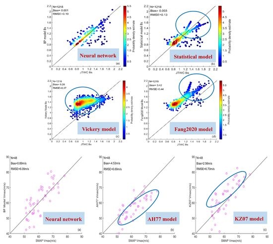
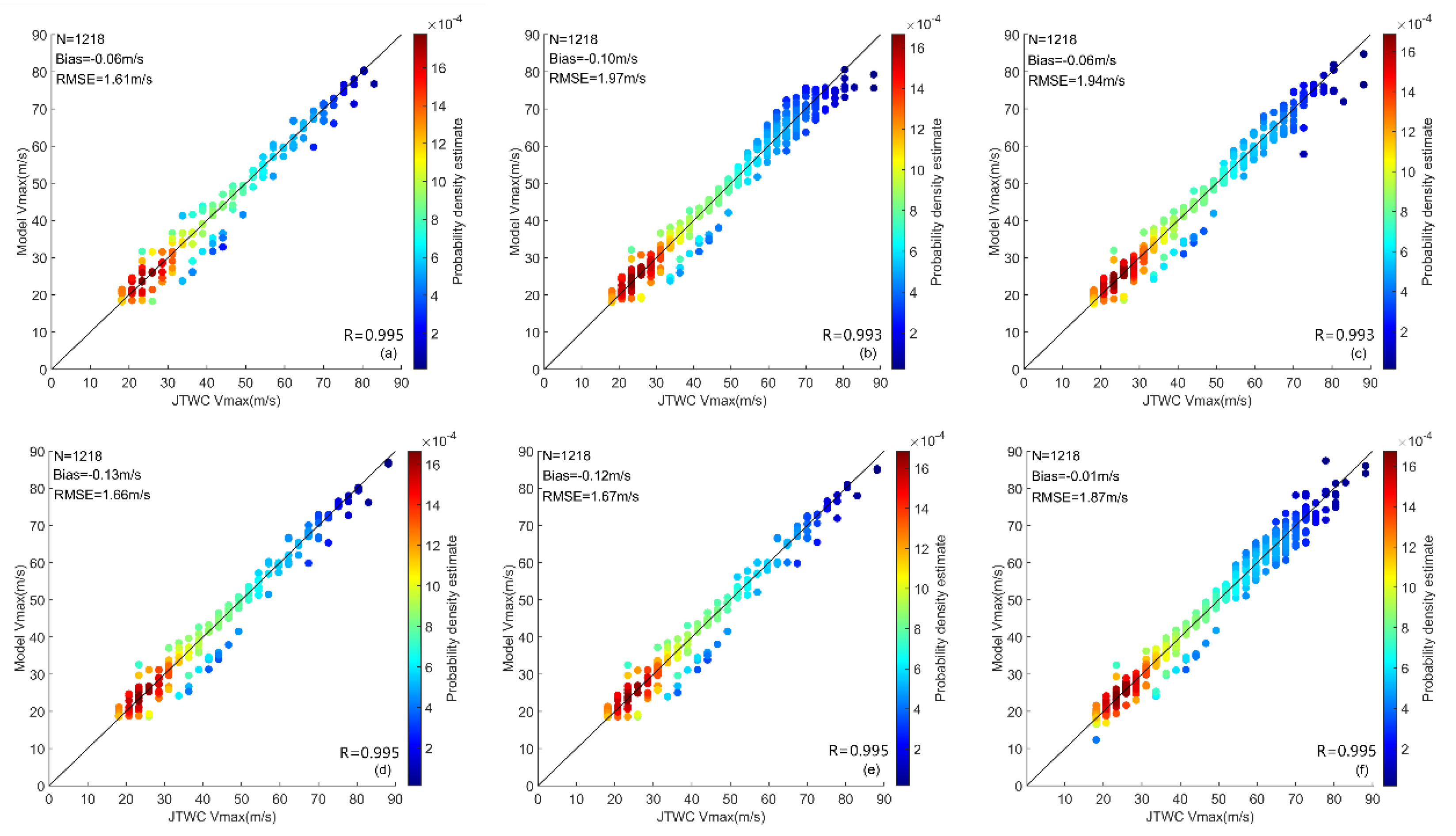
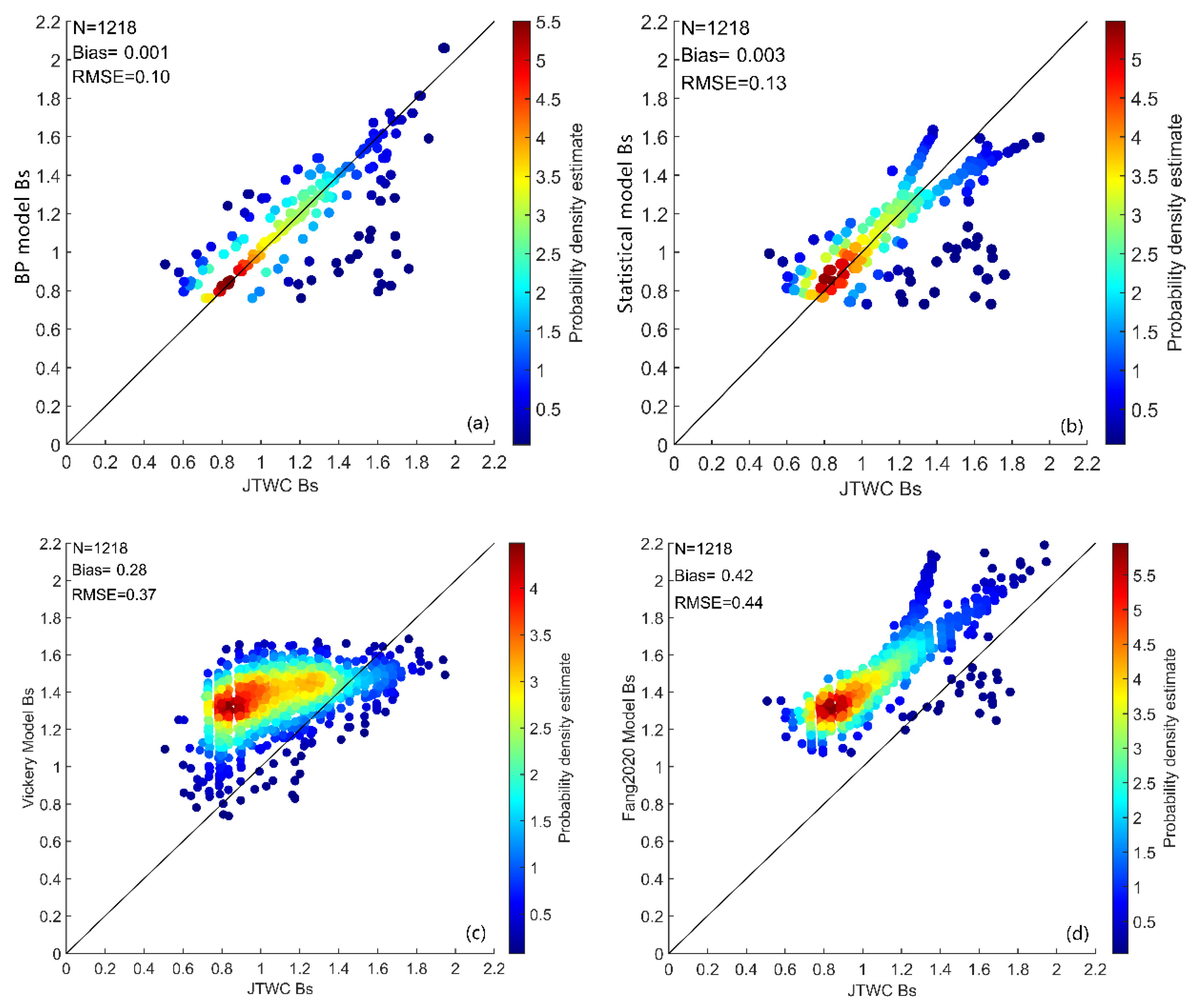
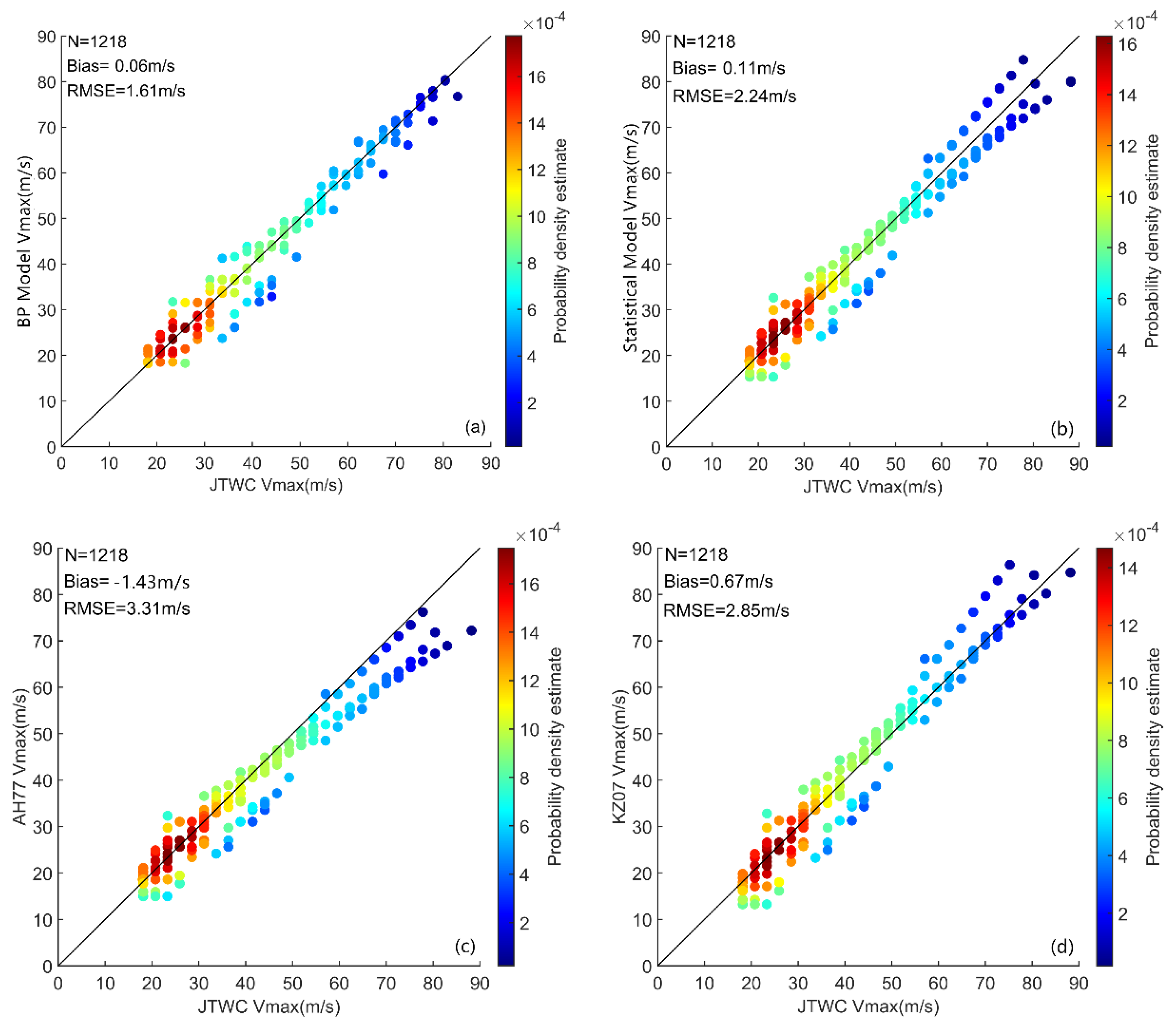
• Comparing the simulation results of the network constructed by different input schemes for the testing data reveals that the neural network only considers inputting TC center pressure difference has the best performance. The deviation and RMSE of $B_s$ are only −0.001 and 0.10. The MWS of TCs calculated by the constructed $B_s$ neural network combined with the wind pressure model is compared with the MWS of JTWC. The result also shows that the neural network that only considers TC center pressure difference performs best and the deviation and RMSE of MWS are only 0.06 and 1.61 m/s.
• The results of the statistical models established in this study, also show that the TC central pressure difference is the most important factor to $B_s$ and the introduction of other variables does not significantly improve the model results. When the $B_s$ value is greater than 1.2, the simulation results of these statistical models exhibit significant underestimation or overestimation. The Fang2020 model also represents a similar phenomenon when simulating $B_s$. However, the $B_s$ neural network in this study can significantly improve the underestimation and overestimation, indicating that the BP neural network can capture the nonlinear distribution of the $B_s$ values that cannot be described by traditional statistical methods and obtain a more accurate value of the $B_s$ parameter.
• To study the details of the model in different typhoon cases, we divide the testing data into super typhoon group and nonsuper typhoon group according to typhoon intensity. For the super typhoon group, the MWS simulated by the two existing wind pressure models, the AH77 model and the KZ07 model is underestimated and overestimated. The deviations are −4.76 and 2.53 m/s, whereas the deviation of $B_s$ neural network is appropriate (0.14 m/s). For the nonsuper typhoon group, the performance gap of the three models is not so remarkable. It shows that our $B_s$ neural network has more advantages in simulating the MWS of super typhoons.
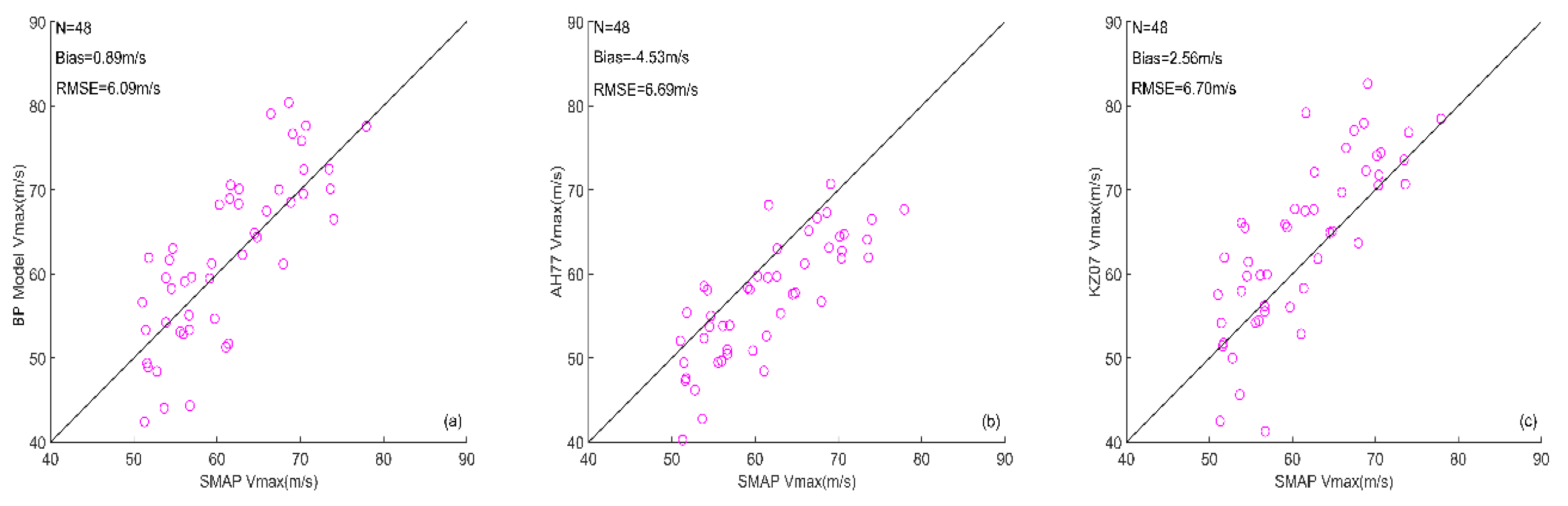
• The MWS of super typhoons observed by the spaceborne microwave radiometer SMAP is also used to verify the network in detail. The experimental results show that the simulated MWS of the AH77 model is significantly underestimated, with a deviation of −4.53 m/s and the simulated MWS of the KZ07 model is overestimated, with a deviation is 2.56 m/s. Our $B_s$ neural network, whose deviation is only 0.89 m/s, also improves the underestimation and overestimation phenomena.

The $B_s$ neural network established in this study only needs to input the TC central pressure difference to simulate the sea surface wind field Holland B parameter $B_s$ accurately. After the wind pressure model has been combined, the $B_s$ neural network can simulate the MWS of super typhoons better than the existing wind pressure models. However, given that the data used in this study exclude landing TCs, the model is mainly suitable for open water. Building a more accurate $B_s$ model for coastal areas is one of our future considerations.

References

1. Harper, B.A. Tropical Cyclone Parameter Estimation in the Australian Region: Wind–Pressure Relationships and Related Issues for Engineering Planning and Design—A Discussion Paper; Systems Engineering Australia Party Ltd.: Newstead, Australia, 2002; SEA Rep. J0106-PR003E; p. 83. [Google Scholar]
2. Atkinson, G.D.; Holliday, C.R. Tropical Cyclone Minimum Sea Level Pressure/Maximum Sustained Wind Relationship for the Western North Pacific. Mon. Weather. Rev. 1977, 105, 421–427. [Google Scholar] [CrossRef] [Green Version]
3. Knaff, J.A.; Zehr, R.M. Reexamination of Tropical Cyclone Wind–Pressure Relationships. Weather. Forecast. 2007, 22, 71–88. [Google Scholar] [CrossRef]
4. Schloemer, R.W. Analysis and Synthesis of Hurricane Wind Patterns over Lake Okeechobee, Florida; U.S. Department of Commerce, Weather Bureau: Washington, DC, USA, 1954. [Google Scholar]
5. Holland, G.J. An Analytic Model of the Wind and Pressure Profiles in Hurricanes. Mon. Weather. Rev. 1980, 108, 1212–1218. [Google Scholar] [CrossRef]
6. Love, G.; Murphy, K. The Operational Analysis of Tropical Cyclone Wind Fields in the Australian Northern Region. North. Territ. Reg. Res. Papers 1984, 85, 44–51. [Google Scholar]
7. Hubbert, G.D.; Holland, G.J.; Leslie, L.M.; Manton, M.J. A Real-Time System for Forecasting Tropical Cyclone Storm Surges. Weather. Forecast. 1991, 6, 86–97. [Google Scholar] [CrossRef] [Green Version]
8. Harper, B.A.; Holland, G.J. An updated parametric model of the tropical cyclone. In Proceedings of the 23rd Conference Hurricanes and Tropical Meteorology, Dallas, TX, USA, 10–15 January 1999. [Google Scholar]
9. Vickery, P.J.; Skerlj, P.F.; Steckley, A.C.; Twisdale, L.A. Hurricane Wind Field Model for Use in Hurricane Simulations. J. Struct. Eng. 2000, 126, 1203–1221. [Google Scholar] [CrossRef]
10. Willoughby, H.; Rahn, M. Parametric representation of the primary hurricane vortex. Part I: Observations and evalua-tion of the Holland (1980) model. Mon. Weather Rev. 2004, 132, 3033–3048. [Google Scholar] [CrossRef]
11. Jakobsen, F.; Madsen, H. Comparison and further development of parametric tropical cyclone models for storm surge modelling. J. Wind. Eng. Ind. Aerodyn. 2004, 92, 375–391. [Google Scholar] [CrossRef]
12. Powell, M.; Soukup, G.; Cocke, S. State of florida hurricane loss projection model: Atmospheric science component. J. Wind Eng. Ind. Aerodyn. 2005, 93, 651–674. [Google Scholar] [CrossRef] [Green Version]
13. Vickery, P.J.; Dhiraj, W. Statistical models of Holland pressure profile parameter and radius to maximum winds of hurricanes from flight-level pressure and H*Wind data. J. Appl. Meteorol. Climatol. 2008, 47, 2497–2517. [Google Scholar] [CrossRef]
14. Holland, G. A Revised Hurricane Pressure–Wind Model. Mon. Weather. Rev. 2008, 136, 3432–3445. [Google Scholar] [CrossRef] [Green Version]
15. Xiao, Y.; Duan, Z.; Ou, J.; Chang, L.; Li, Q. Typhoon wind hazard analysis for southeast China coastal regions. Struct. Saf. 2011, 33, 286–295. [Google Scholar] [CrossRef]
16. Lin, W.; Fang, W.H. Study on regional characteristics of Holland B parameter in typhoon wind field model for Northwest Pacific. Trop. Geogr. 2013, 33, 124–132. [Google Scholar]
17. Li, S.H.; Hong, H.P. Use of historical best track data to estimate typhoon wind hazard at selected sites in China. Nat. Hazards 2014, 76, 1395–1414. [Google Scholar] [CrossRef]
18. Zhao, L.; Lu, A.; Zhu, L.; Cao, S.; Ge, Y. Radial pressure profile of typhoon field near ground surface observed by distrib-uted meteorologic stations. J. Wind Eng. Ind. Aerodyn. 2013, 122, 105–112. [Google Scholar] [CrossRef]
19. Fang, G.; Zhao, L.; Song, L.; Liang, X.; Zhu, L.; Cao, S. Reconstruction of radial parametric pressure field near ground sur-face of landing typhoons in northwest pacific ocean. J. Wind Eng. Ind. Aerodyn. 2018, 183, 223–234. [Google Scholar] [CrossRef]
20. Fang, P.; Ye, G.; Yu, H. A parametric wind field model and its application in simulating historical typhoons in the western North Pacific Ocean. J. Wind. Eng. Ind. Aerodyn. 2020, 199, 104131. [Google Scholar] [CrossRef]
21. Meissner, T.; Ricciardulli, L.; Wentz, F.J. Capability of the SMAP Mission to Measure Ocean Surface Winds in Storms. Bull. Am. Meteorol. Soc. 2017, 98, 1660–1677. [Google Scholar] [CrossRef]
22. Yueh, S.H.; Fore, A.G.; Tang, W.; Hayashi, A.; Stiles, B.; Reul, N. SMAP L-Band Passive Microwave Observa-tions of Ocean Surface Wind During Severe Storms. IEEE Trans. Geosci. Remote 2016, 54, 7339–7350. [Google Scholar] [CrossRef]
23. Fore, A.G.; Yueh, S.H.; Stiles, B.W.; Tang, W.; Hayashi, A.K. SMAP Radiometer-Only Tropical Cyclone Intensity and Size Validation. IEEE Geosci. Remote Sens. Lett. 2018, 15, 1480–1484. [Google Scholar] [CrossRef]
24. Sun, Z.; Zhang, B.; Zhang, J.A.; Perrie, W. Examination of Surface Wind Asymmetry in Tropical Cyclones over the Northwest Pacific Ocean Using SMAP Observations. Remote Sens. 2019, 11, 2604. [Google Scholar] [CrossRef] [Green Version]
25. Olfateh, M.; Callaghan, D.P.; Nielsen, P.; Baldock, T.E. Tropical cyclone wind field asymmetry-Development and evaluation of a new parametric model. J. Geophys. Res. Ocean. 2017, 122, 458–469. [Google Scholar] [CrossRef]
26. Kang, N.-Y.; Elsner, J.B. Consensus on Climate Trends in Western North Pacific Tropical Cyclones. J. Clim. 2012, 25, 7564–7573. [Google Scholar] [CrossRef] [Green Version]
Figure 1. Influence of adjusting the Holland B parameter on the radial profiles of (a) sea surface pressure and (b) gradient wind speed. The values of ambient pressure ( P n ), central pressure ( P c ) and the RMW of the TC are marked on the figure and the abscissa indicates the radial distance from the observation point to the center of the TC. Curves of different colors represent Holland B parameters of different values.
Remotesensing 13 02653 g001
Figure 2. Geographic distribution density map of the TC center location that has passed the quality control standards (for the training data). The darker the color, the more the number of TCs. The red hollow circles represent the distribution of the TC center location (for the testing data). The horizontal and vertical coordinates stand for longitude and latitude.
Remotesensing 13 02653 g002
Figure 3. Histogram of key parameters of TCs from the JTWC best-track dataset in the training data for (a) TC intensity ( V m a x ), (b) TC central pressure difference ( Δ P =   P n P c ), (c) RMW, (d) latitude ( ), (e) TC moving speed ( V s t o r m ) and (f) TC intensity change rate ( p c / t ).
Remotesensing 13 02653 g003
Figure 4. Central pressure ( P c ) versus B s parameter for the (a) training data and (b) testing data. The color bar represents the probability density estimate of each point.
Remotesensing 13 02653 g004
Figure 5. Topology of the BP neural network.
Remotesensing 13 02653 g005
Figure 6. Holland B s parameter versus (a) TC central pressure difference   ( Δ P =   P n P c ) , (b) RMW, (c) latitude of the TC center   ( ), (d) TC translation speed ( V s t o r m ) and (e) TC intensity change rate ( p c / t ) for the training data. The formula of the best fitting line of each independent variable and the square of the correlation coefficient ( R 2 ) are marked at the top of each panel. The color bar represents the probability density estimate of each point.
Remotesensing 13 02653 g006
Figure 7. Comparison results between the B s values simulated by (a) Network-1, (b) Network-2, (c) Network-3, (d) Network-4, (e) Network-5, (f) Network-6 and the B s values calculated from JTWC in the testing data. The abscissa stands for the B s values calculated from JTWC and the ordinate is the simulated B s values. The number of samples (N), deviation (Bias), RMSE and correlation coefficient (R) of each comparison result are marked at the top and bottom of each panel. The color bar represents the probability density estimate of each point.
Remotesensing 13 02653 g007
Figure 8. Comparison results between the MWS simulated by (a) Network-1, (b) Network-2, (c) Network-3, (d) Network-4, (e) Network-5, (f) Network-6 combined with Equation (8) and that of JTWC in the testing data. The abscissa stands for the MWS from JTWC and the ordinate is the simulated MWS. The number of samples (N), deviation (Bias), RMSE and correlation coefficient (R) of each comparison result are marked at the top and bottom of each panel. The color bar represents the probability density estimate of each point.
Remotesensing 13 02653 g008
Figure 9. RMW versus TC central pressure difference ( Δ P =   P n P c ) in the training data. Red bars stand for mean and mean +/− STD of Δ P within each 10 km bin in RMW of JTWC.
Remotesensing 13 02653 g009
Figure 10. Comparison results between the B s values simulated by (a) expression-1, (b) expression -2, (c) expression -3, (d) expression -4, (e) expression-5, (f) expression-6 in Table 4 and the B s values calculated from JTWC in the testing data. The abscissa stands for the B s values calculated from JTWC and the ordinate is the simulated B s values. The number of samples (N), deviation (Bias), RMSE and correlation coefficient (R) of each comparison result are marked at the top and bottom of each panel. The color bar represents the probability density estimate of each point.
Remotesensing 13 02653 g010
Figure 11. Comparison results between the B s values calculated from JTWC in the testing data and the B s values simulated by (a) the BP neural network (Network-1 shown in Figure 7a and Figure 11a), (b) the statistical model ((1) in Table 4), (c) the Vickery model ((8) in Table 1) and (d) the Fang2020 model ((13) in Table 1). The abscissa stands for the B s values calculated from JTWC and the ordinate is the simulated B s values. The number of samples (N), deviation (Bias) and RMSE of each comparison result are marked at the top of each panel. The color bar represents the probability density estimate of each point.
Remotesensing 13 02653 g011
Figure 12. Comparison results between the MWS of JTWC in the testing data and the MWS simulated by (a) the BP neural network (Network-1) combined with Equation (8), (b) the statistical model ((1) in Table 4) combined with Equation (8), (c) the AH77 model (Equation (2)) and (d) the KZ07 model (Equation (4)). The abscissa stands for the MWS from JTWC and the ordinate is the simulated MWS. The number of samples (N), deviation (Bias) and RMSE of each comparison result are marked at the top of each panel. The color bar represents the probability density estimate of each point.
Remotesensing 13 02653 g012
Figure 13. Comparison results between the MWS of JTWC in the testing data and the MWS simulated by (a) the BP neural network (Network-1), (b) the AH77 model (Equation (2)), (c) the KZ07 model (Equation (4)) combined with Equation (8), (d) the BP neural network (Network-1), (e) the AH77 model (Equation (2)) and (f) the KZ07 model (Equation (4)) combined with Equation (8). (ac) is for MWS greater than 51 m/s and (df) is for MWS less than 50.9 m/s. The abscissa stands for the MWS from JTWC and the ordinate is the simulated MWS. The number of samples (N), deviation (Bias) and RMSE of each comparison result are marked at the top of each panel. The color bar represents the probability density estimate of each point.
Remotesensing 13 02653 g013
Figure 14. Comparison results between the MWS of SMAP and the MWS simulated by (a) the BP neural network (Network-1) combined with Equation (8), (b) the AH77 model (Equation (2)) and (c) the KZ07 model (Equation (4)). The abscissa stands for the MWS from SMAP and the ordinate is the simulated MWS. The number of samples (N), deviation (Bias) and RMSE of each comparison result are marked at the top of each panel.
Remotesensing 13 02653 g014