Mapping Water Infiltration Rate Using Ground and UAV Hyperspectral Data: A Case Study of Alento, Italy

Abstract

Water infiltration rate (WIR) into the soil profile was investigated through a comprehensive study harnessing spectral information of the soil surface. As soil spectroscopy provides invaluable information on soil attributes, and as WIR is a soil surface-dependent property, field spectroscopy may model WIR better than traditional laboratory spectral measurements. This is because sampling for the latter disrupts the soil-surface status. A field soil spectral library (FSSL), consisting of 114 samples with different textures from six different sites over the Mediterranean basin, combined with traditional laboratory spectral measurements, was created. Next, partial least squares regression analysis was conducted on the spectral and WIR data in different soil texture groups, showing better performance of the field spectral observations compared to traditional laboratory spectroscopy. Moreover, several quantitative spectral properties were lost due to the sampling procedure, and separating the samples according to texture gave higher accuracies. Although the visible near-infrared–shortwave infrared (VNIR–SWIR) spectral region provided better accuracy, we resampled the spectral data to the resolution of a Cubert hyperspectral sensor (VNIR). This hyperspectral sensor was then assembled on an unmanned aerial vehicle (UAV) to apply one selected spectral-based model to the UAV data and map the WIR in a semi-vegetated area within the Alento catchment, Italy. Comprehensive spectral and WIR ground-truth measurements were carried out simultaneously with the UAV–Cubert sensor flight. The results were satisfactorily validated on the ground using field samples, followed by a spatial uncertainty analysis, concluding that the UAV with hyperspectral remote sensing can be used to map soil surface-related soil properties.

1. Introduction

The water infiltration rate (WIR) into the soil profile is a very important hydrological property that controls runoff, leaching, soil erosion, and water availability for both plants and ground water [1]. It is therefore assumed that assessing and controlling the WIR in a spatial domain is critical for combating desertification processes in the current era of global warming [2].

To achieve this, rapid and effective monitoring methodologies are needed to measure WIR, which is affected by several factors. These factors can be divided into local and regional parameters. The regional parameters are the topography [3] (mainly the slope that governs runoff) and the landscape characteristics (mainly land coverage) [4,5,6,7,8,9]; the local parameters are the soil profile characteristics such as soil moisture [10], organic matter (OM) content [11], soil mineralogy [12], soil texture [12,13], soil sealing [14,15], soil structure [16] and the arrangement of diagnostic layers of the soil profile. The soil surface is defined as the interface between the atmosphere and the pedosphere, and hence is the most critical layer where free water meets the soil body. Whereas clayey soils (or layer) with expanding 2:1 phyllosillicate minerals (also known as “swelling soils”) may decrease WIR values, sandy soils (or layer) tend to increase them [12,13,14,15,17]. High WIR values are generally considered a positive soil characteristic, and the negative effects of low WIR are of great concern. Within the local parameters, low WIR can be due to a physical soil crust (e.g., fine structure of the soil surface) [14,15,17], biogenic crust (e.g., cyanobacteria) [18] or chemical crust (e.g., salinity) [14]. The positive effects of high WIR are due to OM [11,19], carbonates [20], and other binding agents, such as those contributed to by microorganisms that stabilize soil aggregation and thereby increase the WIR process [21]. Another positive factor for WIR is plant litter or vegetation cover [22], which tends to reduce rain drop energy on the soil surface and, accordingly, minimizes the formation of a physical crust [23]. As the soil surface is affected by climatic factors (e.g. rain drop energy, sun heating and dust accumulation), biological factors (e.g., cyanobacteria) [18], and agricultural management practices (packing or plowing), monitoring the WIR at the local surface level is important for saving water, preventing erosion, and improving crops’ yields [1,2,3,4,5,6,7,8,9,10,11,12,13,14,15,16,17,18,19,20,21,22,23].

The instrumentation for measuring WIR in the field varies from complicated, such as field rain simulators [24], to simple, such as point infiltrometers [25], the latter being easier to transport and operate. Nevertheless, both methods are time consuming and costly, involving point orientation, and requiring qualified and highly skilled personnel, especially when covering large areas for mapping purposes. Soil spectroscopy across the 400–2500 nm spectral range is a precise way of simplifying the soil system’s complexity as it enables the estimation of many soil attributes in a rapid and convenient way [26]. Today, there are many soil spectral libraries (SSLs) available worldwide with spectral- and laboratory-evaluated properties such as texture, OM, calcium carbonates, cation-exchange capacity, and pH among others [27,28,29,30]. These SSLs can be used to develop spectral-based models, which can then be exploited to predict soil properties without the need for expensive and time-consuming wet laboratory analyses. The added value of soil spectroscopy lies in its rapid measurements and rapid provision of information on soil attributes and, especially, its possible execution using remote sensing (RS) means—both point and spectral imaging sensors. This capability enables a spatial illustration of the soil properties available in the SSLs over bare soils. The ability to derive WIR spectrally was demonstrated by Ben-Dor et al. [31] and later by Goldshleger et al. [32]. These authors collected soils that were subjected to different and controlled rain energies using a rain simulator in the laboratory. Then, these samples were subjected to laboratory spectral measurements to generate a spectral-based model to predict WIR. In Ben-Dor et al. [31], the spectral-based model was run with airborne hyperspectral remote sensing (HRS) data to quantitatively map the WIR in a selected field. Nevertheless, in those studies [31,32], the soil samples still had to be collected and packed in boxes for the laboratory spectral measurements after applying artificial rain. This sampling methodology is problematic because the soil surface (and therefore the crust) is disturbed by the field sampling as well as by the packing. Accordingly, in the reported works [31,32], the surface condition of the soil was not reproduced and a WIR map could not be adequately obtained.

As spectral analyses across the 400–2500 nm spectral range appear to be sensitive to WIR [31,32], it is postulated that they can provide precise measurements and a good representation of the real soil conditions in the field. This direction is doubly important: First, it will enable accurate and rapid field WIR measurements using point spectrometers and, second, it will enable RS practices to better represent the field WIR status spatially from afar. We assume that traditional SSLs, which are generated in the laboratory, will have some uncertainties regarding real field conditions. Accordingly, a new strategy that relies on spectral measurements in the field under natural conditions must be adopted for correct spectral-based modeling of soil surface-dependent properties. Our aim in this paper was therefore to develop this field-based spectral approach using a novel apparatus [33] to measure soil reflectance in the field with laboratory quality and to examine it over a well-documented agricultural field [34] in Alento, Italy. We generated a comprehensive field-based SSL (FSSL) of undisturbed soil samples, followed by reliable WIR measurements in the field. The same FSSL samples were spectrally measured in the laboratory to evaluate the gap between laboratory and spectral observations. We also examined the performance of a spectral-based model generated from the FSSL to predict the WIR on a raster dataset acquired by a hyperspectral camera onboard an unmanned aerial vehicle (UAV). The predictions were further examined with field observations of the measured WIR and spatial uncertainty analyses of hot and cold spots [35,36].

2. Materials and Methods

2.1. Study Sites

2.1.1. The UAV Campaign Study Site: Alento, Italy

For this study, we selected an agricultural field located in the Alento River catchment, in southern Italy. The Alento catchment has long been a critical observatory for monitoring climate change, hydrological processes, anthropogenic disturbances, drought conditions, etc. [34,37,38]. The Alento River catchment is located in the Campania region (Salerno Province, Italy). Alento has a Mediterranean climate (Csa) [39] and is characterized by hills and mountains on limestone covered by volcanic ash, and alluvial and coastal plains [34]. Three soil types are common in the Alento river catchment: Cambisols, Leptosols, and Luvisols [40], but the samples that were collected from the examined study site of the Alento basin were all classified as Leptosols (WRB-FAO classification), where the soil is clayey–calcareous [34]. The center of the selected site was located at 40°21′53.68″N, 15°11′1.42″E.

2.1.2. Mediterranean Sites for Generating the FSSL

A comprehensive FSSL with 114 soil samples was created to generate spectral-based models to map the WIR in Alento and to study the gap between laboratory and field spectral observations. To build the FSSL, we selected six areas (including Alento) across three countries along the Mediterranean basin: Israel, Italy, and Greece. The samples were collected from the following fields:

I.

Alento, Italy (21 samples): The area described above.

II.

Kibbutz Sde Yoav, Israel (30 samples): Kibbutz Sde Yoav is an agricultural settlement located in southcentral Israel, between the cities of Ashkelon, Kiryat Gat, and Kiryat Malakhi. The soil type in the study area is alluvial [41] (Fluvisol according to the WRB-FAO general classes). According to an updated version of the Köppen climate classification [39], the climate is hot-semiarid (Bsh). The center of the study site is located at 31°38′35″N, 34°40′15″E.

III.

Afeka, Tel Aviv, Israel (18 samples): Afeka is a residential neighborhood located in north Tel Aviv. The soil type in the study area is brown-red sandy soil [42] (Ferralsol according to the WRB-FAO reference soil groups), and the climate is hot-summer Mediterranean (Csa). The samples at this study site were collected around the coordinates 32°7′9.16″N, 34°48′14.84″E.

IV.

Central Macedonia, Greece (45 samples from three different fields): Three different agricultural fields were selected in this region. The climate is hot-summer Mediterranean (Csa) [39]. According to the WRB-FAO reference soil groups, the soil type in the first field (40°37′32.03″N, 21°34′1.23″E) is classified as Fluvisol. The second (40°39′55.31″N, 21°36′20.49″E) and third (40°40′11.46″N, 21°37′56.67″E) field soils are classified as Cambisol [43].

Figure 1a illustrates the Mediterranean basin area and the locations at the centers of the selected sites from which samples were collected. The locations of the selected agricultural fields in Greece are zoomed in on in Figure 1b.

2.2. Field and Laboratory Data Acquisition

In the selected fields (including Alento), the in-situ undisturbed soil surface was spectrally measured at different points, simultaneously with WIR measurements at each point. This process was followed by soil (disturbed) sampling from the top 5 cm of the measured point for further laboratory analyses. The samples were dried and gently ground in the laboratory to pass through a 2 mm sieve. All of the field measurements were performed during the Mediterranean summer, where the soil was air-dried with no vegetation or litter over the measurement spots. The Alento field measurements were taken on 13 June 2019 simultaneously with an UAV overpass (see Section 2.3).

The spectral measurements were taken with an ASD FieldSpec^® spectrometer (Analytical Spectral Devices, model FSP 350-2500P). This device measures the reflected light in 2151 bands within the 350–2500 nm spectral range and consists of three discrete detectors: visible near-infrared (VNIR; 350–1000 nm), shortwave infrared 1 (SWIR1) (1001–1800 nm), and SWIR2 (1801–2500 nm). In the VNIR detector, the full-width-half-maximum (FWHM) is approximately 3 nm, and in both the SWIR1 and SWIR2 detectors, the FWHM is approximately 10 nm. The spectrometer was configured to take an average of 30 spectral readings for each spectral measurement performed in the field and in the laboratory. Spectral reflectance in the field and laboratory was calculated relative to a Halon white reference panel (Spectralon, Labsphere Inc., North Sutton, NH, USA). The laboratory spectral measurements were conducted following the internal soil standard (ISS) protocol suggested by Ben Dor et al. [44] with LB soil standards.

In the field, the ASD was hooked up to a SoilPRO^® assembly [33] that was developed at Tel Aviv University to measure the soil surface reflectance while preserving the field condition (undisturbed). The system provides laboratory-quality spectral readings in the field by eliminating atmospheric attenuation and variations in solar illumination and by preserving a constant measurement geometry. The SoilPRO is furnished with a halogen tungsten lamp at a fixed geometry that covers around 200 cm² [33]. The spectral readings were calculated against a white reference Halon panel that covered the entire field of view of the fore optic. For the spectral measurements, three repetitions were performed at each site and then averaged for a representative spectrum.

The field measurements of WIR were performed using a minidisk infiltrometer (METER Group Inc., Pullman, WA, USA) [25] and the following protocol: a negative pressure head of 2 cm was applied at the soil surface, and the volume of the infiltrated water over time was recorded every 30 s for at least 5 min. According to the minidisk infiltrometer user manual, to calculate the WIR values, the texture of the soil samples needs to be estimated. Texture classification was performed following the field method of Thien [45] to determine the most representative texture of every measurement point. Once the texture of every sample was classified, the most representative classification per field was assigned to every sample according to the field’s texture class.

Table 1. Texture classes based on the assigned texture classification of the studied sites.

Field	Country	No. of Samples	Classification	Texture Group
Sde Yoav	Israel	30	Clay Loam	Clayey (heavy)
Afeka	Israel	18	Sandy Clay Loam	Clayey (heavy)
Alento	Italy	21	Loam	Clayey (heavy)
C. Macedonia 1	Greece	16	Sand	Sandy (light)
C. Macedonia 2	Greece	15	Sandy Loam	Sandy (light)
C. Macedonia 3	Greece	14	Sandy Loam	Sandy (light)

illustrates the texture assigned to each field, which varied from sand to loam clayey soils.

As the WIR is considerably affected by the soil texture, the samples were grouped into two textural categories to examine whether fine-tuning according to their texture would provide better accuracy. Accordingly, three groups were evaluated as follows:

I.

The whole dataset: samples collected from all sites (114 samples).

II.

The “sandy” dataset: samples from Afeka (Tel Aviv), Israel and from the three fields in Central Macedonia, Greece (58 samples).

III.

The “clayey” dataset: samples from Sde Yoav, Israel and Alento, Italy (46 samples).

Thus, two groups of soil were created: The first was characterized by a high sand content (>50%) and termed the “sandy” group (light soils), and the second was characterized by a low sand content (<50%) and termed the “clayey“ group (heavy soils) (see Table 1). This was based on the USDA texture triangle where the soil classifications were obtained by an expert in the field using Thien’s [45] qualitative methods. Those samples that had negative WIR were equalized to zero for display on the maps (in Section 3) because we assumed that their real WIR value was extremely low. This problem has been previously reported in the literature and has been related to hydrophobicity, soil moisture, and/or measurement errors [10]. Before each field measurement, we spoke with local farmers to ensure that the fields had not been irrigated during the previous 14 days.

2.3. The UAV Data Acquisition

During the field data acquisition over the Alento site, we conducted an UAV mission. For the UAV campaign, we used the Cubert UHD-185^® camera, which is a hyperspectral snapshot sensor installed onboard a CarbonCore Cortex X8 UAV platform with a Pixhawk 2 Cube flight controller. The Cubert UHD-185 sensor measures the reflected light across the 450–950 nm (VNIR) spectral range with 125 spectral bands and a dynamic range of 12 bits collected within a 4 nm sampling interval. The images were acquired on a sunny, clear-sky day (13 June 2019) between 09:57 a.m. and 10:30 a.m. (Central European Summer Time) in an approximately 7 ha agricultural field close to Montiforte Cilento located in the Alento catchment, Italy (exact location is given in Section 2.1.1). The UAV data were acquired from a relative flight altitude of 138 m above ground level in terrain-following mode, providing a unified pixel size of 4.6 cm in all images. To generate a mosaic image, we used 468 images for which we applied 80% forward overlap and 65% sidelap during flight. For orthorectification of the image block, we used a HiPer V (Topcon) GNSS receiver to measure six high-accuracy ground control points and three checkpoints, which presented root mean square errors (RMSEs) of 2.0 cm and 7.3 cm, respectively, after the geometric transformation. The locations of the field samples collected in the study area were also measured using the HiPer V (Topcon) GNSS receiver. The digital numbers (DN) of the Cubert UHD-185 sensor were calibrated to reflectance using the Halon white reference, measured before take-off. To validate the UAV reflectance calibration, we used one white panel and four black agricultural nets with increasing densities folded over four white panels (Figure 2). All of the white panels were identical. The panels were measured with the SoilPRO assembly to form a set of validation targets for field and UAV spectral measurements.

2.4. Data Analysis

As the laboratory and field spectral data were resampled to the Cubert spectral configuration, two spectral resolutions were examined for the spectral modeling of WIR. For the spectral-based models that were generated before resampling the spectral data to the Cubert resolution, we used the original 450–2400 nm (VNIR–SWIR region) spectral range (ASD). Then, for the spectral-based models with the resampled data, we used the 482–902 nm (VNIR region) spectral range and the FWHM of the Cubert. In addition, the soil samples were grouped according to their assigned texture to examine whether fine-tuning based on texture would provide better accuracy and to select a set of samples that could better represent the texture classification of the study area.

Before generating the spectral-based models, we observed the average field and laboratory spectra for every field (using all points) to look for any important differences. In addition, to determine what spectral information was distorted after the sampling procedures, we calculated the average spectral ratio between the field and laboratory spectra. To recognize what soil properties with spectral assignments might be distorted by the sampling procedures, we used the publications of Viscarra Rossel and Bahrens (2010) [46] and Ben-Dor [26].

For the laboratory and field spectral-based models that were generated using the ASD and the Cubert spectral configurations, the data were randomly split, retaining the same samples (in both the laboratory and the field) to perform the calibration and validation steps under the same conditions; 20% of the samples were selected for validation, and 80% for calibration. To model the WIR, we selected partial least squares regression (PLSR) [47] because it is an effective and well-known method in chemometrics and spectral-based analyses [26,47] and has been successfully used to estimate normally and non-normally distributed parameters [48,49,50,51]. Moreover, Zhao et al. [52] recently showed that PLSR can provide higher accuracies than other machine learning algorithms (Cubist, random forests, and support vector machines). In the present manuscript, the PLSR models were developed using the scikit-learn package of Python 3.7 [53].

The performance of the spectral-based models was evaluated using R², RMSE, and the ratio of performance to interquartile distance (RPIQ) [54], where low RMSE and high R² and RPIQ values indicate good performance. The equations describing the employed statistics are as follows:

$$R^2=1-\frac{{\sum }_{i=1}^n{\left(Y_i-{\widehat{Y}}_i\right)}^2}{{\sum }_{i=1}^n{\left(Y_i-{\overline{Y}}_i\right)}^2}$$

(1)

$$RMSE=\sqrt{{\displaystyle \sum }_{I=1}^n\frac{{\left({\widehat{Y}}_i-Y_i\right)}^2}{n}}$$

(2)

$$RPIQ=IQ/RMSE$$

(3)

where Ŷ is the predicted value, Ȳ is the mean of observed values, Y is the observed value, n is the number of data points, and IQ is the interquartile distance of the measured values.

The following preprocessing scenarios were examined: reflectance with no preprocessing, Savitzky–Golay (SG) first derivative of reflectance, continuum removal of reflectance, and SG first derivative of absorbance. To enable comparisons under the same processing conditions between the laboratory- and field-based models, we maintained the same spectral preprocessing and the same number of PLSR components in every comparison. The spectral preprocessing and the number of components for each scenario were selected by examining the lowest RMSE obtained in the validation phase of the field spectral-based models, assuming that this dataset better represents the field conditions for the WIR estimation.

Once the best field spectral-based model was obtained, the gap between the field and laboratory spectral observations was analyzed using the beta coefficients generated by the PLSR models. The beta coefficients summarize the most important spectral features for the estimation of WIR in each spectral-based model [47]. To analyze the beta coefficients, we followed the publications of Viscarra Rossel and Bahrens [46] and Ben-Dor [26], who summarized several recognizable soil properties according to their indicative wavelengths. The beta coefficients of the original ASD spectral resolution were smoothed to better emphasize the most indicative wavelengths. This procedure was not necessary with the Cubert UHD-185 spectral resolution because the spectral sampling interval of the Cubert UHD-185 is larger than that of the ASD (4 and 1 nm, respectively). This examination can indicate what quantitative spectral information is lost with the resampling procedures, and the gap between field and laboratory spectral observations can be further analyzed.

2.5. Spectral Similarity Analysis

To compare the UAV output with the field spectral observations, we carried out a spectral similarity analysis using the white panels that were covered with different densities of black agricultural net (validation targets). To further validate the UAV observations, this similarity analysis was repeated for five soil samples that were collected at the Alento study site and were not part of the calibration phase of the spectral-based model, which was executed in the UAV hyperspectral image. To conduct the spectral similarity analysis, we used a modified version of the average sum of deviations squared (ASDS) index [55] termed as M–ASDS, using the following equations:

$$M–ASDS=\frac{{{\displaystyle \sum }}_{i=1}^n{\left(R{r}_n-1\right)}^2}{n}$$

(4)

where n is the number of wavelengths used, and Rr_n was calculated as:

$$R{r}_n=\frac{\left({Rt}_n+1\right)}{({Rtr}_n+1)}$$

(5)

where Rt_n is the examined reflectance spectrum (i.e., Cubert), and Rtr_n is the reference spectrum (i.e., field) of the same target. Rr_n represents the ratio between the examined and reference spectra but with an added unit (to both the numerator and the denominator) to correct the bias caused by dark targets. If this is not carried out, targets with very low reflectance may increase the ASDS index, although they could have minimal spectral variations relative to the examined spectra.

2.6. Spatial Analysis

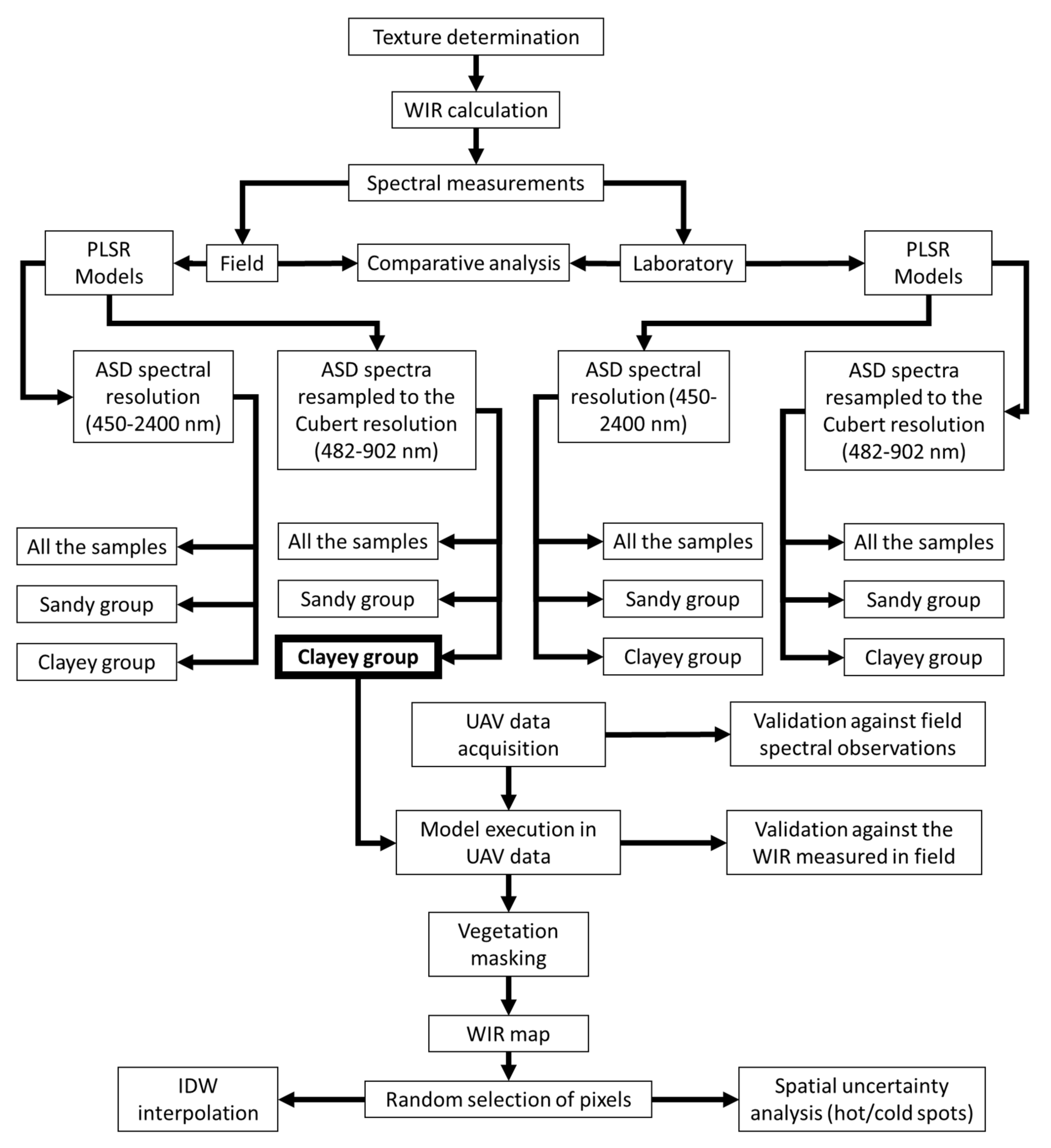
Before running the field spectral-based model on a selected group of soil samples to predict the WIR values in a spatial domain, we removed all pixels that represented vegetation by using the green–red vegetation index, whereas bare soil pixels can be represented by negative values [56]. Figure 3 shows the location of the Alento study area, and an RGB mosaic composed of the Cubert UHD-185 data over this area with the exact locations of the field samples. It is important to note that several pixels were masked out due to the vegetation cover. To represent green light, we considered the reflectance at 550 nm, and for red light, 670 nm. In Figure 3, these pixels are encoded in red. In total, 223,094 pixels represented the bare soil (“red areas”) from a total of 1,463,322 pixels.

For a visual and spatial representation of the WIR distribution, we applied the inverse distance weighting (IDW) interpolation method [57] to the 21 ground-measured WIR values at the Alento study site. We then randomly selected 100 bare soil pixels (from the 223,094 pixels) to reapply the IDW interpolation to the spectral-based WIR predictions. Thus, less samples enable producing a smoother interpolation because a more homogeneous distribution of the points is generated. To perform these interpolations, we selected the default configurations of ArcGIS [57]. As this spatial-based representation cannot be considered a robust validation, and to identify significant concentrations of low and/or high WIR values in the study area, we also applied the Getis-Ord Gi* (pronounced G-i star) method [35,36] to the ground samples and to the 100 bare soil pixels that were randomly selected from the extracted layer of the spectral-based model. The Getis-Ord Gi* method identifies significant hot/cold spots as a function of the analyzed values and the neighboring entities. Thus, if the 21 field samples are not enough for a robust spatial analysis, the Getis-Ord Gi* method can identify robust interpretations in the 100 bare soil pixels selected from the spectral-based WIR predictions. Certainly, this is valid after validation of the UAV data calibration and the spectral similarities between the field and UAV data (Section 2.3). To further validate the UAV spectral-based predictions, we evaluated the correlation between the WIR measured in the field against the WIR predicted from the UAV images after the execution of the spectral-based model for five selected soil samples that were not part of the model calibration and whose assigned pixels were not covered by vegetation.

2.7. Flowchart

Figure 4 provides a flowchart of all of the work phases. This flowchart starts with the texture classification and WIR measurements performed in the field. This is followed by the acquisition of spectral measurements in the field and the laboratory. At both levels (field and laboratory), spectral-based models are generated for the different soil-texture groups and the different spectral configurations: ASD and Cubert. The obtained performance was then compared at every stage, and the spectral-based model that was found to be most indicative was then run on the Cubert hyperspectral image. Note that the selected model was the one created with the clayey group using the Cubert spectral resolution, marked in bold in Figure 4. This decision is further explained and justified in Section 3 and Section 4. Consequently, the flowchart presents the validation phases, vegetation removal, and spatial analyses. In short, it demonstrates the methodological stages from field WIR measurements to UAV spectral-based mapping of the WIR.

3. Results

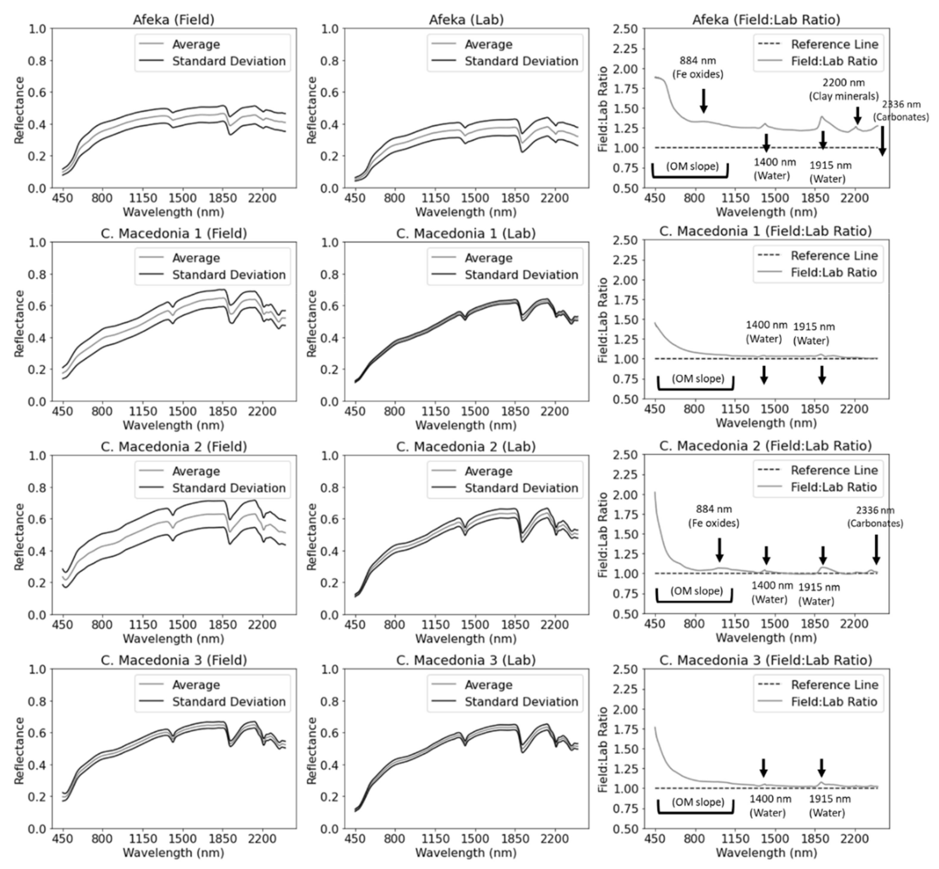
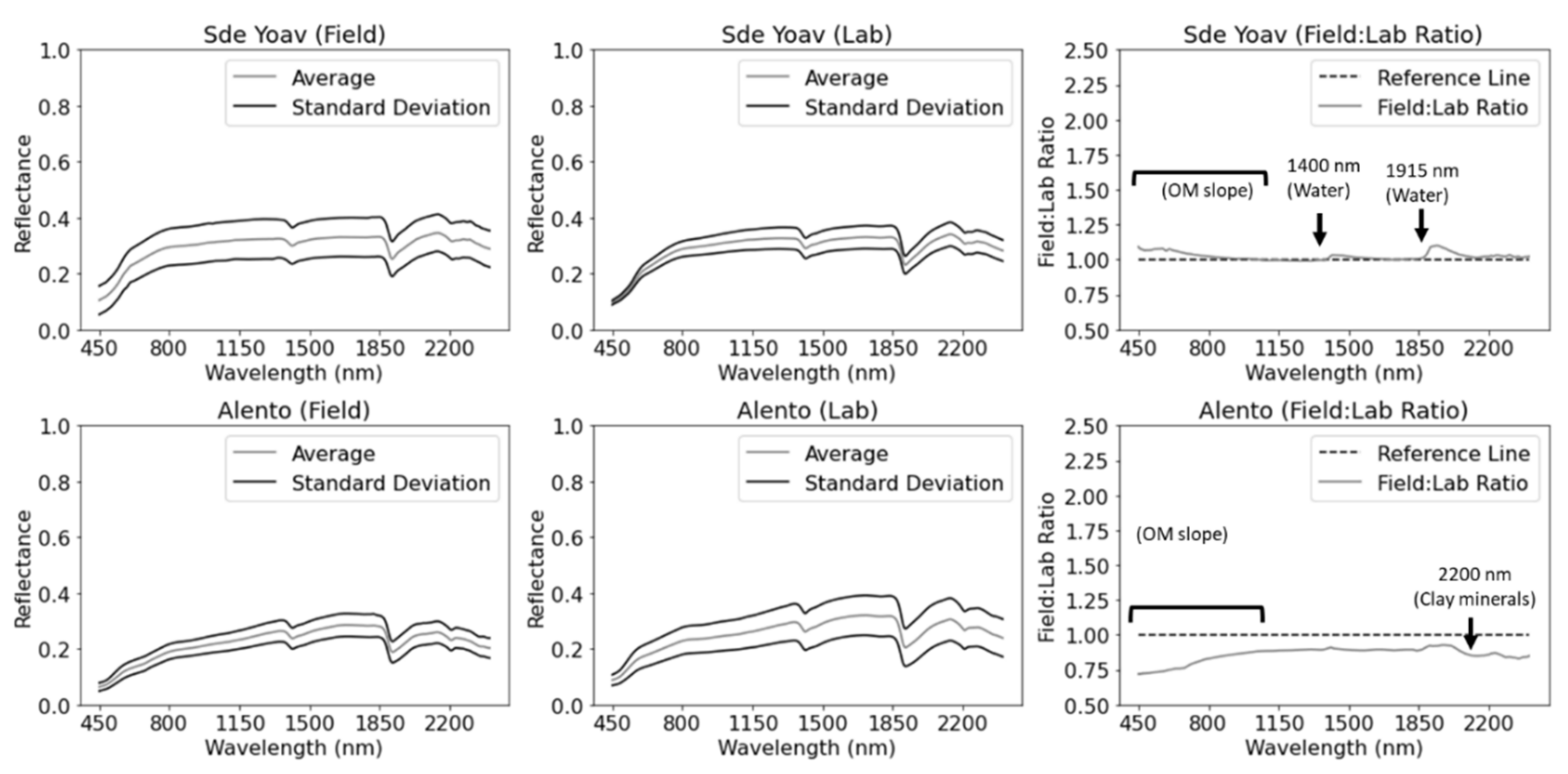
3.1. Spectral Characteristics Per Field

Figure 5 and Figure 6 show the average spectra at each of the selected sites as measured in the laboratory and in the field. In addition, the ratio between these two measurements (field vs. laboratory) is given. Figure 5 illustrates the sandy fields, and the clayey fields are shown in Figure 6. Although in every field the laboratory and field average reflectance appear to be similar, the average spectral ratio between the field and laboratory observations indicated that several spectral features were distorted due to the sampling procedures. In all sandy fields (Figure 5), the average spectral ratio between the field and laboratory observations showed the highest gap in the VNIR spectral range, which can be assigned to the decomposed OM content that decreases the VNIR reflectance as the OM content increases. However, the OM content in the soil surface differed from the soil underneath by color and structure. This effect is also known as the OM spectral slope [26]. In addition, there were some changes in water absorption at 1400 and 1915 nm [46], probably due to the drying process after collecting the samples. Differences in carbonate absorption at around 2336 nm [46] could be observed in the fields of Afeka and Central Macedonia 2. In the Afeka study site (sandy group), the spectral features that can be assigned to hygroscopic water, Fe oxides (884 nm), clay minerals (2200 nm), and carbonate content (2336 nm) were further distorted probably because the soil crust in this field was more developed, and therefore more sensitive to the sampling procedures. Some of these distortions were also noticeable in the fields that represent the clayey soils (Figure 6). In Figure 6, the OM slope was again seen to be affected by the sampling procedure in both fields: Sde Yoav and Alento. Nevertheless, Sde Yoav also showed differences in hygroscopic water absorption, compared to Alento, which showed differences in the clay mineral absorption at 2200 nm. These observations demonstrated that small spectral changes between field and laboratory conditions are mainly due to the sampling procedure.

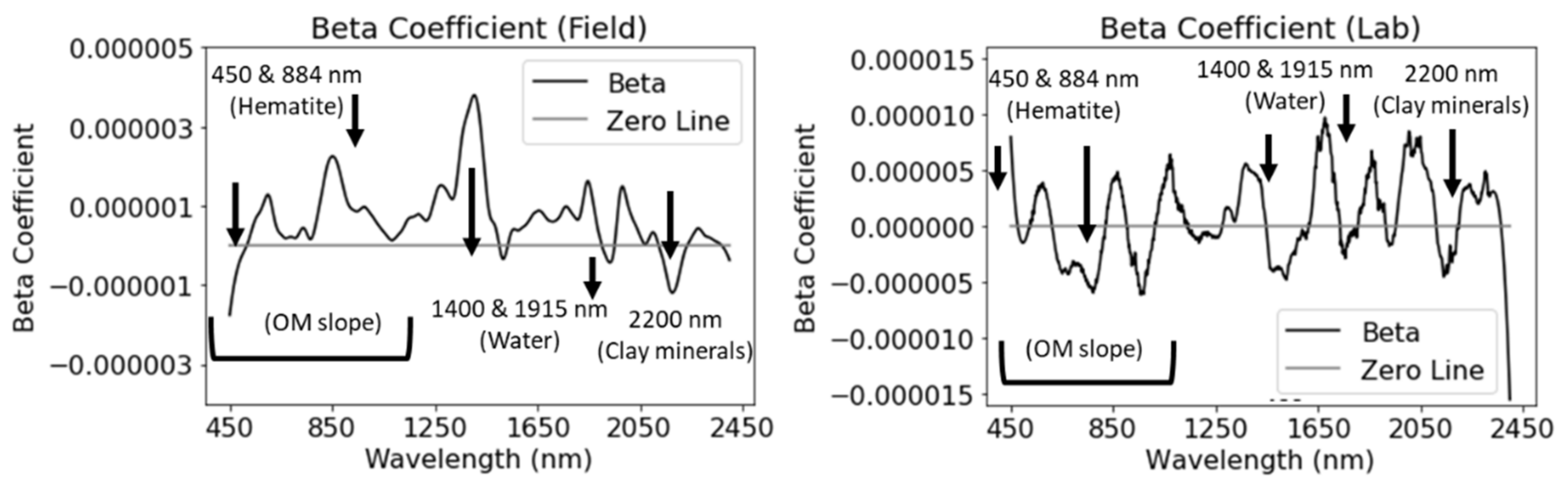
3.2. Spectral-Based Modeling and Interpretation

This section introduces the results of the field and laboratory spectral-based models that were generated using the whole dataset, as well as the clayey and sandy groups separately, with the ASD across the 450–2400 nm spectral region; it also presents the performance of these datasets after being resampled to the spectral configuration of the Cubert UHD-185 (482–902 nm).

Table 2. Dispersion statistics of the studied groups.

Group	Parameter	Value (cm/s)
Whole dataset	Mean	0.00134
	Standard deviation	0.00076
	Interquartile range	0.00075–0.00183
	Skewness	0.44
	Kurtosis	−0.3
	WIR range	0.00007–0.00355
Sandy dataset	Mean	0.001533
	Standard deviation	0.00078
	Interquartile range	0.00091–0.00204
	Skewness	0.4
	Kurtosis	0.49
	WIR range	0.00008–0.00355
Clayey dataset	Mean	0.00111
	Standard deviation	0.00065
	Interquartile range	0.000570.00155
	SkewnessKurtosis	0.25
	Kurtosis	0.83
	WIR range	0.00007–0.00249

WIR, water infiltration rate.

and

Table 3. Dispersion statistics per field.

Group	Field	Parameter	Value (cm/s)
Sandy dataset	Afeka	Mean	0.0013
		Standard deviation	0.00061
		Interquartile range	0.00085–0.00171
		Skewness	0.03557
		Kurtosis	−0.82087
		WIR range	0.00021–0.0025
	C. Macedonia 1	Mean	0.00202
		Standard deviation	0.00079
		Interquartile range	0.00139–0.00254
		Skewness	−0.41873
		Kurtosis	−0.91797
		WIR range	0.00064–0.00324
	C. Macedonia 2	Mean	0.00178
		Standard deviation	0.00085
		Interquartile range	0.00109–0.00235
		Skewness	0.21709
		Kurtosis	−0.66361
		WIR range	0.00043–0.00355
	C. Macedonia 3	Mean	0.00108
		Standard deviation	0.00046
		Interquartile range	0.00077–0.00134
		Skewness	−0.22813
		Kurtosis	−0.33763
		WIR range	0.00008–0.00182
Clayey dataset	Sde Yoav	Mean	0.00143
		Standard deviation	0.00057
		Interquartile range	0.00109–0.00179
		Skewness	−0.06322
		Kurtosis	−0.65508
		WIR range	0.00023–0.00249
	Alento	Mean	0.00056
		Standard deviation	0.00037
		Interquartile range	0.00016–0.00088
		Skewness	0.26864
		Kurtosis	−1.15855
		WIR range	0.00007–0.00119

WIR, water infiltration rate.

show the dispersion statistics of the WIR values that were measured in the field for the whole dataset and each texture group (Table 2) and for each field individually (Table 3). The texture groups differed to quite a large extent. In some cases, the clayey fields such as Sde Yoav presented higher WIR values than the sandy fields, such as Central Macedonia 3 and Afeka. Certainly, texture is one of the most important factors affecting WIR. Accordingly, the variation between soils from the same texture group may be related to other secondary factors, such as OM or minerology. In all cases, the kurtosis and skewness were lower than 1, indicating near-Gaussian distributions [58]. Nonetheless, because we used the PLSR algorithm, the distribution behavior is not expected to play a role in the analysis because PLSR is known to also be effective with non-Gaussian distributions [48,49,50,51].

Table 4. Statistical parameters of the spectral-based models before spectral resampling (450–2400 nm).

Group	Parameter	Field	Laboratory
Whole dataset	RPIQ (Cal)	10.83	5.26
	R2 (Cal)	0.98	0.92
	RMSE (Cal)	0.0001	0.0002
	No. of samples (Cal)	83	83
	RPIQ (Val)	2.26	1.87
	R2 (Val)	0.70	0.57
	RMSE (Val)	0.0004	0.0004
	No. of samples (Val)	21	21
	p-Value (Val)	0.0000	0.0001
	No. of components	9	9
	Spectral preprocessing	1st derivative
Sandy dataset	RPIQ (Cal)	4.24	1.8
	R2 (Cal)	0.90	0.48
	RMSE (Cal)	0.0002	0.22
	No. of samples (Cal)	46	46
	RPIQ (Val)	3.19	1.84
	R2 (Val)	0.82	0.22
	RMSE (Val)	0.0004	0.0007
	No. of samples (Val)	12	12
	p-Value (Val)	0.0001	0.123
	No. of components	5	5
	Spectral preprocessing	Absorbance and 1st derivative
Clayey dataset	RPIQ (Cal)	17.66	4.96
	R2 (Cal)	0.99	0.89
	RMSE (Cal)	5.86	0.0002
	No. of samples (Cal)	37	37
	RPIQ (Val)	3.14	2.85
	R2 (Val)	0.81	0.7
	RMSE (Val)	0.0003	0.0004
	No. of samples (Val)	9	9
	p-Value (Val)	0.0004	0.0025
	No. of components	6	6
	Spectral preprocessing	1st derivative

Val, validation; Cal, calibration.

and

Table 5. Statistical parameters of the spectral-based models after spectral resampling (482–902 nm).

Group	Parameter	Field	Laboratory
Whole dataset	RPIQ (Cal)	2.26	2.05
	R2 (Cal)	0.52	0.41
	RMSE (Cal)	0.0005	0.0006
	No. of samples (Cal)	83	83
	RPIQ (Val)	1.06	1.02
	R2 (Val)	0.36	0.30
	RMSE (Val)	0.0007	0.0007
	No. of samples (Val)	21	21
	p-Value (Val)	0.0038	0.0106
	No. of components	10	10
	Spectral preprocessing	Absorbance and 1st derivative
Sandy dataset	RPIQ (Cal)	2.36	2.59
	R2 (Cal)	0.63	0.55
	RMSE (Cal)	0.0005	0.0005
	No. of samples (Cal)	46	46
	RPIQ (Val)	2.7	1.66
	R2 (Val)	0.83	0.45
	RMSE (Val)	0.0003	0.0005
	No. of samples (Val)	12	12
	p-Value (Val)	0.0000	0.0169
	No. of components	11	11
	Spectral preprocessing	Absorbance and 1st derivative
Clayey dataset	RPIQ (Cal)	2.26	2.05
	R2 (Cal)	0.66	0.47
	RMSE (Cal)	0.0004	0.0005
	No. of samples (Cal)	37	37
	RPIQ (Val)	3.67	2.18
	R2 (Val)	0.86	0.49
	RMSE (Val)	0.0003	0.0005
	No. of samples (Val)	9	9
	p-Value (Val)	0.0001	0.0048
	No. of components	6	6
	Spectral preprocessing	1st derivative

Val, validation; Cal, calibration.

summarize the statistical parameters of all of the models generated before (ASD) and after the spectral resampling (Cubert), respectively. Following these tables, the results extracted from each examined group are interpreted separately, at the field and laboratory levels, in both spectral configurations (ASD and Cubert).

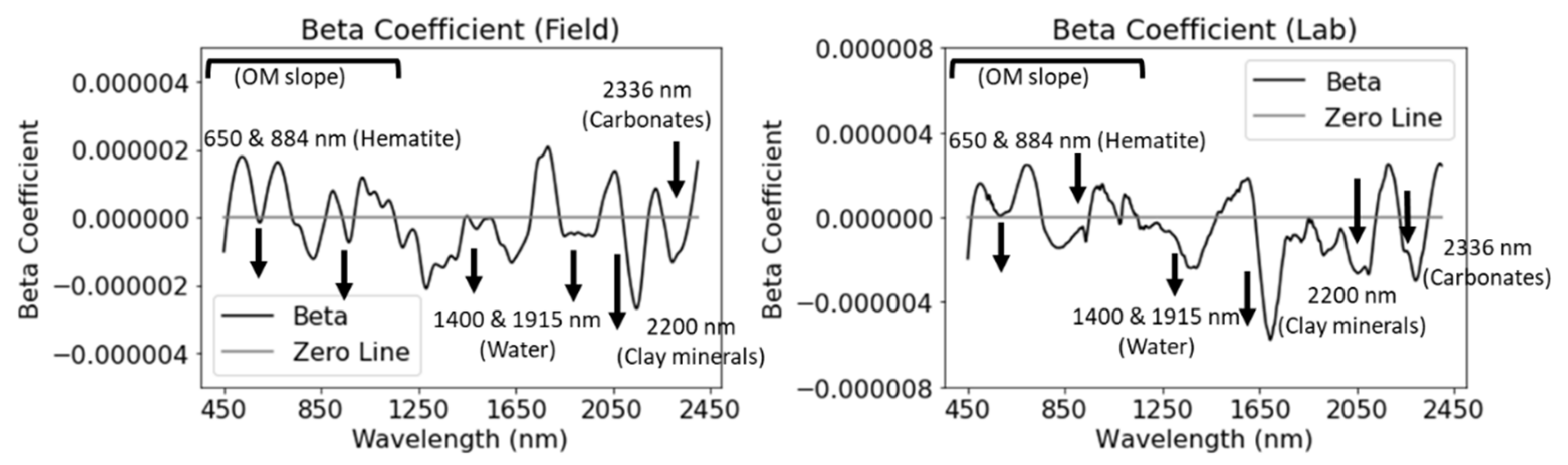
3.2.1. The Whole Dataset in the ASD Spectral Configuration

To generate the spectral-based models to extract WIR from the whole dataset before spectral resampling, the spectral data were submitted to SG first derivative preprocessing using nine components. Execution of the spectral-based model with the calibration group showed high accuracies at both field and laboratory levels (R²_Cal = 0.98 and 0.92, respectively). In the subsequent validation stage, the PLSR models generated using this dataset showed excellent results in the field domain (R²_Val = 0.70). Although the validation of the laboratory-based model showed acceptable performance (R²_Val = 0.57), these results indicated that the field-based model was more effective using the 450–2400 nm spectral range, as expected. Table 4 presents these results.

With this dataset, the beta coefficients of the field- and laboratory-based models showed differences (Figure 7). In the field domain, more extreme positive values were obtained at around 450, 884, 1400, and 2200 nm. Whereas the beta coefficients around 450 nm and 884 nm can be assigned to hematite, the 1400 nm value may be caused by an overtone of the fundamental absorptions of O–H in hygroscopic water and hydroxyl in the chemical structures of clay minerals. The 2200 nm value can be assigned to clay minerals [26,46]. On the other hand, although the beta coefficients of the laboratory-based model highlighted similar spectral features, these were not as well differentiated as in the field-based model.

3.2.2. The Whole Dataset in the Cubert Spectral Configuration

Table 5 presents the results of the PLSR models of both field and laboratory spectral measurements using the whole dataset after spectral resampling (to the Cubert UHD-185 spectral configuration) against the WIR values measured in the field (see Section 2). We used 10 components for both models, where the spectral data were first converted to apparent absorbance and then the SG first derivative was calculated. The accuracies obtained after the execution of the spectral-based model with the calibration group were unsatisfactory at both field and laboratory levels (R²_Cal = 0.52 and 0.41, respectively). In the validation stage, despite the fact that the performance of the whole dataset after resampling was unsatisfactory (in the laboratory and in the field), the field-based model still presented a better correlation than the laboratory-based model (R²_Val = 0.36 and 0.30, respectively). Although the field-based model provided better results, it demonstrated that the contribution of the SWIR spectral range is very important; the VNIR spectral range was insufficient to generate a good generic spectral-based model.

In the whole dataset after spectral resampling, the beta coefficients of the field-based model highlighted the wavelengths between 482 and 650 nm that can be associated with hematite (Fe oxides) [46] and with the OM slope of the VNIR spectral range [26] (Figure 8). On the other hand, in the laboratory-based model, the spectral features around 490 nm could be related to goethite (Fe oxide) content [46], as well as to the OM slope of the VNIR spectral range [26]. Both models highlighted to a small extent the hematite spectral feature at around 884 nm.

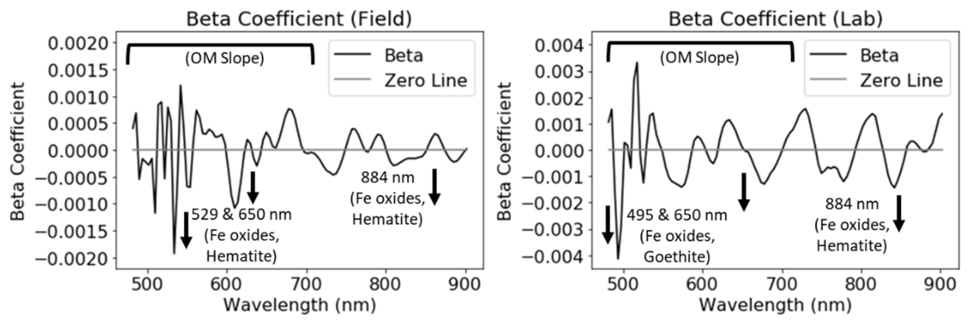
3.2.3. Sandy Dataset in the ASD Spectral Configuration

As already discussed, WIR is strongly affected by soil texture [12,13]. Accordingly, we split the dataset into sandy and clayey groups. For the spectral-based models generated to predict WIR using the ASD spectral resolution (VNIR–SWIR1–SWIR2), the spectral data of the sandy group were transformed into apparent absorbance, and then the SG first derivative was calculated. For the PLSR algorithm at this stage, we used five components. The predictions obtained after execution of the spectral-based model with the calibration group showed higher accuracies at the field vs. laboratory level (R²_Cal = 0.90 and 0.48, respectively). Again, validation of the field-based model showed a better correlation than the laboratory-based model (R²_Val = 0.82 and 0.22, respectively). See Table 4 for the results and statistics.

In general, the beta coefficients for the laboratory- and field-based models of the sandy dataset seemed to present similar spectral features, with no important differences (Figure 9). Nevertheless, in the field domain, extreme beta coefficient values were present in the clay mineral absorption at around 2200 nm. On the other hand, the extreme beta coefficient values in the laboratory model were present in the water absorption at around 1915 nm.

3.2.4. Sandy Dataset in the Cubert Spectral Configuration

At this stage, the ASD spectral data of the sandy group were resampled to the spectral configuration of the Cubert UHD-185 sensor. Before generating the spectral-based models, the spectra were submitted to SG first derivative pretreatment of apparent absorbance. For these PLSR models, we used 11 components. Table 5 provides the results of this analysis. The predictions obtained with the calibration group showed acceptable accuracies at the field and laboratory levels (R²_Cal = 0.63 and 0.55, respectively). Again, validation of the field-based model for the sandy group (after resampling) showed a much better correlation than that of the laboratory-based model (R²_Val = 0.83 and 0.45, respectively).

The beta coefficients of the laboratory and field spectral-based models both showed spectral features that can be associated with the OM slope in the VNIR region (Figure 10). Although both domains showed spectral features related to Fe oxides, they differed in the spectral–mineralogical association. Whereas in the field domain, the most dominant bands were at around 529 and 650 nm and could be assigned to hematite, the laboratory spectral-based model emphasized the bands at around 495 and 650 nm that can be related to goethite, and the bands at around 884 that can be associated to hematite. Note that according Viscarra Rossel and Bahrens [46], absorption around 650 nm can be related to both hematite and goethite.

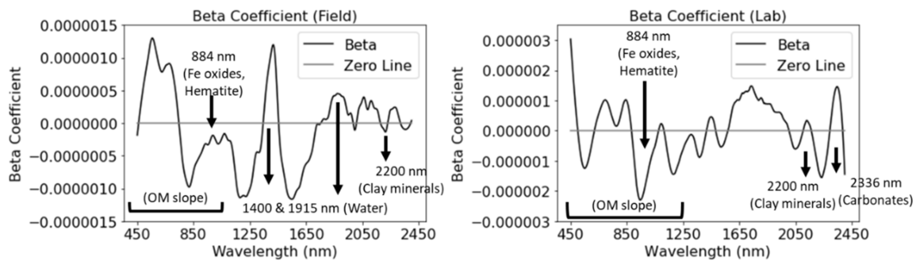
3.2.5. Clayey Dataset in the ASD Spectral Configuration

For the PLSR models that were created to assess the WIR using the clayey dataset, the spectral data were transformed with the SG first derivative, and six components were used to calibrate the models. Both laboratory- and field-based models presented excellent accuracies in the calibration groups (R²_Cal = 0.99 and 0.89, respectively), as well as in the validation groups using the full spectral range (VNIR–SWIR) of the ASD (R²_Val = 0.81 and = 0.70, respectively), where the field-based model still presented better results (Table 4).

The laboratory- and field-based models generated using the clayey dataset presented beta coefficients that in general differed (Figure 11). Both the laboratory- and field-based models emphasized the visible spectral region up to around 600 nm, but the field-based model also considered the region up to around 750 nm. These features can be related to the spectral features of Fe oxides and the OM slope in the VNIR spectral range, especially in the field-based model [26]. As seen in Figure 11, in the clayey group, the field-based model mostly took advantage of spectral features at around 1400 nm, which can be caused by hygroscopic water. On the other hand, the laboratory-based model emphasized spectral features at around 884 nm, which can be assigned to OM, hygroscopic water, or Fe oxides [26,46]. This gap may be caused by the water-retention properties of OM [59,60,61] and by the fact that OM tends to accumulate over the undisturbed soil surface due to animal and plant biological activity. Once the samples were brought to the laboratory, the quantitative characteristics of the OM slope in the VNIR spectral range may have declined because the soil surface had been disturbed. Thus, the laboratory-based spectral model had to be calibrated from other spectral features. In addition, the laboratory model emphasized bands related to the carbonate content at 2336 nm.

3.2.6. Clayey Dataset in the Cubert Spectral Configuration

The clayey dataset was resampled to the Cubert UHD-185 spectral configuration. The reflectance data were preprocessed using the SG first derivative, and six components were used to generate the PLSR model. Table 5 illustrates the results of the resampled clayey dataset. The performance obtained in the field was much better than that obtained in the laboratory for both calibration (R²_Cal = 0.66 and 0.47, respectively) and validation groups (R²_Val = 0.86 and 0.49, respectively).

In the spectrally resampled clayey dataset, the beta coefficients of the field-based model emphasized the 482–650 nm spectral range, which can be related to the OM slope in the VNIR region or to geothite (Fe oxides) (Figure 12). Nevertheless, as the other Fe oxide spectral features were not as dominant in the field domain, we can assume that the OM slope was the dominant element in calibrating the field spectral model since OM is present in the soil surface. The laboratory-based model gave much more importance to all used spectra (VNIR) in general, with accentuation of the 482–550 nm and 870–902 nm spectral ranges, which can be attributed to hematite spectral features at around 529, 650, and 884 nm, respectively. Certainly, all of the spectral features at the laboratory level could also be associated with OM, but as the hematite spectral absorptions were very dominant at this level, we assume that these contributed more than the OM spectral features because the sampling procedure destroys the soil surface where the OM content is higher.

From these results, it was postulated that field observations are better for predicting WIR and that splitting the dataset into clayey and sandy soil groups provides better accuracy. This is because for each texture, the soil surface behaves differently. It is thus recommended that for spectral prediction of WIR, the soil texture be evaluated in the field [45], and then an FSSL that is represented by this texture must be executed using spectral-based models. The explanations for the spectral assignments resulting from the ASD and Cubert UHD-185 spectral resolutions (VNIR–SWIR and VNIR, respectively) could be similar. Due to sampling procedures, the quantitative spectral properties of the OM slope may decrease in the laboratory domain. Therefore, the laboratory-based model was forced to use different chromophores to estimate WIR. Both hematite and goethite are products of different stages of the pedogenesis process, starting in the upper layers of the soil surface, which are affected by rain, erosion, biological activity, etc. Whereas goethite is more dominant in the initial stages of soil formation, hematite is generated at more advanced phases under dry conditions [62]. Therefore, the beta coefficients resulting from the field- and laboratory-based models demonstrate that soil surface-dependent properties as well as the aging stage of the soil, are disturbed by the sampling procedure. Among the resampled datasets, the field-based model of the clayey dataset provided the best performance and better represented the texture of the Alento study site. Thus, this spectral-based model was selected for further utilization of the UAV–Cubert hyperspectral sensor in a spatial domain in the following steps.

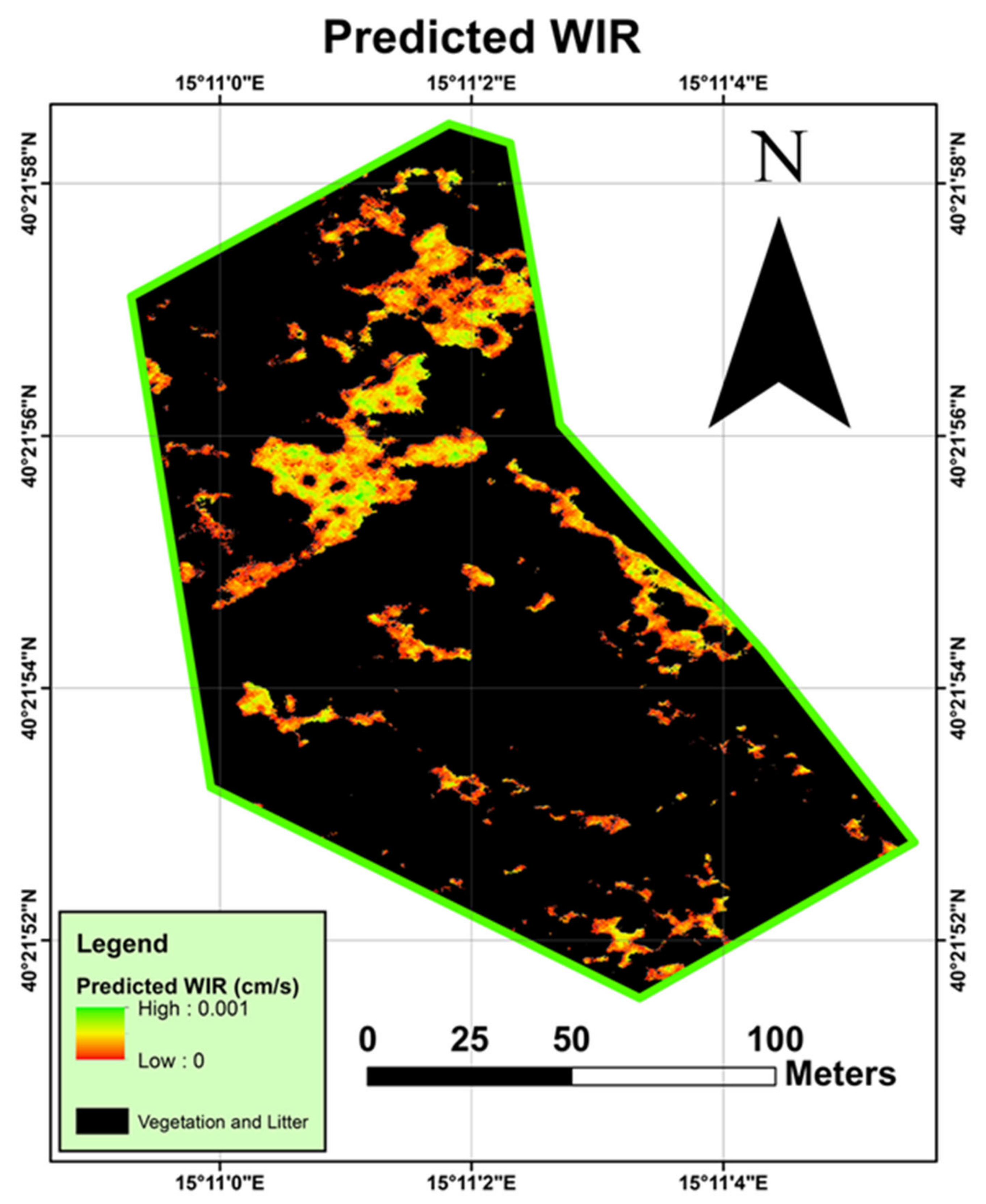
3.3. Execution of the Field-Based Model with the Cubert UHD-185 Data

Based on the results of the spectral-based models that demonstrated a strong dependency on soil texture in predicting WIR, we selected the model that was created using the clayey group (after resampling to the Cubert UHD-185 spectral configuration) for application to the UAV hyperspectral data. The result of the spectral-based model’s execution over the bare soil pixels is shown in Figure 13 where the vegetation and litter pixels were masked out using the green-red vegetation index [56].

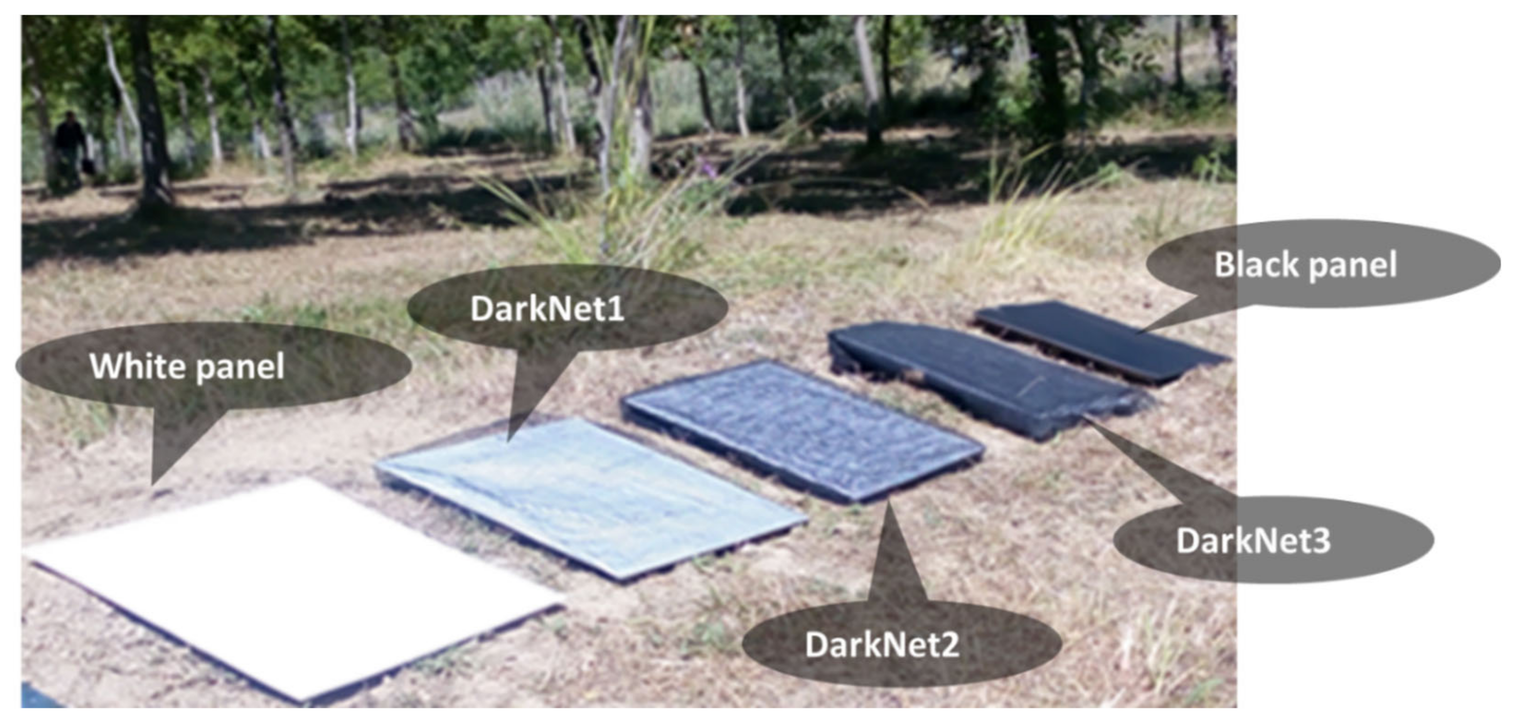
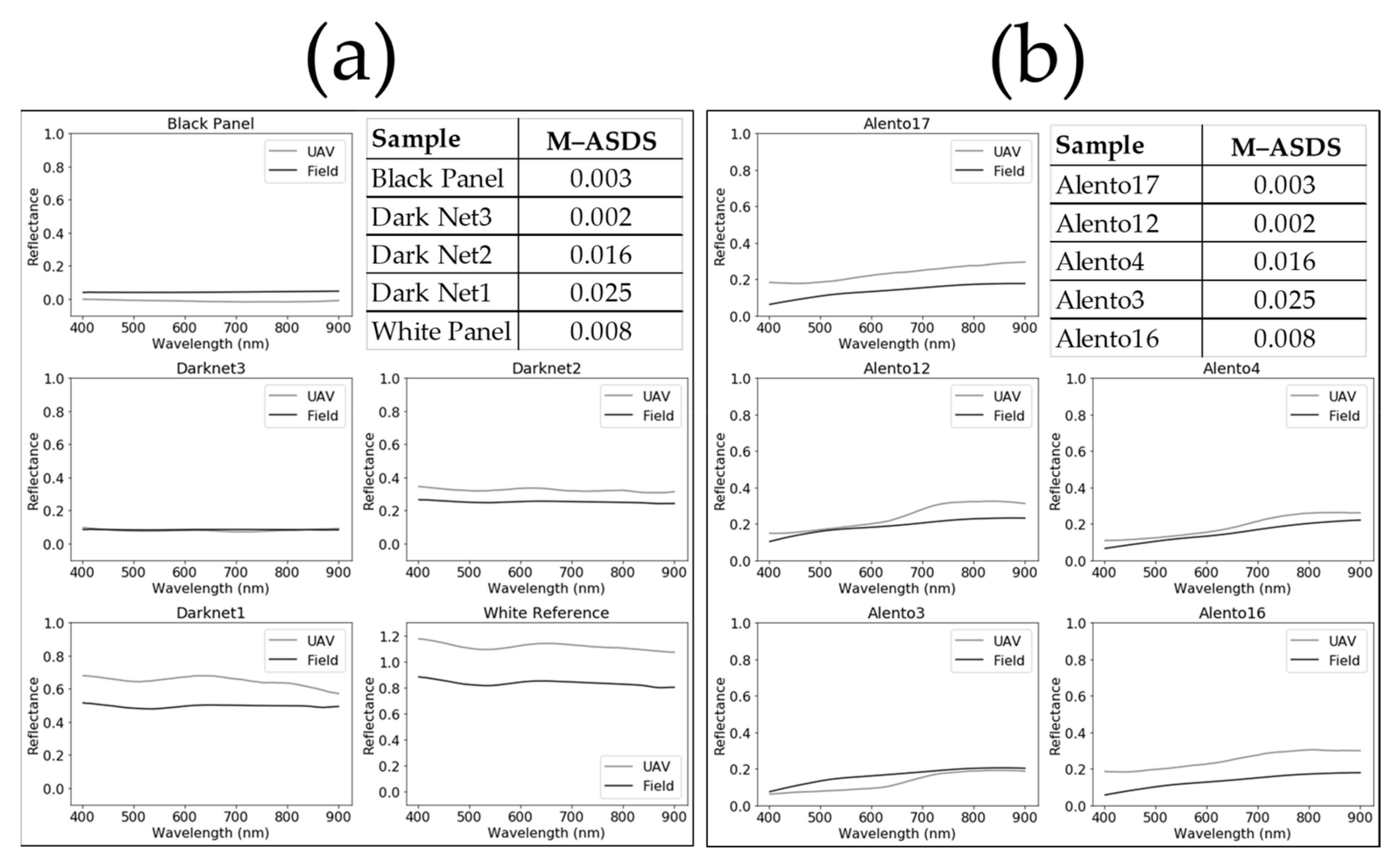
3.3.1. Validation of the UAV Reflectance Calibration and WIR Predictions

The calibration of the UAV reflectance data from the Cubert DN image was described in Section 2. The UAV reflectance calibration was validated by measuring several ground targets with the SoilPRO assembly (see Section 2.3). Figure 14 presents the calibrated reflectance of the Cubert within the corresponding reflectance measured in the field. Figure 14a shows the reference panels, and Figure 14b shows the bare soil targets. These figures also present the M–ASDS values to judge the similarity between the ground and UAV measurements (described in Section 2.5). Low M–ASDS values suggest a good match between a spectral pair. As seen in Figure 14a, the spectra were visually well matched, with low M–ASDS values ranging from 0 to 0.024 (2.4%) that indicated high spectral similarity and fair atmospheric correction of the Cubert data. The soil field spectra (Figure 14b) were also similar to the UAV spectra (in Figure 14b), although in "Alento12", a weak chlorophyll feature at around 670 nm was observed. We assume that this effect occurred because the pixel was slightly mixed with canopy, litter, and/or vegetation, while it was measured by the Cubert sensor as the UAV view (and angle) differed from the SoilPRO perspective in the field, which used clean soils. Still, all of the soil samples presented M–ASDS values below 0.025, which indicate a good match with errors below 2.5% [63]. As seen in Figure 14, the spectral similarities and the low M–ASDS values presented by the validation panels and the field samples strongly confirm the reliability of the spectral reflectance extracted from the Cubert for the entire bare soil of Alento.

To quantitatively validate the predictions of the Cubert WIR map, we performed in situ ground truth measurements over bare soil targets at the Alento study site where the WIR was measured with the infiltrometer. These samples were not part of the calibration phase of the selected model. The predicted WIR values presented by the pixels at the coordinates of these targets were extracted, and the predicted WIR values were plotted against the WIR field measurements. This plot is shown in Figure 15. Certainly, five soil samples may not be a robust number to perform an “external” validation test for the UAV predictions. Due to the vegetation coverage (87%), it was not possible to find more reliable samples that were bare, exposed to the sun and not part of the calibration group.

These samples acted more as ground truth samples to account for the trend of the spectral-based model and the correlation shows quite satisfactory results with the expected trend.

Table 6. Statistical performance of the spectral-based model that was selected to run on the Cubert reflectance image.

Parameter	Value
RPIQ (Val)	2.61
R2 (Val)	0.76
RMSE (Val)	0.0002
No. of samples (Val)	5
p-Value (Val)	0.052
Spectral range	482–902 nm
WIR range (cm/s)	0.00007–0.00014

summarizes this relationship, with the statistical parameters presented by the spectral-based model that was executed on the UAV image.

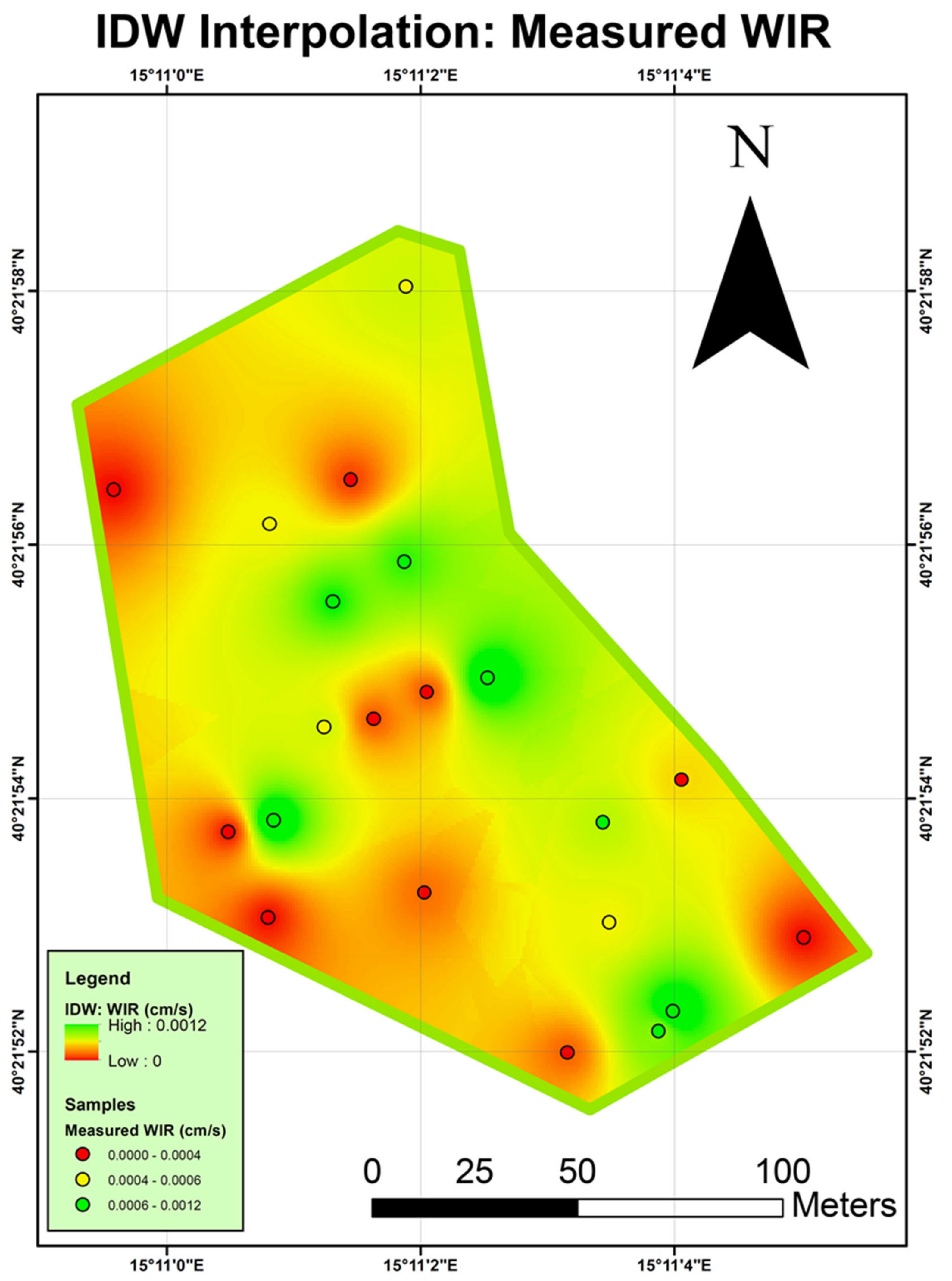
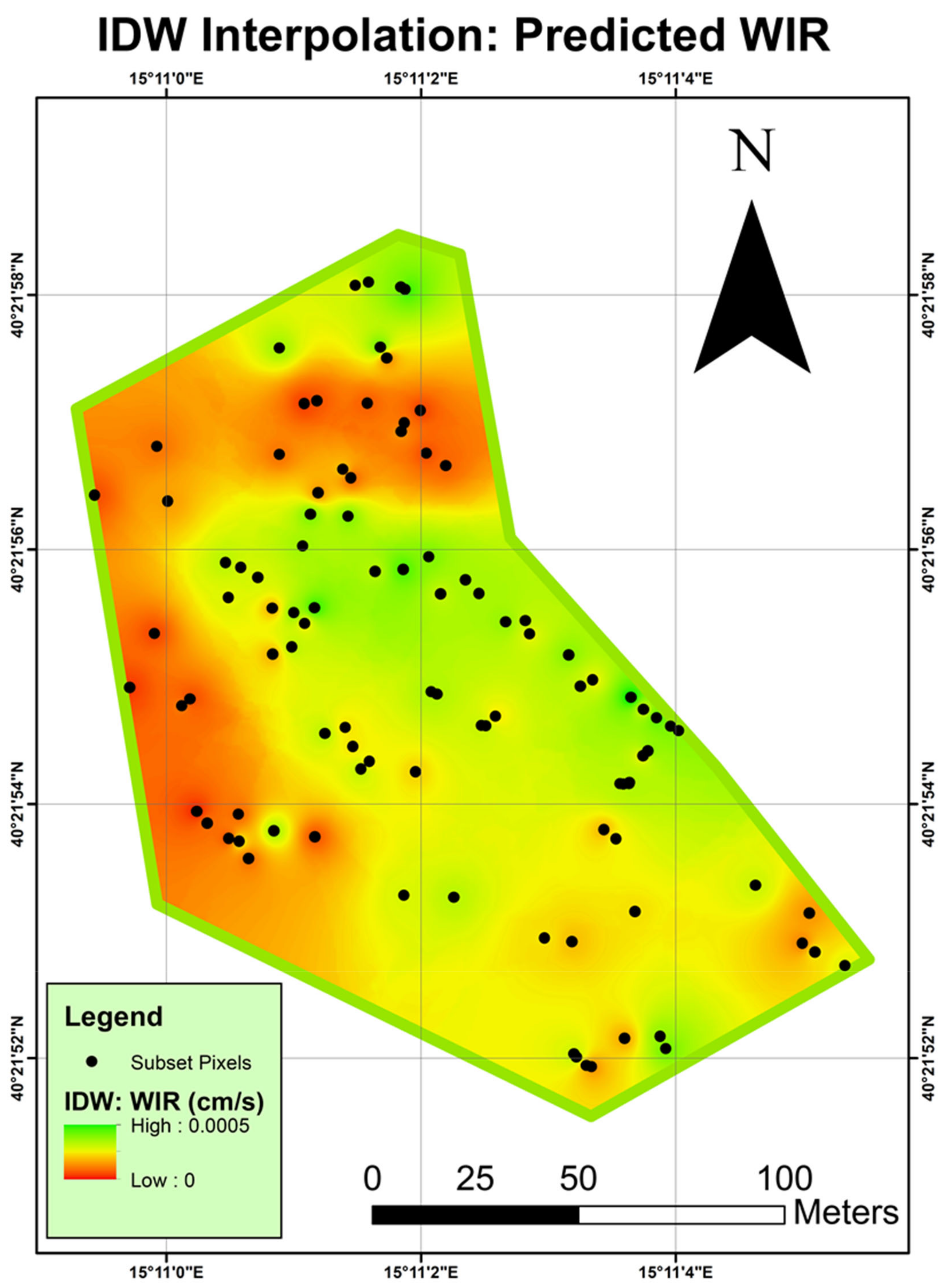
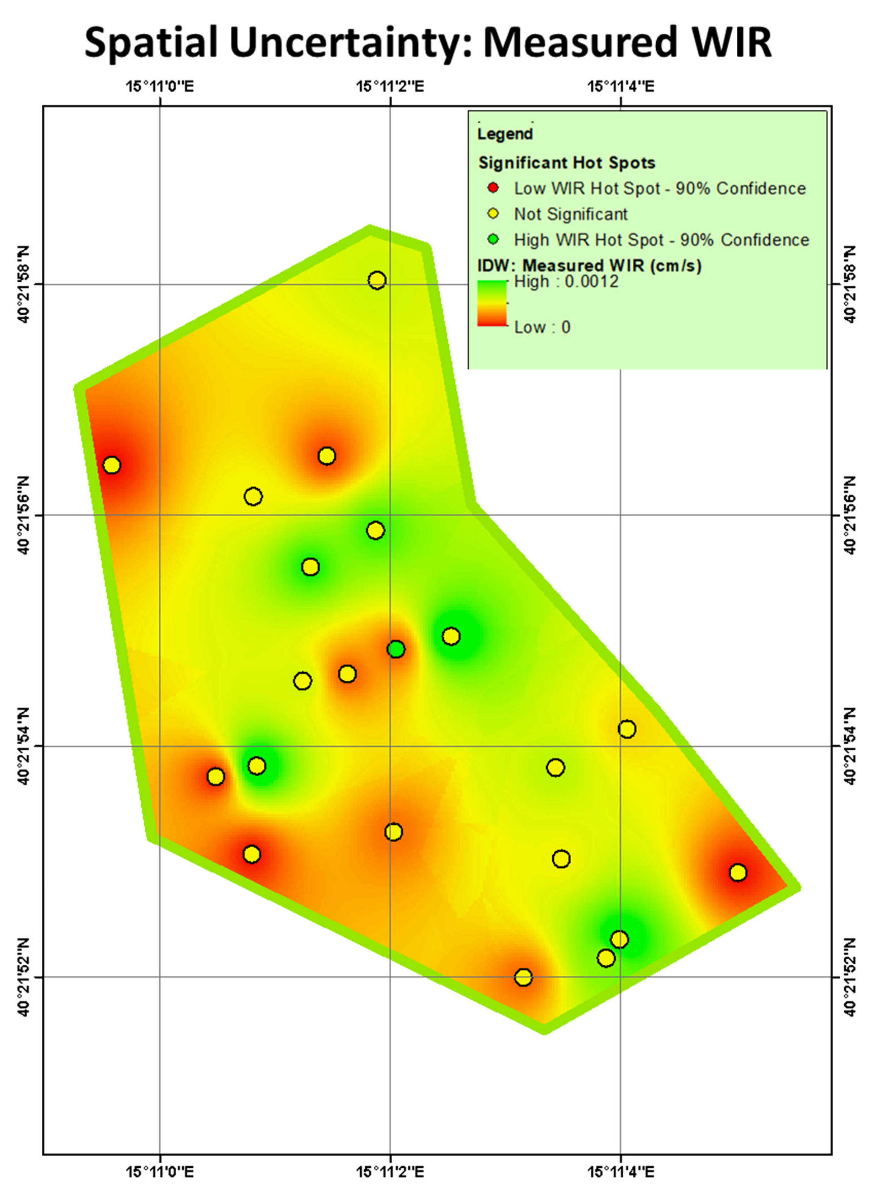
3.3.2. Spatial and Uncertainty Analyses

For a spatial representation of the WIR distribution, we applied the IDW interpolation method to the 21 field samples in the Alento study site (Figure 16). Nevertheless, as the map in Figure 16 is based on interpolation of only 21 samples, it was assumed that more samples are needed to better represent the WIR spatial distribution. Thus, as the bare soil pixels underwent a WIR estimation using the clayey spectral-based model, we applied a second IDW interpolation to 100 pixels (from a total of 223,094 bare soil pixels) that were randomly selected from the respective soil pixels of the spectral-based WIR predictions (Figure 17).

To verify this assumption, as well as the uncertainty of the spatial dependency of the WIR, we calculated the Getis-Ord Gi* statistic [35,36] for each sample in both cases:

I.

The WIR measured in situ with the 21 samples (Figure 18)

II.

The predicted WIR in the selected exposed soil pixels, containing 100 samples/pixels (Figure 19).

As shown in Figure 18, most of the samples that were measured in the field were classified as non-significant, whereas there was one sample that was classified as a hot spot with high WIR (erroneously) despite a very low measured WIR. This error might have been caused by the high WIR values of the neighboring samples, as shown in the interpolation of Figure 18. On the other hand, in Figure 19, where more samples were extracted from the spectral-based predictions (100 pixels), higher degrees of confidence (>90%) were obtained. This is also noticeable in pixels located in areas with very low (red) or very high (green) WIR. Certainly, 21 samples are not sufficient to perform a good interpolation in this study area, and the Cubert WIR image contributed a great deal of information toward minimizing the uncertainty. As shown in Figure 19, when many more samples were used with better spatial distribution, a fair identification of hot spots of both high and low WIR was obtained with high certainty in the Cubert WIR image. This emphasizes the need for technologies, such as spectral imaging, to enlarge the number of observations that are well distributed across the exposed soil areas in order to obtain a more reliable picture of the property in question.

4. Discussion

4.1. Influence of Sampling Procedures on the Soil Surface

This study was aimed at developing a simple and rapid method to map WIR on a pixel-by-pixel basis, rather than relying on a few traditional WIR measurements executed in the field. To that end, soil reflectance spectroscopy was used at the laboratory, field, and aerial levels. The study was conducted in sequential stages that investigated the discrepancies between field and laboratory spectral observations using different soil-texture groups. As expected, all of the field-based models at all levels provided better accuracy than the laboratory-based ones. The analyzed beta coefficients revealed that the quantitative spectral properties of clay minerals, Fe oxides, and OM may be lost when the soil samples are collected for laboratory testing.

This confirmed the assumption that soil sampling is a destructive method that modifies the field condition, which is doubly important: First, for the WIR measurements, and second, for the RS view that sees only the upper thin surface layer of the soil. In clayey soils, the surface seal is well developed and structured based on clay–clay, clay–OM, clay–Fe oxide, and clay-CaCO₃ interactions, all of which are affected by raindrop energy, whereas this effect is smaller in sandy soils [64]. As accumulated raindrop energy organizes soil particle sizes in the upper layers of the soil [14,15], bringing the lower-weight particles to the top, disturbance of the soil crust can result in the replacement of hematite spectral features with those of others, such as goethite, as seen in the case of the sandy group. On the other hand, in the clayey group, sampling procedures annulled the contribution of the OM slope to the VNIR spectral range so that the spectral-based model could detect other spectral features.

Soil-sampling procedures in the field, which are essential for laboratory spectral measurements, lead to the loss of spectral features that are relevant to the thin surface characteristics. Accordingly, the results of this study pinpoint the importance of using high-quality field spectral information to represent the aerial RS view. This practice is essential for monitoring sensitive soil surface properties such as WIR. Other relevant soil surface-dependent properties might include soil water repellency, soil salinity, and soil biogenic crust status [33].

4.2. The Potential of Soil Surface Reflectance and the SoilPRO Assembly

In all of the datasets, we demonstrated the need for caution in analyzing soil surface-dependent properties. This emphasizes the capacity of the SoilPRO (or similar) assembly to derive soil surface reflectance without disturbing the thin soil layer. The SoilPRO not only preserves the surface condition, it is also unaffected by atmospheric attenuation and changes in the sun’s angle, resulting in stable and standardized results. As RS means can only monitor the soil surface (penetrating to around 50 µm), it is strongly recommended that the SoilPRO (or similar) assembly be used for ground-truth measurements as well as for modeling soil surface-related properties [33].

4.3. Spectral Range and Resolution

As demonstrated in the first part of this study that evaluated the gap between field and laboratory spectral observations, we obtained better results in the field domain, regardless of whether the samples were classified as sandy or clayey, even when evaluating a generic approach for all samples. Moreover, even when evaluating performance in the field and laboratory domains using different spectral resolutions (ASD and Cubert UHD-185), the field-based models presented better results. Although a generic model that utilizes all soil textures can be extracted from the VNIR–SWIR spectral range, dividing the soils into clayey and sandy groups provided better results. It should be noted that to adapt the spectral data to the spectral configuration of the Cubert UHD-185, we used only the VNIR spectral region, which is quite limited in terms of soil spectral fingerprints. The ASD’s spectral resolution across the entire optical region provides more information by including the contribution of the SWIR spectral region. It is thus assumed that airborne hyperspectral imagers that cover the entire VNIR–SWIR spectral range will provide better and more accurate WIR maps.

4.4. Vegetation Cover

The Alento study site had a lot of vegetation and litter coverage during the Cubert UHD-185 flight, with approximately 13% bare soil pixels. Even though all of the samples were collected from bare soil, not all of them were exposed to the UAV sensor’s view due to the UAV angle perspective and to canopy coverage. Interpolation of the WIR data over the clean soil pixels provided us with predictions of the WIR under the canopy. However, the accuracy of these interpolations requires further investigation because soil cover is one of the main factors controlling water penetration into the soil [65]. As seen in Figure 16, Figure 17, Figure 18 and Figure 19, the IDW interpolations of the measured (21 points) and predicted (100 points) WIR values seemed to illustrate a similar spatial distribution of WIR. Moreover, several hotspots of high and low WIR were identified with high confidence in the interpolation of the 100 predicted values of the selected pixels. Therefore, the predicted WIR in areas under the canopy may be reasonable, because the interpolation of the predicted WIR was based on bare soil pixels. It is likely that if the bare soil is exposed to the sensor view and there is no vegetation, the accuracy will be higher, as all of the pixels can undergo spectral-based modeling. Nonetheless, vegetation is obviously common in agricultural fields, and this exercise demonstrated that it is possible to deliver a reliable WIR map by interpolating the exposed soil pixels.

4.5. Future Studies and Remarks

Although we used a hyperspectral sensor that was limited in its spectral range (VNIR region), new light hyperspectral sensors that cover the entire VNIR–SWIR region are emerging. This technology onboard UAV platforms combined with high spatial resolution capability can improve the WIR mapping results. This is because field spectral-based models of high resolution (including the SWIR range) that contain more spectral information can then be implemented. This direction is not only valid for the WIR property, but could be aligned with other soil surface properties, such as OM. Further studies might be executed with larger FSSLs obtained using the SoilPRO assembly or similar techniques, to cover more soil types from different parts of the world. It should be pointed out that this case study is only a proof of concept for rapid WIR mapping using field spectroscopy. Such maps are important for the control of runoff and soil erosion, as well as for increasing water penetration into the root zone. Once a WIR map can be rapidly generated, the farmer can use it to destroy the hard soil seals prior to a rain event and, accordingly, obtain less erosion and save water. To that end, further effort should be made to expand the FSSLs worldwide and to direct activity to form new FSSLs in parallel to the traditional SSLs, which are widely available today. The new hyperspectral era of RS technologies may foster such an idea.

Nevertheless, due to the vegetation coverage, it was not possible to use more than five reliable samples for the ground truth examination of the WIR values predicted from the UAV spectral data. Still, despite the high vegetation coverage of the Alento study site, this work demonstrated the possibility to map the WIR from an UAV platform using bare soil pixels that were available to the sensor view. This achievement was possible mainly because we executed careful field reflectance measurements that preserve the surface conditions. Accordingly, we believe that this work paves the way to improve the monitoring of soil surface-related properties (and not only WIR) using HRS means onboard UAV, airborne and satellite platforms.

5. Conclusions

The results of this study lead us to conclude that several spectral properties were lost and/or distorted in the laboratory due to the sampling procedure, which disrupted the soil surface and biased the prediction of the WIR using laboratory measurements as the WIR is very sensitive to the surface conditions. These discrepancies were mainly manifested in the clay mineral, OM, and Fe oxide spectral properties. As WIR is a soil surface-dependent property, spectral-based models benefit more from field than laboratory spectral data in the assessment of WIR in the soil. Obtaining FSSLs using assemblies such as the SoilPRO can overcome this problem because they provide (real) field measurements of undisturbed soils with laboratory quality. Separating the soil samples into clayey and sandy groups provided better spectral-based models for estimating the WIR values using the field-based models in all spectral ranges and configurations (ASD and Cubert). Applying the field spectral-based model to the Cubert–UAV data gave reasonable results that were successfully validated.

Nonetheless, in the future we recommend carrying out similar studies with more field samples for a deeper examination of the possibility of mapping the WIR using FSSLs and UAV spectral imaging platforms. Vegetation coverage might be a problem, but after filtering it out from the image, the Getis-Ord Gi* method identified significant hot/cold spots of WIR in the study area upon analysis of the UAV data. Further studies based on this work should be applied with a sensor that covers the whole optical range with higher spectral resolutions, and FSSLs should be expanded worldwide, as is already the case for traditional SSLs, to study soil surface-dependent properties at any site.

References

1. Franzluebbers, A.J. Water infiltration and soil structure related to organic matter and its stratification with depth. Soil Tillage Res. 2002, 66, 197–205. [Google Scholar] [CrossRef]
2. Basche, A.D.; DeLonge, M.S. Comparing infiltration rates in soils managed with conventional and alternative farming methods: A meta-analysis. PLoS ONE 2019, 14, e0215702. [Google Scholar] [CrossRef] [Green Version]
3. Wilcox, B.P.; Wilding, L.P.; Woodruff, C.M. Soil and topographic controls on runoff generation from stepped landforms in the Edwards Plateau of Central Texas. Geophys. Res. Lett. 2007, 34. [Google Scholar] [CrossRef] [Green Version]
4. Rietkerk, M.; van de Koppel, J. Alternate stable states and threshold effects in semi-arid grazing systems. Oikos 1997, 79, 69–76. [Google Scholar] [CrossRef] [Green Version]
5. Thurow, T.L.; Blackburn, W.H.; Taylor, C.A., Jr. Hydrologic characteristics of vegetation types as affected by livestock grazing systems, Edwards Plateau, Texas. J. Range Manag. 1986, 39, 505–509. [Google Scholar] [CrossRef]
6. Thurow, T.L.; Blackburn, W.H.; Taylor, C.A., Jr. Infiltration and interrill erosion responses to selected livestock grazing strategies, Edwards Plateau, Texas. J. Range Manag. 1988, 41, 296–302. [Google Scholar] [CrossRef]
7. Van de Koppel, J.; Rietkerk, M.; Weissing, F.J. Catastrophic vegetation shifts and soil degradation in terrestrial grazing systems. Trends Ecol. Evol. 1997, 12, 352–356. [Google Scholar] [CrossRef] [Green Version]
8. Van de Koppel, J.; Rietkerk, M.; van Langevelde, F.; Kumar, L.; Klausmeier, C.A.; Fryxell, J.M.; Hearne, J.W.; van Andel, J.; de Ridder, N.; Skidmore, A.; et al. Spatial heterogeneity and irreversible vegetation change in semiarid grazing systems. Am. Nat. 2002, 159, 209–218. [Google Scholar] [CrossRef]
9. Walker, B.H.; Ludwig, D.; Holling, C.S.; Peterman, R.M. Stability of semi-arid savanna grazing systems. J. Ecol. 1981, 69, 473–498. [Google Scholar] [CrossRef]
10. Moody, J.A.; Kinner, D.A.; Úbeda, X. Linking hydraulic properties of fire-affected soils to infiltration and water repellency. J. Hydrol. 2009, 379, 291–303. [Google Scholar] [CrossRef]
11. Lado, M.; Paz, A.; Ben-Hur, M. Organic matter and aggregate size interactions in infiltration, seal formation, and soil loss. Soil Sci. Soc. Am. J. 2004, 68, 935–942. [Google Scholar] [CrossRef]
12. Stern, R.; Benhur, M.; Shainberg, I. Clay mineralogy effect on rain infiltration, seal formation and soil losses. Soil Sci. 1991, 152, 455–462. [Google Scholar] [CrossRef]
13. Ben-Hur, M.; Letey, J. Effect of polysaccharides, clay dispersion, and impact energy on water infiltration. Soil Sci. Soc. Am. J. 1989, 53, 233–238. [Google Scholar] [CrossRef]
14. Agassi, M.; Morin, J.; Shainberg, I. Effect of raindrop impact energy and water salinity on infiltration rates of sodic soils. Soil Sci. Soc. Am. J. 1985, 49, 186–190. [Google Scholar] [CrossRef]
15. Agassi, M.; Bloem, D.; Ben-Hur, M. Effect of drop energy and soil and water chemistry on infiltration and erosion. Water Resour. Res. 1994, 30, 1187–1193. [Google Scholar] [CrossRef]
16. Bertrand, A.R.; Sor, K. The effects of rainfall intensity on soil structure and migration of colloidal materials in soils. Soil Sci. Soc. Am. J. 1962, 26, 297–300. [Google Scholar] [CrossRef]
17. Levy, G.J.; van der Watt, H.v.H. Effects of clay mineralogy and soil sodicity on soil infiltration rate. S. Afr. J. Plant. Soil 1988, 5, 92–96. [Google Scholar] [CrossRef]
18. Bullard, J.E.; Ockelford, A.; Strong, C.; Aubault, H. Effects of cyanobacterial soil crusts on surface roughness and splash erosion. J. Geophys. Res. Biogeosci. 2018, 123, 3697–3712. [Google Scholar] [CrossRef]
19. Six, J.; Elliott, E.T.; Paustian, K. Soil structure and soil organic matter II. A normalized stability index and the effect of mineralogy. Soil Sci. Soc. Am. J. 2000, 64, 1042–1049. [Google Scholar] [CrossRef]
20. Nadler, A.; Levy, G.J.; Keren, R.; Eisenberg, H. Sodic calcareous soil reclamation as affected by water chemical composition and flow rate. Soil Sci. Soc. Am. J. 1996, 60, 252–257. [Google Scholar] [CrossRef]
21. Nimmo, J.R. Aggregation: Physical Aspects. In Reference Module in Earth Systems and Environmental Sciences; Elsevier: Amsterdam, The Netherlands, 2013; ISBN 978-0-12-409548-9. [Google Scholar]
22. Angers, D.A.; Caron, J. Plant-induced changes in soil structure: Processes and feedbacks. Biogeochemistry 1998, 42, 55–72. [Google Scholar] [CrossRef]
23. Vaezi, A.R.; Ahmadi, M.; Cerdà, A. Contribution of raindrop impact to the change of soil physical properties and water erosion under semi-arid rainfalls. Sci. Total Environ. 2017, 583, 382–392. [Google Scholar] [CrossRef]
24. Morin, J.; Goldberg, D.; Seginer, I. A rainfall simulator with a rotating disk. Trans. ASAE 1967, 10, 74–77. [Google Scholar] [CrossRef]
25. Decagon Devices, Inc. Minidisk Infiltrometer; User’s Manual; Decagon Devices, Inc: Pullman, WA, USA, 2005. [Google Scholar]
26. Ben-Dor, E. Quantitative remote sensing of soil properties. Adv. Agron. 2002, 75, 173–243. [Google Scholar]
27. Viscarra Rossel, R.A.; Behrens, T.; Ben-Dor, E.; Brown, D.J.; Demattê, J.A.M.; Shepherd, K.D.; Shi, Z.; Stenberg, B.; Stevens, A.; Adamchuk, V.; et al. A global spectral library to characterize the world’s soil. Earth Sci. Rev. 2016, 155, 198–230. [Google Scholar] [CrossRef] [Green Version]
28. Tóth, G.; Jones, A.; Montanarella, L. The LUCAS topsoil database and derived information on the regional variability of cropland topsoil properties in the European Union. Environ. Monit. Assess. 2013, 185, 7409–7425. [Google Scholar] [CrossRef]
29. Tziolas, N.; Tsakiridis, N.; Ben-Dor, E.; Theocharis, J.; Zalidis, G. A memory-based learning approach utilizing combined spectral sources and geographical proximity for improved VIS-NIR-SWIR soil properties estimation. Geoderma 2019, 340, 11–24. [Google Scholar] [CrossRef]
30. Ogen, Y.; Zaluda, J.; Francos, N.; Goldshleger, N.; Ben-Dor, E. Cluster-based spectral models for a robust assessment of soil properties. Geoderma 2019, 340, 175–184. [Google Scholar] [CrossRef]
31. Ben-Dor, E.; Goldshleger, N.; Braun, O.; Kindel, B.; Goetz, A.F.H.; Bonfil, D.; Margalit, N.; Binaymini, Y.; Karnieli, A.; Agassi, M. Monitoring infiltration rates in semiarid soils using airborne hyperspectral technology. Int. J. Remote Sens. 2004, 25, 2607–2624. [Google Scholar] [CrossRef]
32. Goldshleger, N.; Ben-Dor, E.; Chudnovsky, A.; Agassi, M. Soil reflectance as a generic tool for assessing infiltration rate induced by structural crust for heterogeneous soils. Eur. J. Soil Sci. 2009, 60, 1038–1051. [Google Scholar] [CrossRef]
33. Ben-Dor, E.; Granot, A.; Notesco, G. A simple apparatus to measure soil spectral information in the field under stable conditions. Geoderma 2017, 306, 73–80. [Google Scholar] [CrossRef]
34. Romano, N.; Nasta, P.; Bogena, H.; De Vita, P.; Stellato, L.; Vereecken, H. Monitoring hydrological processes for land and water resources management in a Mediterranean ecosystem: The Alento River Catchment Observatory. Vadose Zone J. 2018, 17, 1–12. [Google Scholar] [CrossRef] [Green Version]
35. Ord, J.K.; Getis, A. Local spatial autocorrelation statistics: Distributional issues and an application. Geogr. Anal. 1995, 27, 286–306. [Google Scholar] [CrossRef]
36. Getis, A.; Ord, J.K. The analysis of spatial association by use of distance statistics. Geogr. Anal. 1992, 24, 189–206. [Google Scholar] [CrossRef]
37. Su, Z.; Zeng, Y.; Romano, N.; Manfreda, S.; Francés, F.; Ben Dor, E.; Szabó, B.; Vico, G.; Nasta, P.; Zhuang, R.; et al. An integrative information aqueduct to close the gaps between satellite observation of water cycle and local sustainable management of water resources. Water 2020, 12, 1495. [Google Scholar] [CrossRef]
38. Paruta, A.; Ciraolo, G.; Capodici, F.; Manfreda, S.; Sasso, S.F.D.; Zhuang, R.; Romano, N.; Nasta, P.; Ben-Dor, E.; Francos, N.; et al. A geostatistical approach to map near-surface soil moisture through hyperspatial resolution thermal inertia. IEEE Trans. Geosci. Remote Sens. 2020, 1–18. [Google Scholar] [CrossRef]
39. Rubel, F.; Kottek, M. Observed and projected climate shifts 1901-2100 depicted by world maps of the Köppen-Geiger climate classification. Meteorol. Z. 2010, 135–141. [Google Scholar] [CrossRef] [Green Version]
40. Costantini, E.A.C.; Dazzi, C. The Soils of Italy; Springer Science & Business Media: Berlin, Germany, 2013; ISBN 978-94-007-5642-7. [Google Scholar]
41. Ravikovitch, S. The Soils of Israel: Formation, Nature and Properties; Hakibbutz Hameuchad Publication House: Bnei Brak, Israel, 1992. [Google Scholar]
42. Ravikovitch, S. Manual and Map of Soils of Israel; The Magnes Press, The Hebrew University: Jerusalem, Israel, 1969. [Google Scholar]
43. Soil Map of Greece—ESDAC—European Commission. Available online: https://esdac.jrc.ec.europa.eu/content/soil-map-greece-0 (accessed on 27 October 2019).
44. Ben Dor, E.; Ong, C.; Lau, I.C. Reflectance measurements of soils in the laboratory: Standards and protocols. Geoderma 2015, 245–246, 112–124. [Google Scholar] [CrossRef]
45. Thien, S.J. A flow diagram for teaching texture-by-feel analysis. J. Agronom. Educ. 1979, 8, 54–55. [Google Scholar] [CrossRef]
46. Viscarra Rossel, R.A.; Behrens, T. Using data mining to model and interpret soil diffuse reflectance spectra. Geoderma 2010, 158, 46–54. [Google Scholar] [CrossRef]
47. Wold, S.; Sjöström, M.; Eriksson, L. PLS-regression: A basic tool of chemometrics. Chemom. Intell. Lab. Syst. 2001, 58, 109–130. [Google Scholar] [CrossRef]
48. Schamberger, T.; Schuberth, F.; Henseler, J.; Dijkstra, T.K. Robust partial least squares path modeling. Behaviormetrika 2020, 47, 307–334. [Google Scholar] [CrossRef] [Green Version]
49. Dijkstra, T.K.; Henseler, J. Consistent and asymptotically normal PLS estimators for linear structural equations. Comput. Stat. Data Anal. 2015, 81, 10–23. [Google Scholar] [CrossRef] [Green Version]
50. Hair, J.F.; Hult, G.T.M.; Ringle, C.M.; Sarstedt, M.; Thiele, K.O. Mirror, mirror on the wall: A comparative evaluation of composite-based structural equation modeling methods. J. Acad. Market. Sci. 2017, 45, 616–632. [Google Scholar] [CrossRef]
51. Takane, Y.; Hwang, H. Comparisons among several consistent estimators of structural equation models. Behaviormetrika 2018, 45, 157–188. [Google Scholar] [CrossRef]
52. Zhao, D.; Arshad, M.; Wang, J.; Triantafilis, J. Soil exchangeable cations estimation using Vis-NIR spectroscopy in different depths: Effects of multiple calibration models and spiking. Comput. Electron. Agric. 2021, 182, 105990. [Google Scholar] [CrossRef]
53. Pedregosa, F.; Varoquaux, G.; Gramfort, A.; Michel, V.; Thirion, B.; Grisel, O.; Blondel, M.; Prettenhofer, P.; Weiss, R.; Dubourg, V.; et al. Scikit-Learn: Machine Learning in Python. J. Mach. Learn. Res. 2011, 12, 2825–2830. [Google Scholar]
54. Bellon-Maurel, V.; Fernandez-Ahumada, E.; Palagos, B.; Roger, J.-M.; McBratney, A. Critical review of chemometric indicators commonly used for assessing the quality of the prediction of soil attributes by NIR spectroscopy. Trends Anal. Chem. 2010, 29, 1073–1081. [Google Scholar] [CrossRef]
55. Ben-Dor, E.; Kindel, B.; Goetz, A.F.H. Quality assessment of several methods to recover surface reflectance using synthetic imaging spectroscopy data. Remote Sens. Environ. 2004, 90, 389–404. [Google Scholar] [CrossRef]
56. Motohka, T.; Nasahara, K.N.; Tsuchida, S.; Oguma, H. Applicability of green-red vegetation index for remote sensing of vegetation phenology. Remote Sens. 2010, 2, 2369–2387. [Google Scholar] [CrossRef] [Green Version]
57. IDW—Help. ArcGIS for Desktop. Available online: http://desktop.arcgis.com/en/arcmap/10.3/tools/spatial-analyst-toolbox/idw.htm (accessed on 27 January 2019).
58. George, D.; Mallery, P. IBM SPSS Statistics 23 Step by Step: A Simple Guide and Reference, 14th ed.; Routledge: New York, NY, USA, 2016; ISBN 978-0-13-432025-0. [Google Scholar]
59. Rawls, W.J.; Pachepsky, Y.A.; Ritchie, J.C.; Sobecki, T.M.; Bloodworth, H. Effect of soil organic carbon on soil water retention. Geoderma 2003, 116, 61–76. [Google Scholar] [CrossRef]
60. Olness, A.; Archer, D. Effect of organic carbon on available water in soil. Soil Sci. 2005, 170, 90–101. [Google Scholar] [CrossRef]
61. Saxton, K.E.; Rawls, W.J. Soil water characteristic estimates by texture and organic matter for hydrologic solutions. Soil Sci. Soc. Am. J. 2006, 70, 1569–1578. [Google Scholar] [CrossRef] [Green Version]
62. Inda, A.V.; Fink, J.R.; dos Santos, T.F. Pedogenic iron oxides in soils of the Acre State, Brazil. Ciênc. Rural 2018, 48. [Google Scholar] [CrossRef]
63. Ogen, Y.; Faigenbaum-Golovin, S.; Granot, A.; Shkolnisky, Y.; Goldshleger, N.; Ben-Dor, E. Removing moisture effect on soil reflectance properties: A case study of clay content prediction. Pedosphere 2019, 29, 421–431. [Google Scholar] [CrossRef]
64. Santos, F.; Abney, R.; Barnes, M.; Bogie, N.; Ghezzehei, T.A.; Jin, L.; Moreland, K.; Sulman, B.N.; Berhe, A.A. Chapter 9—The Role of the Physical Properties of Soil in Determining Biogeochemical Responses to Soil Warming. In Ecosystem Consequences of Soil Warming; Mohan, J.E., Ed.; Academic Press: Cambridge, MA, USA, 2019; pp. 209–244. ISBN 978-0-12-813493-1. [Google Scholar]
65. Pingping, H.; Xue, S.; Li, P.; Zhanbin, L. Effect of vegetation cover types on soil infiltration under simulating rainfall. Nat. Environ. Pollut. Technol. 2013, 12, 193–198. [Google Scholar]
Figure 1. (a) Mediterranean basin and the locations of the fields from which the samples were collected. (b) Zoomed in view of the central locations of the fields in Greece.
Remotesensing 13 02606 g001
Figure 2. The validation targets in the agricultural field in Alento, Italy.
Remotesensing 13 02606 g002
Figure 3. RGB image of the study area with the sample collection sites.
Remotesensing 13 02606 g003
Figure 4. Flowchart of the methods followed in this work.
Remotesensing 13 02606 g004
Figure 5. Average reflectance obtained in the field and laboratory and average spectral ratio between field and laboratory spectral measurements (per field) for the sandy group.
Remotesensing 13 02606 g005
Figure 6. Average reflectance obtained in the field and laboratory and average spectral ratio between field and laboratory spectral measurements (per field) for the clayey group.
Remotesensing 13 02606 g006
Figure 7. Beta coefficients of the PLSR models for the prediction of WIR using all samples and the ASD spectral resolution.
Remotesensing 13 02606 g007
Figure 8. Beta coefficients of the PLSR models for the prediction of WIR using all samples, with the resampled data (to the Cubert spectral resolution).
Remotesensing 13 02606 g008
Figure 9. Beta coefficients of the PLSR models for the prediction of WIR using the samples of the sandy group, and the ASD spectral resolution.
Remotesensing 13 02606 g009
Figure 10. Beta coefficients for the prediction of WIR using the samples of the sandy group with the resampled data (to the Cubert spectral resolution).
Remotesensing 13 02606 g010
Figure 11. Beta coefficients of the PLSR models for the prediction of WIR using the samples of the clayey group with the ASD spectral resolution.
Remotesensing 13 02606 g011
Figure 12. Beta coefficients of the PLSR models for the prediction of WIR using the samples of the clayey group with the resampled data (to the Cubert spectral resolution).
Remotesensing 13 02606 g012
Figure 13. The predicted WIR values over the exposed soil pixels and the masked pixels that represent vegetation and/or litter.
Remotesensing 13 02606 g013
Figure 14. Field samples for validation. Gray line, UAV spectrum; black line, field spectrum. (a) Validation panels. (b) Validation soil samples.
Remotesensing 13 02606 g014
Figure 15. Predicted water infiltration rate (WIR) of the validation samples using the Cubert UHD-185 sensor in an UAV.
Remotesensing 13 02606 g015
Figure 16. IDW interpolation of the measured WIR in the field using the 21 measurement points in the field assuming no vegetation.
Remotesensing 13 02606 g016
Figure 17. IDW interpolation of the predicted WIR after execution of the spectral-based model on the exposed soil pixels in the hyperspectral image.
Remotesensing 13 02606 g017
Figure 18. Spatial uncertainty of the WIR field measurements.
Remotesensing 13 02606 g018
Figure 19. Spatial uncertainty of the predicted WIR.
Remotesensing 13 02606 g019