Adaptive Beamforming for Passive Synthetic Aperture with Uncertain Curvilinear Trajectory

Abstract

Recently, numerous reconstruction-based adaptive beamformers have been proposed, which can improve the quality of imaging or localization in the application of passive synthetic aperture (PSA) sensing. However, when the trajectory is curvilinear, existing beamformers may not be robust enough to suppress interferences efficiently. To overcome the model mismatch of unknown curvilinear trajectory, this paper presents an adaptive beamforming algorithm by reconstructing the interference-plus-noise covariance matrix (INCM). Using the idea of signal subspace fitting, we construct a joint optimization problem, where the unknown directions of arrival (DOAs) and array shape parameters are coupled together. To tackle this problem, we develop a hybrid optimization method by combining the genetic algorithm and difference-based quasi-Newton method. Then, a set of non-orthogonal bases for signal subspace is estimated with an acceptable computational complexity. Instead of reconstructing the covariance matrix by integrating the spatial spectrum over interference angular sector, we extract the desired signal covariance matrix (DSCM) directly from signal subspace, and then the INCM is reconstructed by eliminating DSCM from the sample covariance matrix (SCM). Numerical simulations demonstrate the robustness of the proposed beamformer in the case of signal direction error, local scattering and random curvilinear trajectory.

1. Introduction

Passive synthetic aperture (PSA) is a technology that uses time-space correlation of signals and motion information of sensor platform to construct a virtual array, therefore effectively expanding the aperture of sensing system, which can greatly benefit the quality of imaging or localization [1,2]. As one of the most important procedures of synthetic aperture radar (SAR) imaging [3,4], beamforming is a data-dependent array signal processing technique, which aims to extract the desired signal while suppressing interferences from other directions and ambient noise.

Typically, traditional imaging scenario uses conventional beamformer. However, the conventional beamformer is data-independent, which cannot effectively suppress interference. To this end, Capon proposed the well-known standard Capon beamformer (SCB) [5], which can achieve optimal performance when the actual INCM and the steering vector (SV) of desired signal are precisely known. Because the precise INCM is unknown in practical applications, a practical version of SCB named sample covariance matrix inversion (SMI) beamformer was proposed using the sample covariance matrix (SCM), which is highly sensitive to SV mismatches. By applying the diagonal loading technique, Cox proposed a modified version of SCB that joins identity matrix and the SCM together [6]. Several SCM-based beamformers were proposed later, such as the robust capon beamformer (RCB) [7], the worst-case optimization techniques [8,9], the Convex optimization beamforming [10], the linear constrained RCB [11] and the adaptive beamforming algorithm that uses iterative approach [12].

Some works show that when there are SV mismatches, the signal of interest (SOI) component in the SCM will cause performance degradation of the SCM-based beamformers, which is related to the input signal-to-noise ratio (SNR), and when the SNR is high, the performance of SCM-based beamformer may be dramatically reduced due to sell-canceling [13]. To overcome this issue, [14] proposed a covariance matrix reconstruction method using an angular sector reconstruction technique, which is called the reconstruction and estimation beamformer (REB). REB first divides the whole angular domain into two parts, namely the sector of the desired signal and the complement sector that only contains interferences and noise. Then, REB reconstructs the INCM using the nominal SV and spatial spectrum in the complement sector. Based on the concept of INCM reconstruction, plenty of beamformers were proposed, for example, REB with sparse spatial spectrum [15], the low-rank beamformers [16], the subspace-projection-based INCM reconstruction beamformers [17]. In [18], a spatial spectrum estimation method is proposed, which uses the concept of maximum entropy in the procedure of INCM reconstruction, in [19], authors correct the interference SV by estimating gradient vector, which results in more precise INCM. In [20], authors try to remove the desired signal from the received signal, which can lead to a desired-signal-free INCM. In [21], authors shrink the uncertainty set of received signals, and reconstruct the covariance matrix of interference and desired signal. To be robust with SV mismatches due to sensor displacement, Chen et al. applied weighted subspace fitting to SV estimating and then calculates the weighing vector using the reconstructed INCM [22].

The above-mentioned algorithms assume that the sensor locations are exactly known and stay unchanged during the observation procedure. Similarly, when these methods are applied to SAR imaging/localization, the velocity of platform is usually assumed as a constant value with a linear flight path. However, in practical environments, trajectory variations due to atmospheric turbulence or other causes are inevitable. To overcome these challenges, an intuitional idea is to calibrate the sensor position error in the beamforming procedure and estimate the ambient noise power.

In terms of array shape or trajectory calibration, numerous array calibration methods were proposed, and the first type of calibration methods mainly use auxiliary sensors including heading, pose, and depth sensors. Howard et al. [23] estimated the array shape by installing heading sensors at both ends of the horizontal towed array. Park et al. [24] installed multiple heading and pitch sensors in each segment of the horizontal towed line array, and then obtained the array deformation model. However, the accuracy of calibration using auxiliary sensors is severely limited by the accuracy of each sensor. In addition, the auxiliary sensors also require additional channels to collect real-time data, which brings great challenges to the engineering implementation.

When the trajectory changes, the characteristics of virtual array observation data will change accordingly. Using this feature, scholars presented plenty of self-calibration methods. Theoretically, these calibration methods can estimate the array shape without additional types of sensors. In [25], Gary et al. using eigen-decomposition to estimate the phase information of the signals received by each sensor, and then the position of each sensor can be estimated. However, This method needs precisely known incident angles of all signals. Ng et al. [26] prefabricated several reference sources with precisely known DOAs, and coordinated the emission time or frequency of each source. Then the array shape is estimated using the array observation data. To further reduced the number of reference sources, Park et al. [27,28] modeled the sensor position as a polynomial form of angle and array element spacing, and used weighted subspace fitting (WSF) to estimate the sensor positions and array shape.

To be completely free of reference sources, some self-calibration methods were proposed. However, when the reference sources are not used, the signal DOAs are unknown and coupled with the sensor positions in the steering vector (SV) of the array, which will cause ambiguity in sensor position estimation. With regard to this issue, Weiss et al. [29,30] proposed to calculate the sensor positions and DOAs iteratively. For the partially calibrated array, Yang et al. [4] proposed to use the wideband signal received by the hydrophone array to deblur the phase of the SV, then the sensor positions and DOAs can be jointly estimated.

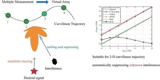
Considering the facts that the performance of existing adaptive beamforming algorithms is far from optimum when the trajectory is curvilinear, this paper proposes a robust curvilinear PSA reconstruction and estimation beamformer (C-PSA-REB), which can enhance the beamformer’s performance in two aspects. The first aspect is that we present signal model when the trajectory is curvilinear in arbitrary plane. The second aspect is that we propose a reconstruction algorithm that can precisely obtain the INCM when the trajectory is curvilinear.

The rest of this paper is organized as follows. In Section 2, we describe the signal model of this paper. In Section 3, we describe the details of the proposed beamforming algorithm. Several numerical examples are simulated, and the results are demonstrated in Section 4. Finally, in Section 5, we draw some conclusions of this paper.

2. Signal Model of Curvilinear Trajectory

In this section, we consider the most fundamental scenario that one sensor with a single channel measures M times continuously during the movement at a distance of d, which equals to a virtual array with M sensors.

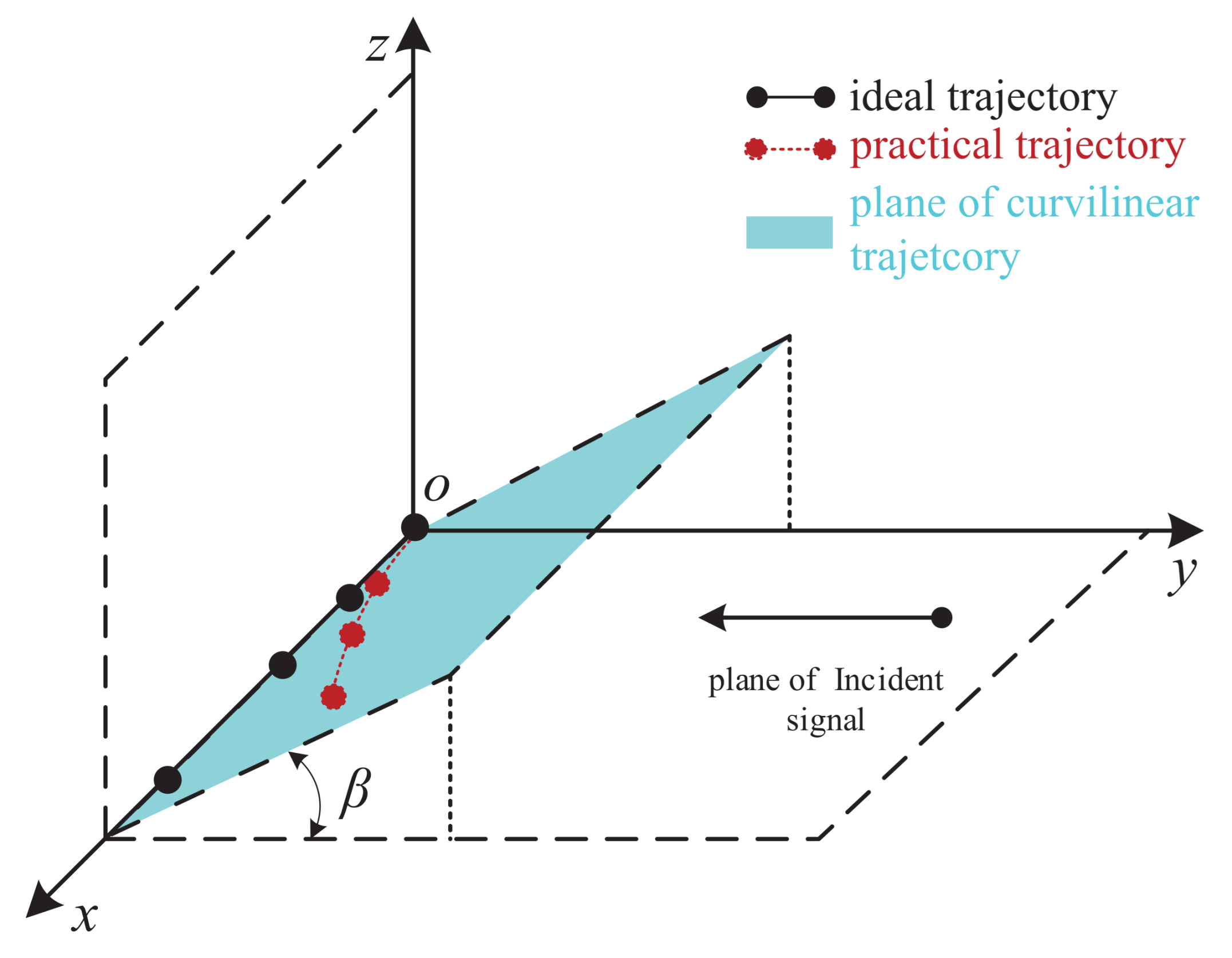
Figure 1 shows the curvilinear trajectory in 3-D view, the ideal trajectory is a strict straight line that is located on the x-axis, and the incident signals are assumed in the xoy plane.

Noticing that the trajectory may be curvilinear due to various causes, and the curved trajectory may be not on the signal incident plane, and the angle between the curved plane and the xoy plane is $\beta$. Figure 2 shows the curvilinear trajectory in the plane of curve, we assume that when the trajectory is curved, the scalar speed of movement is barely changed. In other word, the platform travel distance between two measurements are almost d, and the angle between the m-th and the $m+1$-th measurement are ${\alpha }_m$.

Hence, the coordinates of all virtual sensors can be modeled as

$$\begin{array}{cc}\hfill & p_{x,m+1}=p_{x,m}+dcos{\alpha }_m,\hfill \\ \hfill & p_{y,m+1}=p_{y,m}+dsin{\alpha }_{m}cos\beta ,\hfill \\ \hfill & p_{z,m+1}=p_{z,m}+dsin{\alpha }_{m}cos\beta .\hfill \end{array}$$

(1)

Assume that the first sensor represents the first measurements, which is the reference sensor, the coordinates of the m-th ($m=2,\cdots ,M$) virtual sensor can be approximated in an iterative form as

$$\begin{array}{cc}\hfill & p_{x,m}\approx \sum _{j=1}^{m-1}dcos{\alpha }_j,\hfill \\ \hfill & p_{y,m}\approx \sum _{j=1}^{m-1}dsin{\alpha }_{j}cos\beta ,\hfill \\ \hfill & p_{z,m}\approx \sum _{j=1}^{m-1}dsin{\alpha }_{j}sin\beta .\hfill \end{array}$$

(2)

According to (2), the matrix of all virtual sensors’ coordinates can be defined as [21]

$${\mathbf{P}}_M(\mathit{\alpha },\beta )=\left. [\begin{array}{cccc}0,& p_{x,2},& \cdots ,& p_{x,M}\\ 0,& p_{y,2},& \cdots ,& p_{y,M}\\ 0,& p_{z,2},& \cdots ,& p_{z,M}\end{array}\right]$$

(3)

Hence, the SV of the curvilinear path (virtual array) at direction $\theta$ is described as a function of vector $\mathit{\alpha }={[{\alpha }_1,{\alpha }_2,\cdots ,{\alpha }_M]}^{\mathrm{T}}$ and $\beta$ as

$$\mathbf{a}(\mathit{\alpha },\beta ,\theta )=e^{-j{\mathbf{k}}^{\mathrm{T}}(\theta ){\mathbf{P}}_M(\mathit{\alpha },\beta )},$$

(4)

where $\mathbf{k}(\theta )$ represents the vector of wavenumber, and it is defined as follows

$$\mathbf{k}(\theta )=k_{\mathrm{w}}\mathbf{v}(\theta )={-k_{\mathrm{w}}[cos\theta ,sin\theta ,0]}^{\mathrm{T}},$$

(5)

where $k_{\mathrm{w}}=2\pi /\lambda$ is the scalar-wavenumber.

Assuming that the virtual array receives one desired signal and Q interferences during the movement, all incident signals are narrowband, and the received data matrix $\mathbf{x}(k)$ of the virtual array can be formed as

$$\mathbf{x}(k)={\mathbf{a}}_0{s}_0(k)+\sum _{q=1}^Q{\mathbf{a}}_q{s}_0(k)+\mathbf{n}(k),$$

(6)

where $s_0(k)$ denotes the desired signal waveform in one measurement.

It is worth noticing that there may be frequency deviation between the received signal and the actual signal due to Doppler effect, but in this paper, the velocity of movement is assumed significantly slower than the signal travel speed, and the Doppler shift can be ignored. ${\mathbf{a}}_0$ is the actual SV of $s_0(k)$, Q represents the number of interferences, $s_q(k)$ denotes the q-th interference, ${\mathbf{a}}_q$ represents the q-th SV. $\mathbf{n}(k)$ denotes the noise matrix, which is assumed to be additive white Gaussian noise. All signals and noise are statistically independent from each other, and then theoretical covariance matrix of virtual array received data can be expressed as

$${\mathbf{R}}_{\mathrm{x}}=E\left\{\mathbf{x}(k){\mathbf{x}}^{\mathrm{H}}(k)\right\}={\mathbf{R}}_{\mathrm{s}}+{\mathbf{R}}_{\mathrm{i}+\mathrm{n}},$$

(7)

where $E\left\{·\right\}$ denote the expectation process, ${(·)}^{\mathrm{H}}$ represents the Hermitian transpose operator, ${\mathbf{R}}_{\mathrm{s}}$ is the theoretical DSCM, and ${\mathbf{R}}_{\mathrm{i}+\mathrm{n}}$ denotes the actual INCM. Then the weighting vector $\mathbf{w}$ that is optimal can be calculated according to the principle of minimum variance distortionless response (MVDR) [5] MVDR as

$$\underset{\mathbf{w}}{min}{\mathbf{w}}^{\mathrm{H}}{\mathbf{R}}_{\mathrm{i}+\mathrm{n}}\mathbf{w},\mathrm{s}.\mathrm{t}.{\mathbf{w}}^{\mathrm{H}}{\mathbf{a}}_0=1.$$

(8)

By using the Lagrange multiplier, the weighting vector from Equation (8) can be optimized as

$${\mathbf{w}}_{\mathrm{opt}}={\displaystyle \frac{{\mathbf{R}}_{\mathrm{i}+\mathrm{n}}^{-1}{\mathbf{a}}_0}{{\mathbf{a}}_0^{\mathrm{H}}{\mathbf{R}}_{\mathrm{i}+\mathrm{n}}^{-1}{\mathbf{a}}_0}}.$$

(9)

In practical applications, actual INCM ${\mathbf{R}}_{\mathrm{i}+\mathrm{n}}$ cannot be obtained, it can be replaced with estimated SCM [6] as

$${\widehat{\mathbf{R}}}_{\mathrm{x}}=\frac{1}{K}\sum _{k=1}^K\mathbf{x}(k){\mathbf{x}}^{\mathrm{H}}(k).$$

(10)

3. Proposed Beamforming Algorithm

This section introduces the proposed passive synthetic aperture beamforming algorithm to enhance the performance of adaptive beamformer when the trajectory is curvilinear. We first apply eigen-decomposition to the SCM, the signal subspace and noise subspace can be correctly separated as

$${\widehat{\mathbf{R}}}_{\mathrm{x}}={\mathbf{V}}_{\mathrm{S}}{\mathsf{\Lambda }}_{\mathrm{S}}{\mathbf{V}}_{\mathrm{S}}^{\mathrm{H}}+{\mathbf{V}}_{\mathrm{N}}{\mathsf{\Lambda }}_{\mathrm{N}}{\mathbf{V}}_{\mathrm{N}}^{\mathrm{H}},$$

(11)

where ${\mathsf{\Lambda }}_{\mathrm{S}}$ represents a matrix that the diagonal elements are the principle eigenvalues (several largest eigenvalues) in descending order, ${\mathbf{V}}_{\mathrm{S}}$ is a matrix that consist of dominant eigenvectors, the diagonal elements of ${\mathsf{\Lambda }}_{\mathrm{N}}$ represents the rest of the eigenvalues, and ${\mathbf{V}}_{\mathrm{N}}$ denotes the eigenvectors that corresponding to ${\mathsf{\Lambda }}_{\mathrm{N}}$. According to the definition of ${\widehat{\mathbf{R}}}_{\mathrm{x}}$, it is positive Hermitian, which indicates the orthogonality of the signal subspace and the noise subspace as

$$\mathrm{span}\left\{{\mathbf{V}}_{\mathrm{S}}\right\}\perp \mathrm{span}\left\{{\mathbf{V}}_{\mathrm{N}}\right\}.$$

(12)

With the separated signal subspace, a joint optimization problem can be formed, and the non-orthogonal bases of the signal subspace are estimated. Then, the subspace bases transition will be applied to obtain the reconstructed INCM and weighting vector of the proposed algorithm directly.

3.1. Non-Orthogonal Bases Estimation

Based on the mathematical definition of ${\mathbf{V}}_{\mathrm{S}}$, it should contain the actual information of the PSA virtual array, including the virtual array geometry (in fact, the actual curvilinear trajectory). Moreover, the column vectors of ${\mathbf{V}}_{\mathrm{S}}$ are orthogonal to each other, and ${\mathbf{V}}_{\mathrm{S}}$ can be regarded as a group of orthogonal bases of the signal subspace. Because the desired signal component is decomposed into the different basis of ${\mathbf{V}}_{\mathrm{S}}$, it is tough to separate the component of desired signal from interferences in ${\mathbf{V}}_{\mathrm{S}}$. According to the definition, the major difference between the component of desired signal and the interferences is that signal incident angle. Therefore, the most intuitional idea is that the signal subspace can be projected to angular domain and a group of non-orthogonal bases can be obtained, where the desired signal component can be directly separated.

When the trajectory is curvilinear and the signal incident angles are unknown, the matrix that contains all possible SVs can be

$$\mathbf{A}(\mathit{\alpha },\beta ,\mathsf{\Theta })=\left. [\mathbf{a}(\mathit{\alpha },\beta ,{\theta }_0),\cdots ,\mathbf{a}(\mathit{\alpha },\beta ,{\theta }_Q)\right],$$

(13)

where $\mathsf{\Theta }={\left. [{\theta }_0,{\theta }_1,\cdots ,{\theta }_Q\right]}^{\mathrm{T}}$ is the angular set of unknown incident angles, and the number of signals can be estimated using various source number estimation methods.

When the observation time is long and the number of snapshot is high enough, the incident signals’ actual SVs and ${\mathbf{V}}_{\mathrm{S}}$ span the signal subspace

$$\mathrm{span}\left\{\mathbf{A}(\mathit{\alpha },\beta ,\mathsf{\Theta })\right\}=\mathrm{span}\left\{{\mathbf{V}}_{\mathrm{S}}\right\}.$$

(14)

It is obvious that the SV set $\mathbf{A}(\mathit{\alpha },\beta ,\mathsf{\Theta })$ is angle-related, which indicates that it is the ideal non-orthogonal bases. However, the actual SV set $\mathbf{A}(\mathit{\alpha },\beta ,\mathsf{\Theta })$ cannot be directly calculated because the actual trajectory and the incident DOAs are unknown. Moreover, the DOAs and the parameter of curvilinear trajectory $\mathit{\alpha },\beta$ cannot be estimated precisely because they are coupling together.

In contrast to the array shape estimation algorithms and DOA estimation algorithms, the ultimate goal of the proposed algorithm is removing the desired signal from the calculated SCM, and reconstructing a precise INCM. Although $\mathit{\alpha },\beta ,\mathsf{\Theta }$ is coupled together and hard to decouple, we can estimate a set of $\mathit{\alpha },\beta ,\mathsf{\Theta }$ that makes the difference between estimated $\mathbf{A}(\mathit{\alpha },\beta ,\mathsf{\Theta })$ and $\mathrm{span}\left\{{\mathbf{V}}_{\mathrm{S}}\right\}$ as small as possible.

To jointly estimate the parameter of the actual curvilinear trajectory $\mathit{\alpha },\beta$ and incident DOAs, we can use the idea of weighted subspace fitting as

$$\underset{\mathit{\alpha },\beta ,\mathsf{\Theta }}{min}{∥{\mathbf{V}}_{\mathrm{S}}{\mathbf{W}}^{1/2}-\mathbf{A}(\mathit{\alpha },\beta ,\mathsf{\Theta })\mathbf{T}∥}_{\mathrm{F}}^2,$$

(15)

where ${∥·∥}_{\mathrm{F}}$ represents the Frobenius norm operator. For the lowest asymptotic variance, we can form the weighting matrix $\mathbf{W}$:

$$\mathbf{W}={({\mathsf{\Lambda }}_{\mathrm{S}}-{\widehat{\sigma }}_{\mathrm{n}}^2\mathbf{I})}^2{\mathsf{\Lambda }}_{\mathrm{S}}^{-1},$$

(16)

where $\mathbf{W}$ is a positive definite matrix.

According to [22], $\mathbf{T}$ can be estimated first and then be substituted back into (15), therefore obtaining

$$\mathbf{A}(\widehat{\mathit{\alpha }},\widehat{\beta },\widehat{\mathsf{\Theta }})=\underset{\mathit{\alpha },\beta ,\mathsf{\Theta }}{min}\mathrm{tr}\left\{{\mathbf{P}}_{\mathbf{A}}^{\perp }{\mathbf{V}}_{\mathrm{S}}\mathbf{W}{\mathbf{V}}_{\mathrm{S}}^{\mathrm{H}}\right\},$$

(17)

where ${\mathbf{P}}_{\mathbf{A}}^{\perp }=\mathbf{I}-{\mathbf{P}}_{\mathbf{A}}$ denotes the orthogonal projection matrix, and ${\mathbf{P}}_{\mathbf{A}}=\mathbf{A}(\mathit{\alpha },\beta ,\mathsf{\Theta }){\mathbf{A}}^{+}(\mathit{\alpha },\beta ,\mathsf{\Theta })$ is the matrix that is the projection of $\mathbf{A}(\mathit{\alpha },\beta ,\mathsf{\Theta })$, ${(·)}^{+}$ is the pseudoinverse operator. It is obvious that (17)) is a nonlinear optimization problem, which contains $M+Q+1$ variables.

To solve Equation (17) and estimate non-orthogonal bases of the estimated signal subspace, nonlinear optimization methods need to be applied. In [31], the optimization problem was solved using genetic algorithm, which is a global algorithm (GA) with low sensitivity of initialization. However, the genetic algorithm does not use any gradient information, which will definitely consume more computational resources than other gradient-based algorithms.

Considering the robustness and the convergence speed are both needed if the number of variables is high in the optimization problem, we choose to apply a hybrid optimization method that combine the GA method and a quasi-Newton method named BFGS. Here, we construct a vector as the solution of (17) as

$$\delta ={\left. [{\alpha }_1,{\alpha }_2,\cdots ,{\alpha }_{M-1},\beta ,{\theta }_0,{\theta }_1,\cdots ,{\theta }_Q\right]}^{\mathrm{T}},$$

(18)

and the optimization problem can be rewritten as

$$\mathbf{A}(\widehat{\delta })=\underset{\delta }{min}F(\delta ),$$

(19)

Since the parameters $\mathit{\alpha },\widehat{\beta },\widehat{\mathsf{\Theta }}$ are unknown, the GA method is applied first with a few iterations to give a relatively reasonable initial value for the next BFGS procedure.

Here, the iterative procedure of the BFGS can be expressed as

$${\widehat{\delta }}_{l+1}={\widehat{\delta }}_l-{\mu }_l{\mathbf{B}}_{l+1}^{-1}{\mathbf{g}}_l,$$

(20)

where ${\widehat{\delta }}_l$ is the estimated solution at the l-th iteration, ${\mu }_l$ is the step length that can be obtained by searching when $F({\delta }_{l+1})<F({\delta }_l)$, ${\mathbf{B}}_{l+1}^{-1}$ is the inversion of the Hessian matrix, which can be iteratively calculated, and the iterative equation is

$$\begin{array}{cc}\hfill {\mathbf{B}}_{l+1}^{-1}=& {\mathbf{B}}_l^{-1}+\left(1+{\displaystyle \frac{\mathsf{\Delta }{\mathbf{g}}_l^{\mathrm{T}}{\mathbf{B}}_l^{-1}\mathsf{\Delta }{\mathbf{g}}_l}{\mathsf{\Delta }{\mathbf{g}}_l^{\mathrm{T}}\mathsf{\Delta }{\delta }_l}}\right){\displaystyle \frac{\mathsf{\Delta }{\delta }_l^{\mathrm{T}}\mathsf{\Delta }{\delta }_l}{\mathsf{\Delta }{\delta }_l^{\mathrm{T}}\mathsf{\Delta }{\mathbf{g}}_l}}\hfill \\ \hfill & -{\displaystyle \frac{{\mathbf{B}}_l^{-1}\mathsf{\Delta }{\mathbf{g}}_l\mathsf{\Delta }{\delta }_l^{\mathrm{T}}+{\left({\mathbf{B}}_l^{-1}\mathsf{\Delta }{\mathbf{g}}_l\mathsf{\Delta }{\delta }_l^{\mathrm{T}}\right)}^{\mathrm{T}}}{\mathsf{\Delta }{\mathbf{g}}_l^{\mathrm{T}}\mathsf{\Delta }{\delta }_l}},\hfill \end{array}$$

(21)

where $\mathsf{\Delta }{\mathbf{g}}_l$ and $\mathsf{\Delta }{\delta }_l$ are the deference of the gradient vector and the solution vector between two adjacent iterations, respectively. ${\mathbf{g}}_l$ denotes the gradient vector of the objective function $F(\delta )$, which can be constructed as

$${\mathbf{g}}_l=F^{\prime }({\delta }_l)={\left. [{\displaystyle \frac{\partial F}{\partial {\alpha }_1}},\cdots ,{\displaystyle \frac{\partial F}{\partial {\alpha }_{M-1}}},{\displaystyle \frac{\partial F}{\partial \beta }},{\displaystyle \frac{\partial F}{\partial {\theta }_0}},\cdots ,{\displaystyle \frac{\partial F}{\partial {\theta }_Q}}\right]}^{\mathrm{T}}.$$

(22)

Instead of listing the theoretical gradient, we use central difference of the objective function as an approximation of the gradient, where the partial derivative of ${\alpha }_1$ can be approximated as

$${\displaystyle \frac{\partial F(\delta )}{\partial {\alpha }_1}}\approx {\displaystyle \frac{F(\delta +\mathsf{\Delta }{\delta }_{{\alpha }_1})-F(\delta -\mathsf{\Delta }{\delta }_{{\alpha }_1})}{2\mathsf{\Delta }{\alpha }_1}},$$

(23)

where $\mathsf{\Delta }\delta ={\left. [\mathsf{\Delta }{\alpha }_1,\mathbf{0}\right]}^{\mathrm{T}}$, $\mathsf{\Delta }{\alpha }_1$ is a constant value that is small positive, according to the definition, $\mathsf{\Delta }\delta$ represents the infinitesimal unit of ${\mathit{\alpha }}_1$. Similarly, the other partial derivatives can be efficiently calculated.

After several steps of iteration, the optimal output of the optimization problem is obtained. Although the estimated $\widehat{\delta }$ does not represent the actual $\delta$ due to the coupling of the parameters, the estimated $\widehat{\mathbf{A}}=F(\widehat{\delta })$ is non-orthogonal bases of the signal subspace that is angle-related.

3.2. INCM Reconstruction and Beamformer Design

In this subsection, we propose an effective method that can remove the desired signal from the estimated SCM, then the reconstructed INCM can be obtained, and derive the weighting vector of the proposed algorithm.

Considering that $\widehat{\mathbf{A}}$ is the estimated using BFGS method and initialized by the GA algorithm, each column of $\widehat{\mathbf{A}}$ represents the estimated SV of incident signals. However, the order of SVs in estimated $\widehat{\mathbf{A}}$ is randomly placed, and the SV of the desired signal must be found and tagged.

Once the DOA of the desired signal is preset as ${\overline{\theta }}_0$, we can find the order tag i of the estimated SOI using the following equation as

$$i=\underset{q}{min}∥{\widehat{\theta }}_q^{\prime }-{\overline{\theta }}_0∥,{\widehat{\theta }}_q^{\prime }\in \widehat{\mathsf{\Theta }},q=0,1,\cdots ,Q.$$

(24)

For simplification, we rearrange the estimated $\widehat{\mathbf{A}}$ by placing the i-th SV in $\widehat{\mathbf{A}}$ to the first column as

$$\widehat{\mathbf{A}}=\left. [{\widehat{\mathbf{a}}}_0,{\widehat{\mathbf{A}}}_{\mathrm{int}}\right],$$

(25)

where ${\widehat{\mathbf{a}}}_0$ is the estimated SV of the SOI, and ${\widehat{\mathbf{A}}}_{\mathrm{int}}$ denotes the estimated SVs of interferences.

Since the estimated $\widehat{\mathbf{A}}$ and ${\mathbf{V}}_{\mathrm{S}}$ span the same signal subspace, the covariance matrix that consists of desired signal and interferences is

$${\mathbf{R}}_{\mathrm{s}+\mathrm{i}}={\mathbf{V}}_{\mathrm{S}}{\mathsf{\Lambda }}_{\mathrm{S}}{\mathbf{V}}_{\mathrm{S}}^{\mathrm{H}}=\widehat{\mathbf{A}}\mathbf{P}{\widehat{\mathbf{A}}}^{\mathrm{H}},$$

(26)

where $\mathbf{P}=\mathrm{diag}\left\{p_q\right\},q=0,\cdots ,Q$ denotes the power matrix, which is a diagonal matrix, and the diagonal element $p_q$ denote the power of incident signal. Therefore, the power matrix $\mathbf{P}$ can be obtained from (26) as

$$\mathbf{P}={\widehat{\mathbf{A}}}^{+}{\mathbf{V}}_{\mathrm{S}}{\mathsf{\Lambda }}_{\mathrm{S}}{({\widehat{\mathbf{A}}}^{+}{\mathbf{V}}_{\mathrm{S}})}^{\mathrm{H}}.$$

(27)

To estimate the INCM, we can reconstruct DSCM and then the INCM can be estimated by eliminating ${\widehat{\mathbf{R}}}_{\mathrm{s}}$ from the SCM. The DSCM contains only the signal of interest, the reconstructed DSCM can be calculated by combining (27) and (26) as

$${\widehat{\mathbf{R}}}_{\mathrm{s}}=\left. [{\widehat{\mathbf{a}}}_0,{\mathbf{0}}_{M\times Q}\right]{\widehat{\mathbf{A}}}^{+}{\mathbf{V}}_{\mathrm{S}}{\mathsf{\Lambda }}_{\mathrm{S}}{({\widehat{\mathbf{A}}}^{+}{\mathbf{V}}_{\mathrm{S}})}^{\mathrm{H}}{\left. [{\widehat{\mathbf{a}}}_0,{\mathbf{0}}_{M\times Q}\right]}^{\mathrm{H}},$$

(28)

where ${\mathbf{0}}_{M\times Q}$ denotes an $M\times Q$ zero matrix.

Based on the above-mentioned procedure, the reconstructed INCM can be calculated as

$${\widehat{\mathbf{R}}}_{\mathrm{i}+\mathrm{n}}={\widehat{\mathbf{R}}}_{\mathrm{x}}-{\widehat{\mathbf{R}}}_{\mathrm{s}}.$$

(29)

By using the MVDR principle, the weighting vector finally can be calculated by using the reconstructed INCM ${\widehat{\mathbf{R}}}_{\mathrm{i}+\mathrm{n}}$ and the estimated SV ${\widehat{\mathbf{a}}}_0$, then (9) can be rewritten as

$${\mathbf{w}}_{\mathrm{C}\text{-}\mathrm{PSA}}={\displaystyle \frac{{\widehat{\mathbf{R}}}_{\mathrm{i}+\mathrm{n}}^{-1}{\widehat{\mathbf{a}}}_0}{{\widehat{\mathbf{a}}}_0^{\mathrm{H}}{\widehat{\mathbf{R}}}_{\mathrm{i}+\mathrm{n}}^{-1}{\widehat{\mathbf{a}}}_0}},$$

(30)

and Algorithm 1 summarize the detailed procedure of the proposed algorithm.

Algorithm 1 Curvilinear PSA Adaptive Beamforming.

Input:  PSA virtual array data $\mathbf{x}(k)$; Output:  Beamformer weighting vector ${\mathbf{w}}_{\mathrm{C}\text{-}\mathrm{PSA}}$; 1: Eigen-decomposition, Obtain ${\lambda }_m$; 2: Eigen-decompose ${\widehat{\mathbf{R}}}_{\mathrm{x}}^{\prime }$, obtain ${\mathbf{V}}_{\mathrm{S}}$, ${\mathsf{\Lambda }}_{\mathrm{S}}$, and estimating the source number Q; 3: Obtain the initialized vector ${\delta }_{\mathbf{0}}$ using Genetic Algorithm; 4: Solve (19) using BFGS method ( (20) to (23) ) with the initialized vector ${\delta }_{\mathbf{0}}$; 5: Find the tag of the estimated SOI in $\widehat{\mathsf{\Theta }}$ in (24), rearrange the estimated $\widehat{\mathbf{A}}$ in (25); 6: Estimate ${\widehat{\mathbf{R}}}_{\mathrm{s}}$ in (28); 7: Reconstruct the INCM as ${\widehat{\mathbf{R}}}_{\mathrm{i}+\mathrm{n}}={\widehat{\mathbf{R}}}_{\mathrm{x}}-{\widehat{\mathbf{R}}}_{\mathrm{s}}$; 8: Calculate ${\mathbf{w}}_{\mathrm{C}\text{-}\mathrm{PSA}}$ in (30) by substituting ${\widehat{\mathbf{a}}}_0$ and ${\widehat{\mathbf{R}}}_{\mathrm{i}+\mathrm{n}}$;

3.3. Computational Complexity of Proposed Algorithm

In this subsection, computational complexity of the proposed beamformer is analyzed, which mainly depends on the optimization in (17), and can be divided into two parts. The first part is the initialization procedure of Genetic Algorithm (GA), due to the property of GA, the outcome of optimization is different from run to run. Hence, it is assumed that after $N_{\mathrm{GA}}$ iterations, we can obtain a satisfactory initial vector ${\delta }_{\mathbf{0}}$. For each iteration in GA, the complexity is $\mathcal{O}\left\{M^2{Q}^2\right\}$. Thus, the complexity of first part is $\mathcal{O}\left\{N_{\mathrm{GA}}{M}^2{Q}^2\right\}$. The second part is the BFGS method. Since there are $M+Q$ variables in (19), when applying BFGS method, the computational complexity of one iteration is approximately $\mathcal{O}\left\{{(M+Q)}^2\right\}$. Considering that the total number of iterations using BFGS is simply hard to predict, we assume that it will take $N_{\mathrm{BFGS}}$ iterations to convergence, and the BFGS procedure will take nearly $\mathcal{O}\left\{N_{\mathrm{BFGS}}{(M+Q)}^2\right\}$. Therefore, the overall complexity of the devised beamformer depends on the maximum complexity of two parts as $\mathcal{O}\left\{\max \left\{N_{\mathrm{BFGS}}{(M+Q)}^2,N_{\mathrm{GA}}{M}^2{Q}^2\right\}\right\}$.

4. Numerical Simulations

This section considers several simulation examples to evaluate the performance of the proposed beamformer and contrast with other beamformers. The aim of this section is to simulate the practical beamforming scenarios of curvilinear trajectory.

In this section, a pre-calibrated sensor (free of gain-phase errors) is considered, the sensor moves at a constant speed with random directions, and measures M times during the movement, which can be seen as an M-sensor virtual array. The desired signal impinges from ${15}^{\circ }$, and two interferences with INRs at 10 dB impinge from $-{25}^{\circ }$ and ${35}^{\circ }$. All signals and noise are generated from complex Gaussian process and assumed to be in the $xoy$ plane. Therefore, all signals and noise are statistically independent with each other. The snapshots number of each measurement is $K=100$ when we consider the scenario of SINR versus SNR, and the SNR is 10 dB when the scenario of SINR versus snapshots number. The SINR for each simulation is calculated as

$$\mathrm{SIN}\mathrm{R}={\displaystyle \frac{{\mathbf{w}}^{\mathrm{H}}{\mathbf{R}}_{\mathrm{s}}\mathbf{w}}{{\mathbf{w}}^{\mathrm{H}}{\mathbf{R}}_{\mathrm{i}+\mathrm{n}}\mathbf{w}}}.$$

(31)

To further examine the performance of proposed beamformer, 4 compared beamformers are considered, specifically the RCB in [7], the REB in [14], S-REB in [17], and ISVPE in [32].

For the SCM-based RCB, the constraint parameter is $0.3M$. For REB and S-REB, the angular sector that involves the surrounding region of the SOI is $\mathsf{\Theta }=[{10}^{\circ },{20}^{\circ }]$. For the proposed beamformers, we use the GA [33] to obtain the initial vector in (19), where the maximum number of iterations is 20. To obtain the statistic results, we simulate 200 times for different scenario.

4.1. Influence of $\beta$

In this numerical simulation, the influence of $\beta$ on the performance of the beamformer is discussed, and $\beta$ denotes the angle between the curvilinear trajectory plane of the array and the $xoy$ plane. We assume that parameter $\mathit{\alpha }$ is fixed during that simulation. To simulate the most commonly curvilinear scenario, we assume that the parameter $\mathit{\alpha }$ satisfies

$${\alpha }_1\ge {\alpha }_2\ge \cdots \ge {\alpha }_{M-1},{\alpha }_m\in \left. [-{90}^{\circ },{90}^{\circ }\right],$$

(32)

and a set of $\mathit{\alpha }$ is listed in

Table 1. Values of parameter $\mathit{\alpha }$.

Parameter	${\mathit{\alpha }}_1$	${\mathit{\alpha }}_2$	${\mathit{\alpha }}_3$	${\mathit{\alpha }}_4$	${\mathit{\alpha }}_5$	${\mathit{\alpha }}_6$	${\mathit{\alpha }}_7$	${\mathit{\alpha }}_8$	${\mathit{\alpha }}_9$
Value (${}^{\circ }$)	28.6	17.1	15.3	9.5	7.2	−1.4	−4.9	−9.9	−13.8

.

Figure 3 demonstrates the normalized response of beamformers when $\beta ={90}^{\circ }$. In this case, the curvilinear trajectory plane is vertical to the signal incident plane, and the influence of curvilinear trajectory is not severe to beamformers.

In Figure 4, $\beta =0^{\circ }$, the curvilinear trajectory is parallel to the signal incident plane. S-REB barely steers the main-beam towards the actual incident angle of SOI, and it cannot form nulls at the direction of two interferences either. Due to severe SV mismatch caused by curvilinear trajectory, RCB fails to steer main-beam, and forms nulls at the direction of SOI, which will lead to “self-cancelation”. Compared to S-REB and RCB, the proposed C-PSA-REB forms two deep nulls precisely around interferences. Moreover, C-PSA-REB can keep the beam response distortionless.

Figure 5 demonstrates the Monte-Carlo results about the influence of $\beta$ on output SINR. With a certain $\mathit{\alpha }$, the performance of all other beamformers except C-PSA-REB will degrade when $\beta$ changes, the SINR of RCB reaches −15 dB, and other reconstruction-based beamformers can suffer from a performance degradation up to 10 dB. That is because when is $\beta$ close to $0^{\circ }$, the curvilinear trajectory is parallel to the signal incident plane, which leads to a larger SV mismatch. Compared to other 4 tested algorithms, the performance of the proposed C-PSA-REB almost reaches the optimal SINR no matter how the $\beta$ changes.

4.2. Influence of ${\alpha }_m$

In this simulation, we investigate the influence of $\mathit{\alpha }$ on beamformers’ performance. We assume that $\beta =0^{\circ }$, and all curvilinear parameters ${\alpha }_m$ in $\mathit{\alpha }$ are uniformly distributed in $\left. [-{\alpha }_{\max },{\alpha }_{\max }\right]$, where ${\alpha }_{\max }$ denotes the upper boundary of ${\alpha }_m,m=1,2,\cdots ,M-1$. In order to simulate the curvilinear scenario, the ${\alpha }_m$ is constrained by Equation (32).

Figure 6 demonstrate the output SINR versus different upper boundary ${\alpha }_{\max }$. When ${\alpha }_{\max }$ increases, the performance of RCB dramatically decreases, and finally stays around −17 dB, which indicates the existence of “self-cancelation”. REB, S-REB and ISVPE perform similarly, their performance degrades severely when ${\alpha }_{\max }$ increases. When ${\alpha }_{\max }={35}^{\circ }$, their SINRs are all bellow 0 dB.

Since the curvilinear trajectory is modeled and the non-orthogonal basis of the signal subspace is estimated by the joint optimization method, the proposed C-PSA-REB performs robustly with different ${\alpha }_{\max }$, and the output SINR remains at about 19 dB even when ${\alpha }_{\max }={45}^{\circ }$.

4.3. Performance Analysis with Directional Error

In this example, we show the effect of signal directional error on the output signal-to-interference-to-noise ratio of each beamformer.

In Monte-Carlo simulations, we suppose that the directional error of each incident signal obeys a uniform distribution, where the expected signal angle is in ${\theta }_0\in [{11}^{\circ },{19}^{\circ }]$, the interference incident angle uniformly distributed in ${\theta }_1\in [-{29}^{\circ },-{21}^{\circ }]$ and ${\theta }_2\in [{31}^{\circ },{39}^{\circ }]$

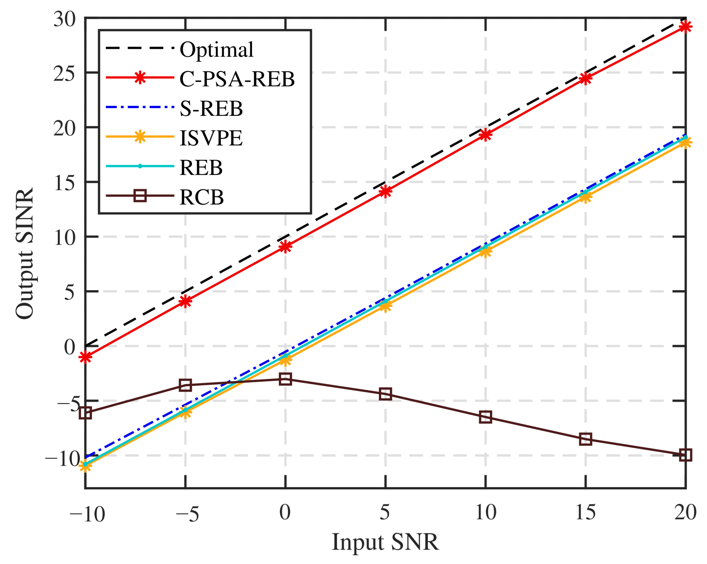
We simulated the change of the output SINR of each beamformer with the input SNR when the direction error occurred, and showed it in Figure 7. It can be seen that the proposed algorithm and S-REB have almost reached the optimal performance, because these two algorithms both use the signal subspace, therefore effectively improving the performance. The performance of REB and ISVPE is about 2 dB below the optimal SINR, but it is also better than the RCB algorithm based on SCM, especially with high SNR. It can be seen that as the SNR increases, the SINR of the RCB algorithm drops sharply, and the phenomenon of self-cancelation of the desired signal may appear.

In addition, we also show the impact of the number of snapshots on the performance in Figure 8. It can be seen that the SINR of ISVPE and RCB under the condition of small snapshots is as low as 15 dB and 4 dB, respectively. It may be because that the limited number of snapshots causes a large difference between the theoretical matrix and the estimated SCM. However, the other three beamformers, including the proposed one, are not sensitive to the number of snapshots because they use the reconstructed covariance matrix.

4.4. Performance Analysis with Local Scattering

In the fourth simulation, the influence of incoherent local scattering on the performance of the beamformer is studied. We assume that only the local scattering signal exists in the desired signal direction, i.e., the expected signal is several random signals around the assumed incident direction, and the SV of the scattered signal is time-varying [34]:

$${\tilde{s}}_0(k)={\mathbf{a}}_0{s}_0(k)+\sum _{p=1}^{N_p}\mathbf{a}\left({\theta }_p\right)s_p(k),$$

(33)

where $s_0$ is the direct signal, $N_p$ is the total number of local scattering signals, and $s_p$ is the incoherent local scattering signal. Similar to the direct signal, the local scattering signal is also generated from a Gaussian random process. $a_0$ is the SV corresponding to the direct signal, $\mathbf{a}({\theta }_p)$ is the SV of the local scattered signal, we assume that the incident angle of the scattered signal obeys a uniform distribution within $\left. [{13}^{\circ },{17}^{\circ }\right]$. $N_p$ is the number of local scattering signals, we set $N_p=4$ to be in this article.

Once the local scattering signal is considered, the rank of DSCM is no longer 1, i.e., the number of dominant eigenvalue of DSCM is more than 1. Therefore, in this case, we can use the dominant eigenvector to the largest eigenvalue of DSCM as the steering vector, and the weighting vector can also be written as the dominant eigenvector of ${\mathbf{R}}_{\mathrm{i}+\mathrm{n}}^{-1}{\mathbf{R}}_{\mathrm{s}}$.

We have simulated that when there are incoherent local scattering signals, the output SINR of each beamformer varies with the input SNR, and it is shown in the Figure 9. It can be seen that all reconstructed beamformers can perform well. By suppressing interference and noise, the algorithm proposed in this paper can be reach the optimal value just like S-REB. Due to the presence of local scattering signals, the RCB algorithm must deal with SV mismatches, which reduces the RCB’s performance to only 22 dB when input SNR is 20 dB. Then, we simulated the impact of the number of snapshots on performance and showed it in the Figure 10, similar to Figure 8, REB, S-REB and C-PSA-REB are all insensitive to the variation snapshot number, and the proposed C-PSA-REB can achieve 19.5 dB even in small snapshots.

Based on the theoretical analysis and numerical simulations, we summarize the employed techniques, the needed prior-knowledge, and the robustness in curvilinear trajectory of all tested beamformers in

Table 2. Comparison of the proposed beamformer and tested beamformers.

Beamformer	Employed Techniques	Needed Prior-Knowledge	Curvilinear Robustness
RCB [7]	Covariance matrix fitting + Convex optimization	Presumed SOI direction	No
REB [14]	Angular separation + Convex optimization	SOI angular sector	No
S-REB [17]	Subspace projection	Interference angular sector	No
ISVPE [32]	Interference SV and power estimation using RCB	DOAs of all incident signals	No
C-PSA-REB	Signal subspace fitting + Hybrid optimization	travel distance between measurements	Yes

.

4.5. Performance Analysis with Random Curvilinear Trajectory

This example, we investigate the beamformer performance in the case of random curvilinear trajectory and unknown DOAs of incident signals. We assume that the parameter ${\alpha }_m,m=1,2,\cdots ,M-1$ is uniformly distributed in $\left. [-{30}^{\circ },{30}^{\circ }\right]$, $\beta$ is uniformly distributed in $\left. [-{90}^{\circ },{90}^{\circ }\right]$, and direction errors are uniformly distributed in $[-4^{\circ },4^{\circ }]$.

Figure 11 demonstrates the performance of all tested beamformers with different input SNRs. With random curvilinear trajectory, the performance of REB, S-REB and ISVPE are all degraded severely, their output SINRs are generally lower than the optimal SINR around 13 dB. Moreover, RCB performs badly even when the SNR is low. By comparison to other tested beamformers, the proposed C-PSA-REB almost reaches the optimal SINR, which indicates the robustness.

Figure 12 shows the performance of all beamformers with different number of snapshots. Due to the severe deviation of trajectory, the performance of RCB is below −5 dB with different snapshots number. Other tested reconstruction-based beamformers are stabilized with different snapshots, and the proposed C-PSA-REB reaches nearly 20 dB, which obviously outperforms other tested beamformers.

5. Conclusions

In this paper, an adaptive beamformer is proposed for passive synthetic aperture with curvilinear trajectory by reconstructing INCM. Consider the trajectory of moving platform may be curvilinear, which will affect the performance of beamforming, the signal model of curvilinear trajectory is established. Then, a joint optimization problem is then constructed by applying the theory of subspace fitting, where the curvilinear trajectory parameters and the unknown DOAs are included. A hybrid optimization method was developed by combining the genetic algorithm and difference-based BFGS method, which can estimate a set of non-orthogonal bases for signal subspace with an acceptable computational complexity. Then, the DSCM is directly extracted from signal subspace using the set of non-orthogonal bases. By removing the SOI component from the SCM, we reconstruct a precise INCM without any known reference sources. In the end, numerical simulations demonstrate that the angle between the curved plane and the signal incident plane $\beta$ and the maximum deviation angle of trajectory ${\alpha }_{\max }$ are two key parameters that influence the performance of existing adaptive beamformers, and the proposed C-PSA-REB can perform robustly in different types of SV mismatches, even when the trajectory is severely curvilinear.