An Approach to Accuracy Assessment of ASTER Derived Mineral Maps

Abstract

An accuracy assessment of a classified thematic map is critical for the success of a remote sensing project. The identification and quantification of accuracy sources for classified mineral maps derived from satellite images enable confident decisions to be made for further exploration operations. Nineteen rock samples were collected from the different lithological units of the hydrothermally altered Kuh Panj Cu porphyry occurrence within the south-eastern part of Iran. SPECIM hyperspectral imaging was applied to the rock samples, followed by X-ray diffraction (XRD) analysis to compare the SPECIM mineral maps. The SPECIM results were then interpreted for mineralogy and compositional mapping extracted from the Advanced Spaceborne Thermal Emission and Reflection Radiometer (ASTER) images. The spectral angle mapper (SAM) and real value−area (RV−A) fractal methods were applied on SPECIM and ASTER images to interpret the mineralogy and derived classified map products. Two methods, including confusion matrix and one minus standard deviation over mean, were used to assess the accuracy of the classified SPECIM and ASTER derived mineral maps. Performing sensitivity studies were investigated, including the effect of spatially displacing ASTER mineral mapping and changing the SAM-derived threshold values on the accuracy of the ASTER mineral map. The sensitivity analyses demonstrated that selecting an optimum SAM-derived threshold value is more important than spatial displacement. Finally, accuracy sources were summarized in an accuracy budget table. The results demonstrated 89 and 88% accuracy for SPECIM and 88 and 92% accuracy for ASTER mineral maps via the confusion matrix and one minus standard deviation over mean methods, respectively. The accuracy budget helped to evaluate and compare all sources of accuracy with their accuracy values.

1. Introduction

The success of a remote sensing project depends on the accuracy of the classified output map. This can be related to the spatial and spectral resolution of the input data, disturbances in the remote sensing products, such as clouds, haze, shadow, the applied algorithm, and platform and sensor-related issues. Without accuracy assessment, the decision-making process for further operations, such as designing geophysical surveys, rock sampling, or locating exploratory drilling sites, cannot be done efficiently.

The spatial accuracy indicates the closeness of estimations and observations of remote sensing data to reality or a validated map [1,2]. The accuracy of a classified thematic map demonstrates the performance of the chosen method for mapping, and the accuracy of each class corresponds to the ground truth [3,4,5]. Many different methods, such as the error matrix, confusion matrix, and Kappa coefficient, are used to assess the accuracy of classified thematic maps. In most mineral exploration studies, the accuracy of mineral maps is derived from or based on, the remote sensing data [6,7,8,9,10,11]. However, they normally do not indicate what kind of accuracy sources were involved and how large these were. Therefore, in this research, we wanted to know: (a) the sources of accuracy, (b) how large they were, (c) how they contribute to the total accuracy, and (d) how can we prioritize them to improve the total accuracy?

This study aims to establish a procedure for identifying and quantifying the sources of accuracy for mineral maps derived from the Advanced Spaceborne Thermal Emission and Reflectance Radiometer (ASTER) data [12]. The mineral maps derived from ASTER images were compared with ground data through which the sources of accuracy were identified and quantified. This study helps geologists, earth scientists, and ASTER data users find accuracy sources playing a role in total accuracy and prioritize and improve them for mineral mapping projects. Any remote sensing product user could also use the accuracy budgeting methodology to assess the accuracy of different sources and prioritize and improve them, based on the project requirement(s).

2. Materials and Methods

2.1. Study Area and Geological Setting

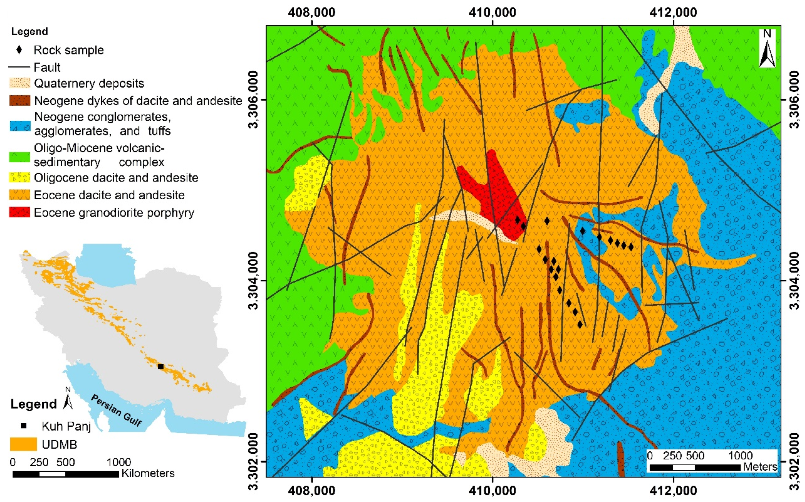
Our study was done on the Kuh Panj porphyry Cu mineralized occurrence area in Iran (Figure 1). Due to minimal semiarid vegetation coverage (shrubs, bushes, and occasional trees) and semidry weather with predominantly sunny days, this area is suitable for geological remote sensing investigations [13,14,15,16]. The geological history of the area involves the collision of the Arabian plate and the micro continental Iranian plate, which led to the subduction of the Neotethyan oceanic plate under the Iranian micro continental plate during the Paleocene to the Oligocene [17,18,19,20]. As a consequence, intensive calc-alkaline magmatic activities occurred that led to the formation of the Urumieh-Dokhtar Magmatic Belt (UDMB) in Iran (Figure 1) [21,22]. The Kuh Panj porphyry Cu occurrence is located within the south-eastern part of the UDMB. The hydrothermal alteration zones of potassic, argillic, phyllic, silicification, and propyllitic have been observed at the surface of the area [23,24,25].

2.2. Rock Sampling and Preparation

Nineteen outcrop rock samples were collected from two transects that intersect at the geometric center of the Kuh Panj area, covering dominant lithological and alteration units of the area (Figure 1; [23,25]). The rock sampling distance was approximately 200 m. Each rock sample had approximate dimensions of 7 × 5 × 4 cm. Although more rock samples would give us more accurate accuracy, we believe that the present number represents the composition of the rocks of the area.

The rock samples were cut into halves with a diamond sawn under water and dried in an oven for 24 h at 85 °C to eliminate water vapor and water in the rocks. Then, one-half of the samples were ground to powders (minus 63 micron) [26]. The powders were used for X-ray diffraction (XRD) analysis to interpret the dominant minerals and compare the SPECIM hyperspectral camera image results. The other halves of the samples were stored in case a measurement should be repeated.

2.3. SPECIM Data and SPECIM Mineral Mapping

The SPECIM platform [27] with OLES30 lens and with laboratory setup (30 cm measurement distance from the rock samples, 256 µm pixel size, and 98 mm image swath) was used to acquire hyperspectral images of the rock samples before cutting and drying. The SPECIM camera captures short-wave infrared (SWIR) images from a wavelength of 940 nm to 2540 nm with 6 nm spectral resolution. Scans were taken from the smoothest surface of the rock samples to reduce scattering effects.

Wavelength mapping in a pixel-by-pixel basis method [28,29,30,31] was used to collect endmembers from the whole surface of each rock sample. This method does not require prior knowledge about the mineral composition of a study area to choose endmembers. The endmembers were interpreted by matching the wavelength position and comparing the depth of absorption features of the endmembers with the spectral interpretation field manual, G-MEX [32]. The interpreted endmembers were used for mineral mapping via the spectral angle mapper (SAM) method [33]. The SAM method, as a supervised image classifier, maps the degree of similarity between unknown spectra and reference spectra [34]. The real value−area (RV−A) fractal method was applied on SAM rule images to select unbiased optimum threshold values for each mineral class [10,35,36]. The RV−A fractal method computes a power-law relationship between cumulative pixel areas and SAM estimated abundance pixel values above a certain threshold [37]. In this method, each break in the logarithmic plot shows a threshold value related to a mineral class. Each SAM-derived threshold value was mapped and interpreted, and then the most suitable threshold value for each mineral class was selected. The dominant SWIR active mineral of each rock was considered the representative mineral of that rock. The number of pixels for each mineral class over the total number of pixels for that rock ratio was used to compute and determine the dominant mineral of each rock sample.

2.4. Analytical Spectral Device

Since the SPECIM images only cover the SWIR range, an analytical spectral device (ASD) model 3, with a contact probe and with a high-resolution lamp setup [38], was used to interpret visible-near infrared (VNIR) range diagnostic minerals such as iron oxides within the samples. For each sample, eight points, at least, from different parts of the rock samples were selected to obtain spectra. Each spectrum of each rock sample was investigated to interpret VNIR active minerals.

2.5. XRD Setup

A Ni-filtered Cu Kα radiation tube with 1.54184 [A°] and a 2θ scanning of 0.01/s for 30 rounds were set on 30 kV voltage and 10 mA current for XRD measurements via a Bruker D2 Phaser [39]. The scanning step was from 6 to 80° (2θ). Two discriminators with the lower level at 0.18 mm and the upper level at 0.25 mm were used. We used a divergent slit of 0.06 mm, a detector slit of 8 mm, and a 1 mm knife to minimize scattering effects.

2.6. ASTER Data and ASTER Mineral Mapping

A cloud-free ASTER scene of surface reflectance and crosstalk-corrected SWIR-band imagery [40,41] acquired during summer (at 07:01′:15” of 15 July 2003) were downloaded from the EarthData website [42]. The SWIR images have a 30 m by 30 m pixel size. We have chosen ASTER imagery since it has six bands in the SWIR range and thereby allows us to discriminate different hydrothermal alteration minerals in phyllic, argillic, and propyllitic zones. Due to sparse vegetation cover, the low tilt angle of the sun, and high solar elevation, summer images have the highest accuracy for mineral mapping among all seasons [43].

The atmospheric and instrumental corrections, radiance conversion into surface reflectance, and the accuracy of corrected ASTER images have been described by Thome et al. (1999) and Iwasaki and Tanoka (2005) [40,41]. We decided to use atmospherically corrected, converted to surface reflectance, and crosstalk-corrected SWIR images of ASTER to avoid the effect of different atmospheric corrections on the accuracy of mineral maps. Although the surface reflectance and crosstalk-corrected SWIR images of ASTER have been corrected atmospherically, they are not fully geo-located. The same ASTER scene with the same acquisition date as the surface reflectance and crosstalk-corrected SWIR images, under the title of registered radiance at the sensor-precision terrain-corrected data, were downloaded from the EarthData website [42] for georeferencing. Some 584 control points were chosen within the whole ASTER scene and used to geo-locate surface reflectance, and crosstalk-corrected SWIR ASTER images with registered radiance at the sensor-precision terrain corrected. The control points included buildings, dams, a stadium, roads, benches of mines, and other recognizable constant phenomena in ASTER images. The root-mean-square (RMS) method was used to compute the spatial inaccuracy [1].

Depending on the processing level of the ASTER scene and its preprocessing methods, bands five and nine have different reflectance values than in situ measurement [24,43,44]. Band ratios 5/6 and 9/8 were suggested to correct bands five and nine reflectance values [44]. These ratios demonstrate the spectral reflectance differences between ASTER spectra with the resampled SPECIM to ASTER spectra. Band ratios 5/6 and 9/8 were applied on SPECIM and ASTER data. The differences between SPECIM and ASTER were added to bands five and nine of ASTER to correct their reflectance values.

The SWIR images of ASTER were used to extract endmembers by the spatial-spectral endmember extraction (SSEE) method [45,46]. The advantage of using image spectra for endmember selection is that the endmembers have the same atmospheric correction and the corresponding spectral and spatial resolution [34,43,47]. The endmembers were interpreted by comparing the overall shape, absorption features, and absorption depths with the resampled to ASTER SWIR bandpasses of SPECIM spectra derived from the rock samples. The average ASTER SWIR endmember spectral signatures of montmorillonite and montmorillonite+illite and illite were used to map minerals within the Kuh Panj area via spectral angle mapper (SAM). Montmorillonite and montmorillonite+illite with relatively low crystallinity illite were considered one group since they represent an argillic alteration zone; illite with relatively high crystallinity was considered another group as it represents the phyllic alteration zone. The RV−A fractal method was applied on each montmorillonite and montmorillonite+illite and illite SAM rule images to determine the unbiased optimum threshold values to create a mineral map. Based on our interpretation of the RV−A fractal method results for SAM rule images of ASTER, the radians threshold value of 0.07 was selected for illite, and montmorillonite and montmorillonite+illite.

For each mineral class, spectral statistics, including average and the average plus standard deviation and average minus standard deviation, to represent the likely highest and lowest spectral ranges were extracted from the total area mapped for the class. We used the statistical spectra to check the spectral variation within each mineral class and assess the mineral classification. The lower variation between the highest and the lowest standard deviation spectra shows the class’s pixel spectra closeness and shows the suitable mineral classification.

Although the study area contains a low vegetation coverage, it is a disturbing influence for mineral mapping. The normalized difference vegetation index (NDVI) was used to eliminate the vegetation effect in the spectra by applying a masking filter to exclude such vegetation cover [24]. The RV−A fractal method was used to select the optimum threshold value (1.43 radians).

2.7. Accuracy Computation of SPECIM Classified Mineral Maps

Two methods, the confusion matrix [48] and one minus standard deviation over mean [49,50,51], were used to compute the accuracy of the classified SPECIM mineral maps. Twenty random image spectra from each rock sample were chosen by using the random sampling tool of Environment for Visualizing Images (ENVI) software and interpreted [52]. The interpreted spectra were used to create confusion matrices and compute the accuracy of SPECIM mineral maps. Since we made the spectral interpretation manually by comparing it with the G-MEX manual, we knew the mineral composition of each rock sample. If we re-did the spectral identification, the results would be biased, and a false higher accuracy would be achieved. Therefore, the interpretation of the spectra of each rock sample was given to a colleague. However, this could include human error by misinterpretation of montmorillonite+illite spectra as illite and artificially decreasing the accuracy of SPECIM mineral maps. Therefore, one minus standard deviation over mean as a statistical method was used to compare the confusion matrix results. The mean and standard deviation values of each mineral class were extracted from that class’s area in the corresponding SAM rule image and used to compute the accuracy. Finally, the average of all classes was taken and represented as the SPECIM mineral map accuracy. A lower standard deviation value for a class demonstrates the closeness of spectra of that class to the mean spectrum. This closeness shows that the class’s pixel spectra are similar and indicate the same mineral composition within that class.

2.8. Agreement Comparison of SPECIM Interpretation with XRD Interpretation

In this study, ground truth information is defined as the agreement of SPECIM with XRD, as they are two different methods for analyzing the presence or absence of minerals. However, it might be possible to have a conflict in the presence or absence of a mineral composition due to fundamental differences in what they measure and geological processes, such as weathering and coating [53,54,55,56,57,58,59,60]. The percentage of disagreement should be included in the total accuracy budget. The confusion matrix and Kappa coefficient assessments were used to compare XRD with SPECIM.

2.9. Accuracy Computation of ASTER Classified Mineral Maps

The two methods of the confusion matrix and one minus standard deviation over mean were used to assess the accuracy of the mineral map derived from ASTER images. The SPECIM results (the dominant mineral of each rock sample) and the spatial location of the rock samples were used to make the confusion matrix and assess the accuracy of the classified ASTER mineral map. We used SPECIM versus ASTER rather than XRD versus ASTER because both SPECIM and ASTER are spectral-based measurements reflecting the surface of rocks within the area. As undertaken for the SPECIM imagery, each mineral class’s mean and standard deviation values were extracted from the area of that class in the corresponding SAM rule image. The mean and standard deviation values were used to compute the accuracy of each class via one minus standard deviation over the mean. The average accuracy value of mineral classes was computed and represented as the ASTER mineral map’s accuracy via one minus standard deviation over mean.

2.10. Sensitivity Analyses

Sensitivity analyses were undertaken on the classified ASTER mineral map to evaluate parameters that affect the accuracy of the mineral map derived from ASTER images. The parameters included SAM-derived threshold values and spatial displacement of the classified ASTER mineral map. Different SAM-derived threshold values change the occupied areas for each class and lead to different accuracy values via the confusion matrix. Spatial inaccuracy of ASTER images and the GPS field locations can also lead to inaccurate positioning accuracy estimates of the ASTER images in different directions and lead to different accuracy values via the confusion matrix.

2.10.1. Accuracy of ASTER Mineral Map with Different SAM Threshold Values

By selecting different radians threshold values from the SAM rule images, the mineral class boundary may change and lead to different accuracy values. An interval of 0.01 radians was added to and subtracted from the SAM optimum threshold values to compare the accuracy of ASTER mineral maps with higher and lower radians threshold values.

2.10.2. Accuracy of ASTER Mineral Map with Different Spatial Displacement

Compared to the orthorectified and georeferenced ASTER images (registered radiance at the sensor-precision terrain-corrected ASTER), the surface reflectance and crosstalk-corrected SWIR ASTER images have inherent spatial inaccuracies that were estimated by this study’s RMS computation. The used global positioning system (GPS) device, a Garmin 60CSx for recording the location of the rock samples, had a horizontal accuracy of ±10 m [61]. By considering these displacements together, the accuracy of the classified ASTER mineral map was assessed by artificially shifting the image registration by one pixel (e.g., 30 m) and two pixels (e.g., 60 m) to north, south, west, and east.

2.11. Accuracy Budgeting

Three parameters of accuracy contribution potential, accuracy improvement difficulty, and accuracy priority were defined for the accuracy budgeting [1,2,5]. The accuracy contribution potential was defined as the participation of an accuracy source in total accuracy and ranged from one as the lowest to three as the highest accuracy contribution. If by increasing a small amount in the accuracy of an accuracy source, the total accuracy value increases largely, then the accuracy value of that accuracy source participates a lot in the total accuracy, and the highest score of three should be dedicated to it; and if increasing the accuracy of an accuracy source does not lead to higher total accuracy then the lowest score of one should be dedicated to that accuracy source.

The accuracy improvement difficulty is defined as the capability of improving each accuracy source. It varies from one as very easy to five as very difficult to improve that item’s accuracy. Suppose by applying a method such as one of the atmospheric corrections, the accuracy value of an accuracy source significantly improves. In that case, the lowest score of one should be assigned to it. However, if the accuracy of an accuracy source is not improving by changing a method, the highest score of five should be given to that accuracy source.

Based on the accuracy contribution and the accuracy improvement difficulty, the accuracy sources are prioritized from one as the lowest to three as the highest priority. Suppose an accuracy source has the highest accuracy contribution score and the lowest accuracy improvement difficulty. In that case, that accuracy source gets the highest priority because it is easy to increase the total accuracy. If an accuracy source has the lowest accuracy contribution score and has the highest accuracy improvement difficulty, that accuracy source gets the lowest priority. Based on accuracy value, accuracy contribution, accuracy improvement difficulty, and priority of each accuracy item in this research, the accuracy table values are described. It should be mentioned that all these determinations are made by the remote sensing user’s experience and related literature and could be varied from user to user and project to project [5].

3. Results

3.1. SPECIM SWIR Mineral Maps and ASD VNIR Spectral Identification

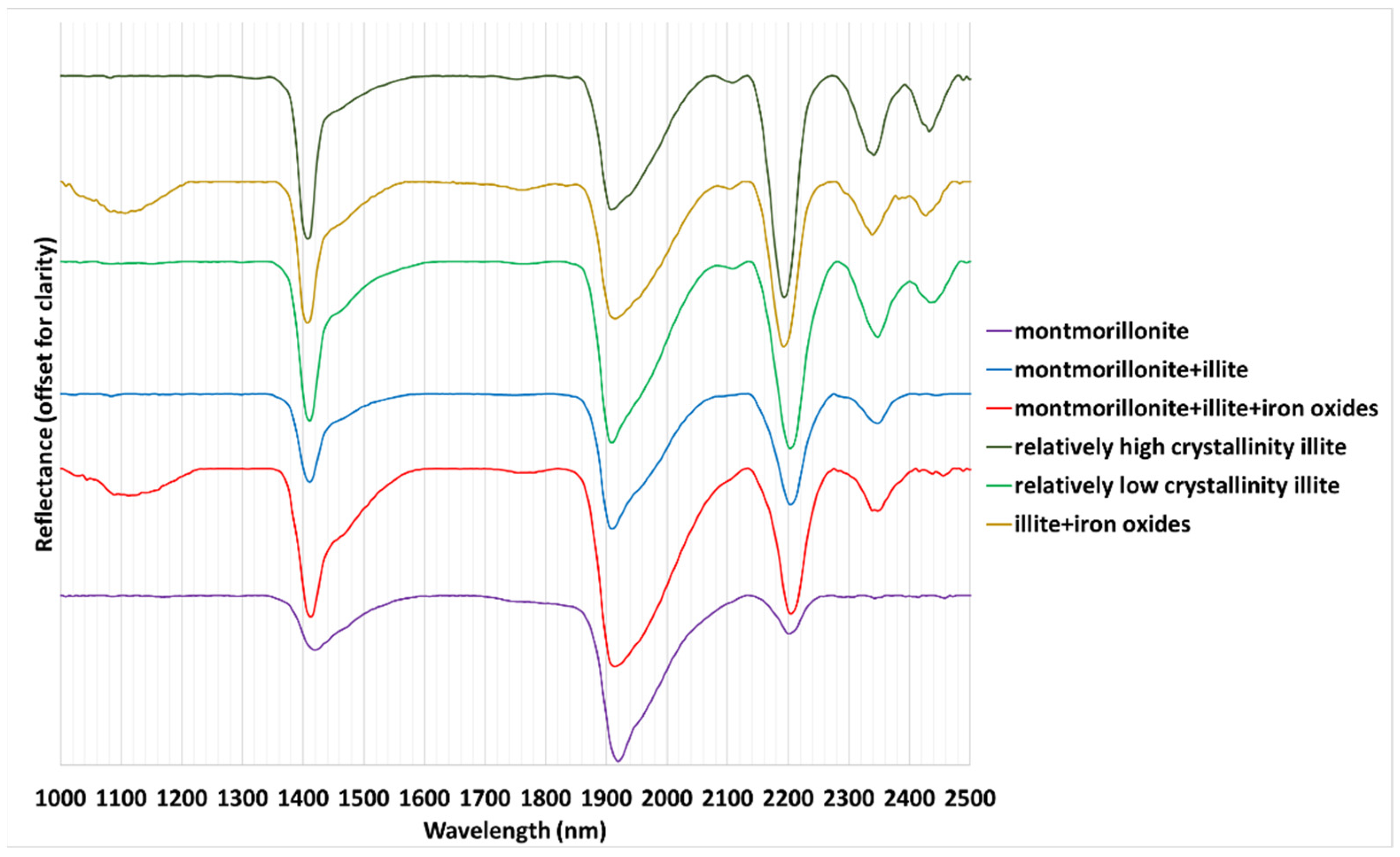
The SAM-derived SPECIM mineral maps demonstrated the presence of illite, montmorillonite, and their mixture, as well as iron oxides (Figure 2 and Figure 3). We have also identified iron oxides within our samples. In the SWIR range they are recognizable because of an absorption feature around 1100 nm. Based on the overall shape and wavelength of the absorption features of ASD spectra for the VNIR range, iron oxide minerals within the rock samples are interpreted as goethite and limonite [62,63].

Illite has crystallinity variations which are defined by dividing the depth of the aluminum hydroxyl absorption feature over the depth of the water absorption feature [64,65]. Two types of illite with relatively high crystallinity and relatively low crystallinity were interpreted within the samples. Samples that contain montmorillonite and montmorillonite+illite [66,67] have illite with relatively low crystallinity, while samples that contain only illite have relatively high crystallinity illites.

3.2. ASTER Mineral Map

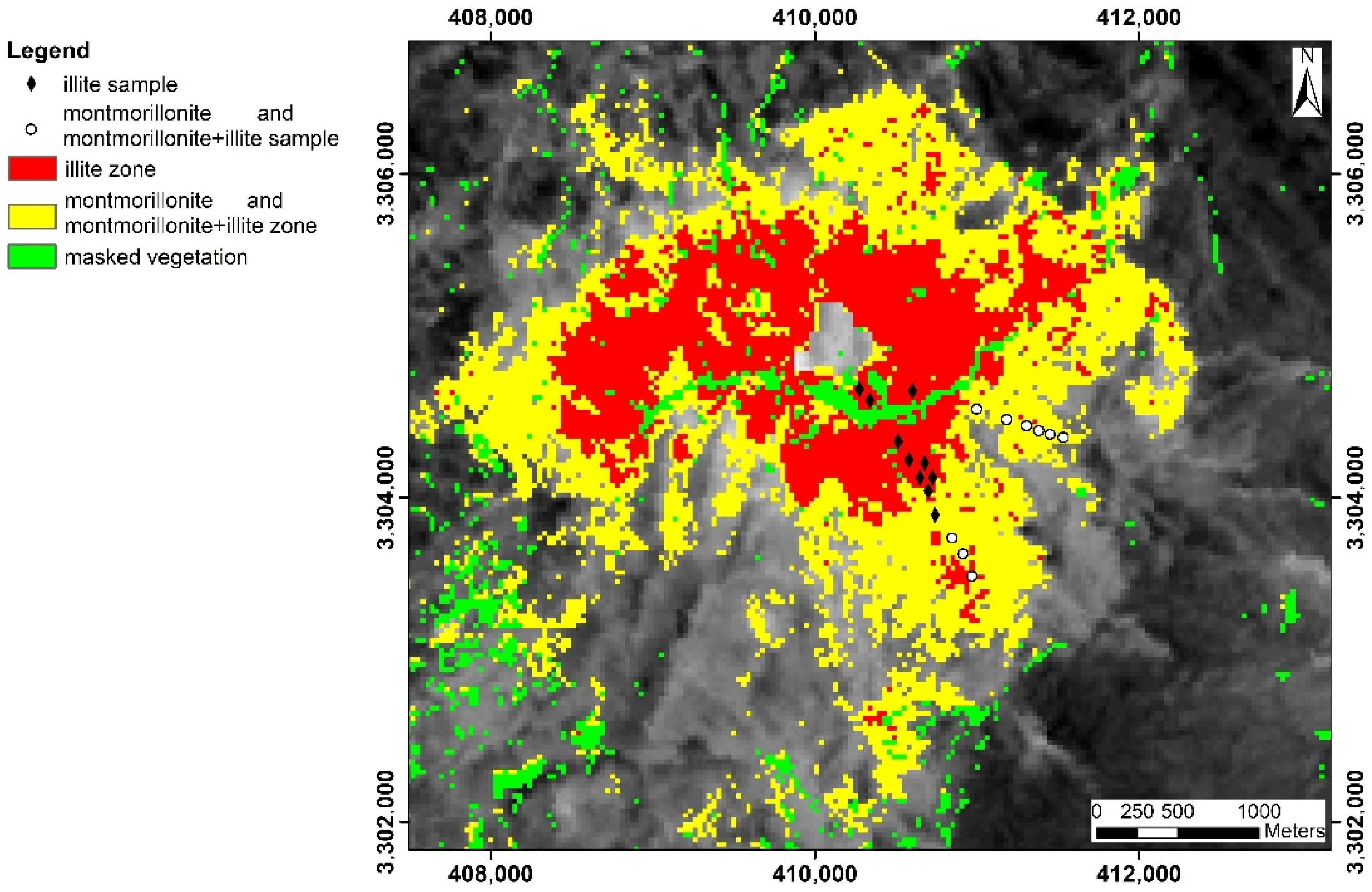
The SAM-processed ASTER mineral map of the study area demonstrated the donut-like spatial pattern for two mineral groups in which relatively high crystallinity illite was surrounded by montmorillonite and montmorillonite+illite with relatively low illite crystallinity (Figure 4). The ASTER spectrum of montmorillonite and montmorillonite+illite zone has shallower band eight absorption features than the illite spectrum of the illite zone. Montmorillonite and montmorillonite+illite spectra have a higher 5/6 band ratio value than the 7/6 band ratio value, while illite spectra have a higher 7/6 band ratio value than the 5/6 band ratio value.

The presence of illite-rich patches in the montmorillonite and montmorillonite+illite zone demonstrated the gradual increase of illite content in rocks. Khosravi (2007) [25] created the alteration map of the Kuh Panj area based on fieldwork and reported the presence of the potassic zone at the geometric center of the area as an outcrop. Our mineral mapping results via ASTER were consistent with the work of Pour et al. (2011 and 2012) and Zadeh et al. (2013) [13,14,15].

Standard deviations of 1.5% and 3% reflectance were observed for ASTER illite spectra within the illite zone and montmorillonite and montmorillonite+illite within the montmorillonite and montmorillonite+illite zone. These standard deviations show that the spectral variation within each zone was low, and from the spectral perspective, the mineral classification is accurate. The 3% variation for montmorillonite and montmorillonite+illite shows the different mixture ratios of montmorillonite with illite within the montmorillonite and montmorillonite+illite zone, which affect the reflectance value of bands five and eight of ASTER.

3.3. XRD Diffractogram Mineral Compositions

The XRD results demonstrated the presence of sheet silicates, quartz, and albite as the dominant minerals within the samples (Figure 5). Illite and muscovite share the same first 2θ peak at around 8.9°, quartz has sharp and large peaks at 21° and 27° 2θ, and albite has main peaks at around 14° and 28° 2θ [68,69,70]. Since muscovite was not confirmed and found in the SPECIM images, we conclude that the 8.9˚ 2θ peak belongs to illite. XRD results of Ayoobi and Tangestani (2017) [11] from the same area demonstrated the presence of montmorillonite. However, montmorillonite was absent within our XRD diffractograms (Figure 5). Montmorillonite has the first peak at around 6° to 8° 2θ [71,72]. This inconsistency between spectral-based measurements and XRD has been reported in some studies (e.g., [66]). The fundamental differences between the two measuring methods and geological processes explain the reason for this conflict. Electromagnetic radiation only can penetrate a few nanometers [58], and therefore, the SPECIM camera only measures the surface of the rock samples, which contain weathering and coating effects. However, the XRD device measures powders of the rock samples that contain fresh and nonweathered mineral compositions and penetrates particles with an approximate size of 63 microns.

The confusion matrix results of XRD versus SPECIM demonstrated 52% similarity (10 samples with the same mineral composition interpretation out of 19) in mineral composition interpretation. This similarity shows that both XRD and SPECIM confirm the presence of illite within the samples (those ten samples) as the dominant mineral. However, the presence of montmorillonite was not confirmed with XRD.

3.4. Accuracy of SPECIM Mineral Maps

The confusion matrix results for SPECIM mineral maps that were created with the randomly chosen and interpreted spectra demonstrated an average of 89% (±1%) accuracy, with an average Kappa coefficient of 0.78. The Kappa coefficient value showed that there is a high correlation existing between the interpreted SPECIM spectra and classified SPECIM mineral maps, which suggests the reliability of the classification of the SPECIM mineral maps [74]. The results of the one minus standard deviation over mean demonstrated an average of 88% (±2%) accuracy for each mineral class.

The results showed that the methods mentioned above for accuracy computation had close accuracy values to each other. However, the spectral similarity between illite and montmorillonite+illite was a possible source of inaccuracy for the SPECIM mineral maps. We believe that in SAM-derived mineral maps, both montmorillonite+illite and illite pixel spectra had close spectrum vectors in n-Dimensional space to each other. This closeness led to the smaller radians angles and a closer match between these two spectra.

The variation of water absorption depth at 1900 nm and variation of the aluminum hydroxyl absorption feature at around 2208 nm led to 0.02 higher SAM-derived radians angles (e.g., lower abundance) and higher standard deviation (±0.1). Consequently, a lower accuracy value was derived from one minus standard deviation over the mean method for montmorillonite, illite, and mixture together. The average accuracy value of classified SPECIM mineral maps demonstrated that these classified images are accurate and to be used for assessing the accuracy of mineral maps derived from ASTER images.

3.5. Accuracy of the ASTER Mineral Map

The confusion matrix result for the ASTER mineral map demonstrated an overall accuracy of 88% with a Kappa coefficient of 0.76. The Kappa coefficient showed a high correlation between SPECIM mineral maps and ASTER mineral map classes. The result of one minus standard deviation over mean demonstrated 92% (±1%) accuracy for the ASTER mineral map.

Similarities in the absorption features of the aluminum hydroxyl (2209 nm) and iron/magnesium hydroxyl (2330 nm) of montmorillonite+illite and illite led to the smaller radians angles and, therefore, a lower standard deviation, which led to higher accuracy via the one minus standard deviation over mean method. The accuracy value differences between the confusion matrix and one minus standard deviation over mean were less than 5%. The difference between accuracy values obtained from the confusion matrix and one minus standard deviation over the mean might be related to the limited number of samples used in this study. By increasing the number of ground samples, the confusion matrix accuracy might come closer to, or reaches, the accuracy of one minus standard deviation over mean. The accuracy values demonstrated that the ASTER mineral map represents sample (SPECIM) information with high accuracy and low uncertainty.

3.6. Sensitivity Analysis Results

3.6.1. Role of the SAM-Derived Threshold Value Selection on the Accuracy of ASTER Mineral Map

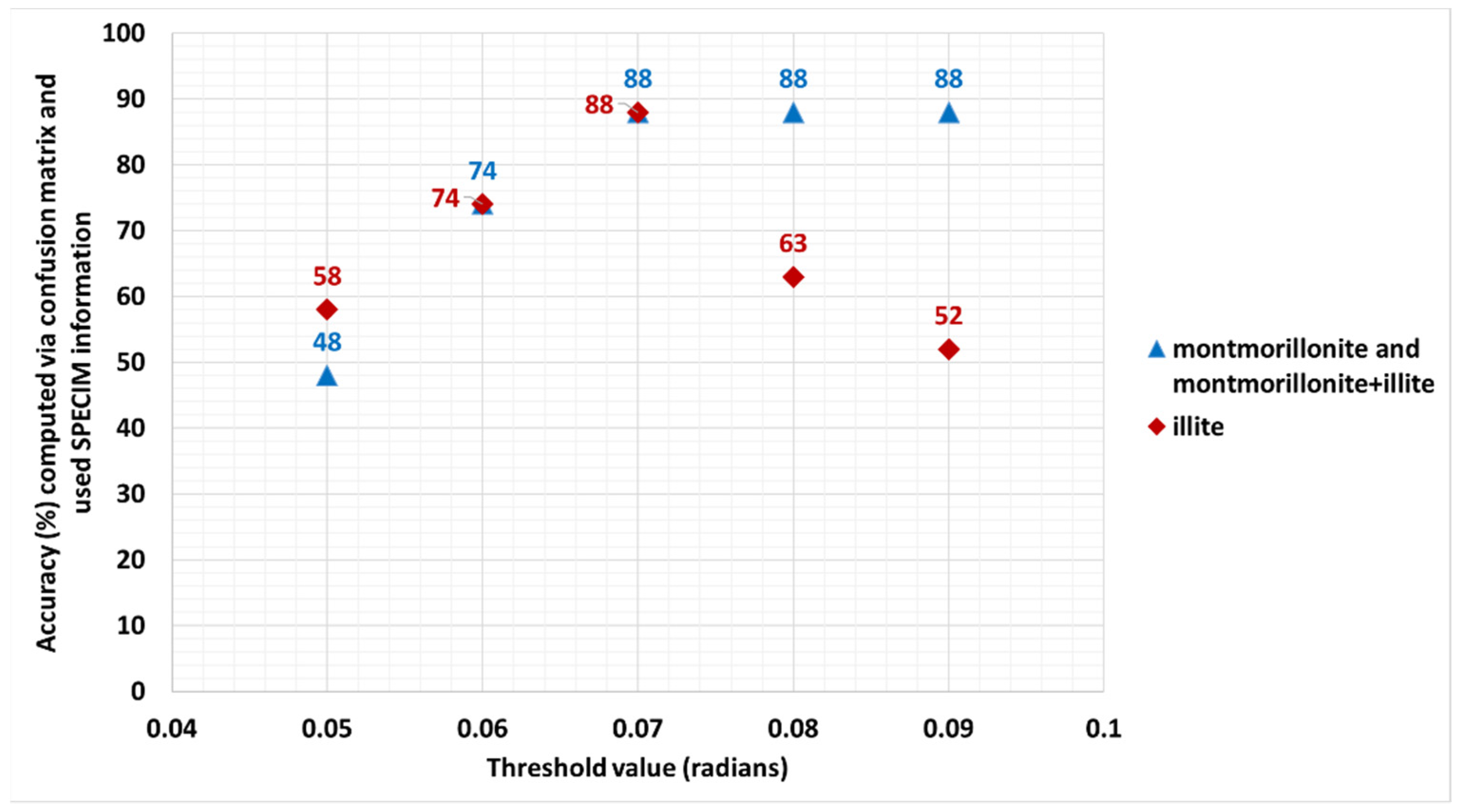
By increasing the threshold value of the SAM rule image of montmorillonite and montmorillonite+illite from 0.05 to 0.09 radians while the threshold value of illite was constant (0.07 radians), the accuracy of the ASTER mineral map increased from 48% for 0.05 radians threshold value to 88% for 0.07 and remained constant (88%) from 0.07 to 0.09 radians (Figure 6). By increasing the threshold value from 0.05 to 0.07 radians, the number of unclassified samples to classified samples dropped from ten samples to two and correctly classified, which led to the higher accuracy value.

By increasing the threshold value of illite from 0.05 to 0.07 radians while the threshold value of montmorillonite and montmorillonite+illite was constant (0.08 radians), the accuracy of the ASTER mineral map initially increased from 58 to 88%. However, the accuracy of the ASTER mineral map from the threshold values of 0.07 to 0.09 decreased from 88 to 52%. The number of incorrectly classified samples for the illite zone decreased from eight (for 0.05 radians) to one (for 0.07 radians) and then increased to all ten illite samples (for 0.09 radians) and led to the different accuracy values. The results show that a small (radians) threshold change for each mineral class had an impact on the accuracy of the ASTER mineral map. It should be mentioned that the accuracy of ASTER mineral maps derived from different SAM-derived threshold values were dependent on the location, density, and number of the rock samples. The results also showed that the RV−A fractal method is a suitable method for selecting optimum threshold values to obtain the highest classification accuracy.

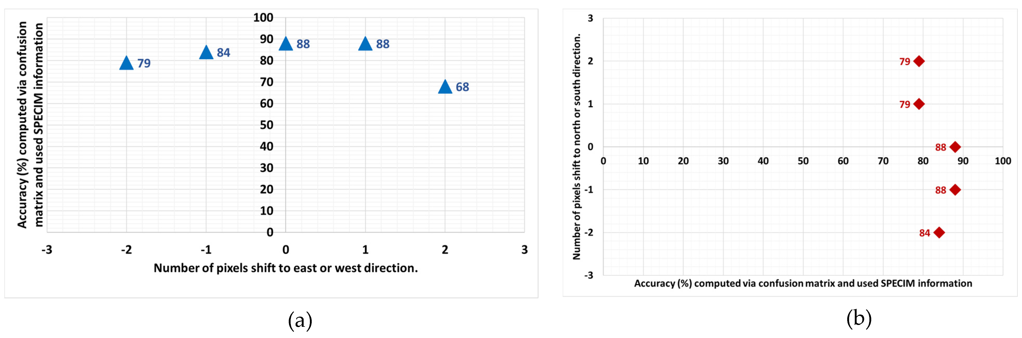
3.6.2. Role of Spatial Displacement on the Accuracy of ASTER Mineral Map

Some 584 control points were used for georeferencing the ASTER images, and the total RMS error for the whole ASTER scene was determined as 29 m (with a standard deviation of ± 15 m). The Garmin global position system (GPS) device had a horizontal accuracy of ± 10 m [61]. Therefore, the total spatial accuracy was about 39 ± 15 m (more than a 30 m by 30 m ASTER-SWIR image pixel size).

The results of shifting 1−2 pixel(s) to different directions are illustrated in Figure 7. They demonstrated that the accuracy of the ASTER mineral map reduced for all directions except for a pixel shift to the west and south in this study. The results showed that shifting 1−2 pixel(s) in the north-south direction had less ASTER mineral map accuracy variation (from 79 to 88%) than the west-east direction (from 68 to 88%). From west to center, the ASTER mineral map accuracy increased (from 79 to 88%) because the number of unclassified and misclassified samples decreased. However, the ASTER mineral map accuracy from the center to east decreased from 88 to 68%. From north to center, the accuracy of the ASTER mineral map increased from 79 to 88%, and then from center to the south, the accuracy of the ASTER mineral map decreased from 88 to 84% due to misclassification of the samples.

Comparing the spatial accuracy and threshold value effect on the accuracy of the ASTER mineral map demonstrated that threshold values had a higher impact on reducing the accuracy of the ASTER mineral map. By reducing the SAM-derived threshold values, the number of classified pixels to each mineral decreases; thus, more samples were misclassified and unclassified than the shifting location of each mineral zone.

4. Discussion

The accuracy budget is made up from different accuracy sources of SPECIM, and ASTER mineral maps, including accuracy values obtained from confusion matrix and one minus standard deviation over mean methods. The accuracy of the SPECIM mineral maps with both confusion matrix and one minus standard deviation over mean methods has the highest contribution potential score (3) to the total accuracy of the ASTER mineral map (

Table 1. Accuracy budget for the ASTER mineral map (accuracy contribution potential: 1 = low, 2 = medium, and 3 = high; accuracy control difficulty: 1 = very easy to 5 = very difficult; accuracy priority: 1 = low, 2 = medium, and 3 = high).

Imagery	Accuracy Source	Accuracy Contribution Potential	Accuracy Improvement Difficulty	Accuracy Priority	Accuracy Value (%)
SPECIM	Average mineral maps accuracy via confusion matrix	3	1	3	89
	Average mineral maps accuracy via one minus standard deviation over mean	3	1	3	88
	Agreement of interpreted minerals between SPECIM and XRD	3	2	3	52
ASTER	Mineral map accuracy via confusion matrix	3	1	3	88
	Average mineral map accuracy via one minus standard deviation over mean	3	2	3	92

). A SPECIM mineral map with low accuracy or incorrect classification could lower the accuracy and misclassify the ASTER mineral map. Therefore, the accuracy of the SPECIM mineral maps has the highest contribution potential score. Using the RV−A fractal method, optimum and unbiased threshold values were chosen easily for both SPECIM and ASTER mineral maps, so the lowest score of one is dedicated to improving the accuracy of SPECIM mineral maps. Based on the sensitivity analysis of Section 3.6 a small threshold value change (0.01 radians) led to a range of variations for the ASTER mineral map accuracy. Therefore, by selecting an optimum threshold value, the accuracy of the ASTER mineral map could increase easily. Since it was easy to improve the accuracy of the mineral maps, the lowest score of one was given. The average SPECIM mineral ma accuracy had the highest priority score due to its importance and the direct link to the ASTER mineral map.

XRD is an appropriate method that has been used for cross-validation of spectral-based mineral interpretation in many studies [e.g., 6–11]. The cross-validated samples decrease the mineral composition uncertainty of rock samples. Therefore, consistency between XRD and SPECIM results has the highest contribution potential score of three for total accuracy of ASTER and SPECIM mineral maps. Due to the fundamental differences between spectral measurements and XRD measurements and possible conflict results, it is not easy to use two methods to make cross-validation and ground truth information. Therefore, a score of two is given to the accuracy improvement of difficulty of XRD. An XRD measurement such as SPECIM has the highest priority to achieve the ground truth information; thus, the highest priority score of three should be dedicated to it.

The sensitivity analysis demonstrated that the accuracy of the ASTER mineral map varied from 52 to 88 percent by choosing different threshold values and displacing to different directions. Since the accuracies of all accuracy sources are accumulated in the accuracy of the ASTER mineral map, ASTER mineral maps have the highest accuracy contribution potential. The ASTER mineral map also has the highest priority to judge the overall accuracy of the work. This accuracy source is the least difficult to correct and improve the overall accuracy. Therefore, it has the highest priority score. The same as the SPECIM mineral maps, the highest ASTER mineral map’s accuracy was obtained using the RV−A fractal method that makes accuracy improvement the least difficult. Threshold values for ASTER and SPECIM mineral map classification showed the highest contribution to the mineral maps’ accuracy. Selecting the optimum threshold values was done easily with the RV−A fractal method, and it had the highest priority value since it directly affected the accuracy of mineral maps. Shifting pixels to different directions had a low contribution to the accuracy of the ASTER mineral map. It is easy to improve the accuracy of the ASTER mineral map by increasing the spatial accuracy by controlling a number of points of the images with already orthorectified and georeferenced images. Therefore, it has the lowest prioritizing accuracy.

5. Conclusions

A procedure to identify and quantify sources of accuracy for mineral mapping via the Advanced Spaceborne Thermal Emission and Reflectance Radiometer (ASTER) was established. The SPECIM hyperspectral images helped to interpret short-wave infrared (SWIR) active minerals within the rock samples. The X-ray diffraction (XRD) results were used to interpret non-SWIR active minerals within the samples and confirm the presence of sheet silicates. The real value−area (RV−A) fractal method was used to select the best threshold values for the classification of mineral maps to achieve the highest classification accuracy. One minus standard deviation over mean as an additional method confirmed the confusion matrix results for accuracy assessment. The selection of appropriate threshold values for mineral classification has more impact on the classified mineral map’s accuracy than spatial inaccuracy and displacement. Based on our study, we suggest that the threshold determination should have higher priority than georeferencing and spatial corrections in accuracy budgeting and assessment. The accuracy budget helped to achieve an overview of accuracy sources. The accuracy budget also encourages remote sensing users to consider, evaluate and compare all sources of accuracy in their project. The study was aimed at helping earth scientists who are using ASTER images to use accuracy budgeting for mineral mapping projects. In addition, the approach and methodology of this study can be used for more technically oriented scientists who want to do an accuracy assessment with hyper/multispectral images for different purposes.

The methodology developed in the current study can be applied elsewhere to assess and compare the accuracy values of classified ASTER mineral maps. It would be useful to examine other spaceborne/airborne hyperspectral/multispectral imagery to assess the accuracy of mineral maps within the same area and compare them with the ASTER-determined mineral map. Another mapping method could also be used to check the impact of different methods on the accuracy of ASTER mineral maps within the same area. We suggest collecting more samples, particularly more for each field site, to more confidently represent the 30 × 30 m ASTER pixels examined in the accuracy assessments. Further mineral composition measurements, such as low-angle XRD on fractioned clay powders, elutriation and thermogravimetric analysis (TGA) are highly recommended and suggested. The ASD spectra could be used to evaluate the inhomogeneity (mixed pixel) of the rock samples observed with the SPECIM data.

References

- Lunetta, R.; Congalton, R.; Fenstermarker, L.; Jensen, J.; McGwire, K.; Tinney, L. Remote sensing and geographic information system data integration: Error sources and research issues. Photogram. Eng. Remote Sens. 1991, 57, 677–687. [Google Scholar]
- Lunetta, R.S.; Lyon, J.G. Remote Sensing and GIS Accuracy Assessment; CRC Press: Boca Raton, FL, USA, 2004. [Google Scholar]
- Story, M.; Congalton, R.G. Accuracy assessment: A user’s perspective. Photogram. Eng. Remote Sens. 1986, 52, 397–399. [Google Scholar]
- Congalton, R.G. A review of assessing the accuracy of classifications of remotely sensed data. Remote Sens. Environ. 1991, 37, 35–46. [Google Scholar] [CrossRef]
- Congalton, R.G.; Green, K. Assessing the Accuracy of Remotely Sensed Data: Principles and Practices; CRC Press: Boca Raton, FL, USA, 2019. [Google Scholar]
- Honarmand, M.; Ranjbar, H.; Shahabpour, J. Application of spectral analysis in mapping hydrothermal alteration of the Northwestern Part of the Kerman Cenozoic Magmatic Arc, Iran. J. Sci. Islam. Repub. Iran 2011, 22, 221–238. [Google Scholar]
- Honarmand, M.; Ranjbar, H.; Shahabpour, J. Combined use of ASTER and ALI data for hydrothermal alteration mapping in the northwestern part of the Kerman magmatic arc, Iran. Int. J. Remote Sens. 2013, 34, 2023–2046. [Google Scholar] [CrossRef]
- Fereydooni, H.; Mojeddifar, S. A directed matched filtering algorithm (DMF) for discriminating hydrothermal alteration zones using the ASTER remote sensing data. Int. J. Appl. Earth Obs. Geoinf. 2017, 61, 1–13. [Google Scholar] [CrossRef]
- Mojeddifar, S.; Ranjbar, H.; Nezamabadipour, H. Adaptive neuro-fuzzy inference system application for hydrothermal al-teration mapping using ASTER data. J. Min. Environ. 2013, 4, 83–96. [Google Scholar]
- Shahriari, H.; Ranjbar, H.; Honarmand, M.; Carranza, E.J. Selection of Less Biased Threshold Angles for SAM Classification Using the Real Value-Area Fractal Technique. Resour. Geol. 2014, 64, 301–315. [Google Scholar] [CrossRef]
- Ayoobi, I.; Tangestani, M.H. Evaluating the effect of spatial subsetting on subpixel unmixing methodology applied to ASTER over a hydrothermally altered terrain. Int. J. Appl. Earth Obs. Geoinf. 2017, 62, 1–7. [Google Scholar] [CrossRef]
- Abrams, M.; Yamaguchi, Y. Twenty Years of ASTER Contributions to Lithologic Mapping and Mineral Exploration. Remote Sens. 2019, 11, 1394. [Google Scholar] [CrossRef]
- Pour, A.B.; Hashim, M. Identifying areas of high economic-potential copper mineralization using ASTER data in the Urumieh–Dokhtar Volcanic Belt, Iran. Adv. Space Res. 2012, 49, 753–769. [Google Scholar] [CrossRef]
- Pour, A.B.; Hashim, M. Identification of hydrothermal alteration minerals for exploring of porphyry copper deposit using ASTER data, SE Iran. J. Asian Earth Sci. 2011, 42, 1309–1323. [Google Scholar] [CrossRef]
- Zadeh, M.H.; Tangestani, M.H.; Roldán, F.V.; Yusta, I. Mineral Exploration and Alteration Zone Mapping Using Mixture Tuned Matched Filtering Approach on ASTER Data at the Central Part of Dehaj-Sarduiyeh Copper Belt, SE Iran. IEEE J. Sel. Top. Appl. Earth Obs. Remote Sens. 2013, 7, 284–289. [Google Scholar] [CrossRef]
- Zadeh, M.H.; Honarmand, M. A remote sensing-based discrimination of high- and low-potential mineralization for porphyry copper deposits; a case study from Dehaj–Sarduiyeh copper belt, SE Iran. Eur. J. Remote Sens. 2017, 50, 332–342. [Google Scholar] [CrossRef]
- Shafiei, B.; Haschke, M.; Shahabpour, J. Recycling of orogenic arc crust triggers porphyry Cu mineralization in Kerman Ce-nozoic arc rocks, south-eastern Iran. Miner. Depos. 2009, 44, 265. [Google Scholar] [CrossRef]
- Richards, J.P.; Sholeh, A. The Tethyan tectonic history and Cu-Au metallogeny of Iran. Tectonics and Metallogeny of the Tethyan Orogenic Belt. Society of Economic Geologists. Spec. Publ. 2016, 19, 193–212. [Google Scholar]
- Asadi, S.; Moore, F.; Zarasvandi, A. Discriminating productive and barren porphyry copper deposits in the south-eastern part of the central Iranian volcano-plutonic belt, Kerman region, Iran: A review. Earth Sci. Rev. 2014, 138, 25–46. [Google Scholar] [CrossRef]
- Asadi, S. Triggers for the generation of post–collisional porphyry Cu systems in the Kerman magmatic copper belt, Iran: New constraints from elemental and isotopic (Sr–Nd–Hf–O) data. Gondwana Res. 2018, 64, 97–121. [Google Scholar] [CrossRef]
- Ghorbani, M. Economic Geology of Iran; Springer: Berlin/Heidelberg, Germany, 2013; Volume 581. [Google Scholar]
- Dimitrijevic, M.D. Geology of Kerman region: Institute for geological and mining exploration and investigation, Beograd-Yugoslavia. Geol. Survey 1973, 52, 334. [Google Scholar]
- Nedimovic, R. Exploration for ore deposits in Kerman region, Beograd-Yugoslavia; Geological Survey of Iran (GSI): Tehran, Iran, 1973; 280p. [Google Scholar]
- Mars, J.C.; Rowan, L.C. Regional mapping of phyllic-and argillic-altered rocks in the Zagros magmatic arc, Iran, using Ad-vanced Spaceborne Thermal Emission and Reflection Radiometer (ASTER) data and logical operator algorithms. Geosphere 2006, 2, 161–186. [Google Scholar] [CrossRef]
- Khosravi, A. Statistical Geological and Alteration Map of Kuh Panj Copper Deposit; Exploration Department of National Iranian Copper Industries Company (NICICo): Sar Cheshmeh, Kerman, Iran, 2007. [Google Scholar]
- Maleki, S.; Karimi-Jashni, A. Effect of ball milling process on the structure of local clay and its adsorption performance for Ni(II) removal. Appl. Clay Sci. 2017, 137, 213–224. [Google Scholar] [CrossRef]
- SPECIM Spectral Imaging. Available online: https://www.specim.fi/products/swir/ (accessed on 23 April 2021).
- Bakker, W.; van Ruitenbeek, F.J.A.; van der Werff, H.M.A. Hyperspectral image mapping by automatic color coding of absorption features. In Proceedings of the 7th EARSEL Workshop of the Special Interest Group in Imaging Spectroscopy, Edinburgh, UK, 11–13 April 2011; pp. 56–57. [Google Scholar]
- van Ruitenbeek, F.J.; Bakker, W.H.; van der Werff, H.M.; Zegers, T.E.; Oosthoek, J.H.; Omer, Z.A.; Marsh, S.H.; van der Meer, F.D. Mapping the wavelength position of deepest absorption features to explore mineral diversity in hyperspectral images. Planet. Space Sci. 2014, 101, 108–117. [Google Scholar] [CrossRef]
- van der Meer, F.; Kopačková, V.; Koucká, L.; van der Werff, H.M.; van Ruitenbeek, F.J.A.; Bakker, W.H. Wavelength feature mapping as a proxy to mineral chemistry for investigating geologic systems: An example from the Rodalquilar epithermal system. Int. J. Appl. Earth Obs. Geoinf. 2018, 64, 237–248. [Google Scholar] [CrossRef]
- Hecker, C.; van Ruitenbeek, F.J.A.; Bakker, W.H.; Fagbohun, B.J.; Riley, D.; van der Werff, H.M.; van der Meer, F.D. Mapping the wavelength position of mineral features in hyperspectral thermal infrared data. Int. J. Appl. Earth Obs. Geoinf. 2019, 79, 133–140. [Google Scholar] [CrossRef]
- Pontual, S.; Merry, N.; Gamson, P. Spectral interpretation field manual, G-MEX. In Spectral Analysis Guides for Mineral Exploration; AusSpec International Pty. Ltd.: Victoria, Australia, 1997; Volume 1. [Google Scholar]
- Kruse, F.; Lefkoff, A.; Boardman, J.; Heidebrecht, K.; Shapiro, A.; Barloon, P.; Goetz, A. The spectral image processing system (SIPS)—interactive visualization and analysis of imaging spectrometer data. Remote Sens. Environ. 1993, 44, 145–163. [Google Scholar] [CrossRef]
- Hecker, C.; van der Meijde, M.; van der Werff, H.; van der Meer, F.D. Assessing the influence of reference spectra on synthetic SAM classification results. IEEE Trans. Geosci. Remote Sens. 2008, 46, 4162–4172. [Google Scholar] [CrossRef]
- Shahriari, H.; Ranjbar, H.; Honarmand, M. Image segmentation for hydrothermal alteration mapping using PCA and con-centration–area fractal model. Nat. Resour. Res. 2013, 22, 191–206. [Google Scholar] [CrossRef]
- Chen, Q.; Zhao, Z.; Jiang, Q.; Zhou, J.-X.; Tian, Y.; Zeng, S.; Wang, J. Detecting subtle alteration information from ASTER data using a multifractal-based method: A case study from Wuliang Mountain, SW China. Ore Geol. Rev. 2019, 115, 103182. [Google Scholar] [CrossRef]
- Cheng, Q.; Li, Q. A fractal concentration–area method for assigning a color palette for image representation. Comput. Geosci. 2002, 28, 567–575. [Google Scholar] [CrossRef]
- Malvern Panalytical. Available online: https://www.malvernpanalytical.com/en/products/product-range/asd-range (accessed on 23 April 2021).
- Bruker X-ray Diffraction, D2 Phaser. Available online: https://www.bruker.com/products/x-ray-diffraction-and-elemental-analysis/x-ray-diffraction/d2-phaser.html (accessed on 23 April 2021).
- Thome, K.; Biggar, S.; Takashima, T. Algorithm Theoretical Basis Document for ASTER Level 2B1—Surface Radiance and ASTER Level 2B5—Surface Reflectance 1999. p. 45. Available online: http://eospso.gsfc.nasa.gov/index.php (accessed on 23 June 2021).
- Iwasaki, A.; Tonooka, H. Validation of a crosstalk correction algorithm for ASTER/SWIR. IEEE Trans. Geosci. Remote Sens. 2005, 43, 2747–2751. [Google Scholar] [CrossRef]
- Earthdata. Available online: https://earthdata.nasa.gov/ (accessed on 23 April 2021).
- Shahriari, H.; Honarmand, M.; Ranjbar, H. Comparison of multi-temporal ASTER images for hydrothermal alteration mapping using a fractal-aided SAM method. Int. J. Remote Sens. 2015, 36, 1271–1289. [Google Scholar] [CrossRef]
- Mars, J.C.; Rowan, L.C. Spectral assessment of new ASTER SWIR surface reflectance data products for spectroscopic mapping of rocks and minerals. Remote Sens. Environ. 2010, 114, 2011–2025. [Google Scholar] [CrossRef]
- Rogge, D.; Rivard, B.; Zhang, J.; Sanchez, A.; Harris, J.; Feng, J. Integration of spatial–spectral information for the improved extraction of endmembers. Remote Sens. Environ. 2007, 110, 287–303. [Google Scholar] [CrossRef]
- Gil, L.I.J.; Sanchez, S.; Martan, G.; Plaza, J.; Plaza, A.J. Parallel Implementation of Spatial–Spectral Endmember Extraction on Graphic Processing Units. IEEE J. Sel. Top. Appl. Earth Obs. Remote Sens. 2017, 10, 1247–1255. [Google Scholar] [CrossRef]
- Honarmand, M.; Ranjbar, H.; Shahriari, H.; Naseri, F. Evaluating the effect of using different reference spectra on SAM clas-sification results: An implication for hydrothermal alteration mapping. J. Min. Environ. 2018, 9, 981–997. [Google Scholar]
- Congalton, R.G.; Oderwald, R.G.; Mead, R.A. Assessing Landsat classification accuracy using discrete multivariate analysis statistical techniques. Photogramm. Eng. Remote Sens. 1983, 49, 1671–1678. [Google Scholar]
- Steel, R.G.; Torrie, J.H. Principles and Procedures of Statistics; McGraw-Hill: New York, NY, USA, 1960. [Google Scholar]
- Cormack, R.M.; Bliss, C.I. Statistics in Biology: Statistical Methods for Research in the Natural Sciences. J. R. Stat. Soc. Ser. A (General) 1968, 131, 610. [Google Scholar] [CrossRef]
- Overman, A.R.; Scholtz, R.V., III. Mathematical Models of Crop Growth and Yield; CRC Press: Boca Raton, FL, USA, 2002. [Google Scholar]
- ENVI-L3Harris Geospatial Solutions. Available online: https://www.l3harrisgeospatial.com/Software-Technology/ENVI (accessed on 23 April 2021).
- Beavis, F.C.; Roberts, F.I.; Minskaya, L. Engineering aspects of weathering of low grade metapelites in an arid climatic zone. Q. J. Eng. Geol. Hydrogeol. 1982, 15, 29–45. [Google Scholar] [CrossRef]
- Akpokodje, E.G. The mineralogical relationship between some arid zone soils and their underlying bedrocks at Fowlers Gap Station. New South Wales, Australia. J. Proc. R. Soc. N. S. W. 1987, 120, 90–99. [Google Scholar]
- Dragovich, D. A preliminary electron probe study of microchemical variations in desert varnish in Western New South Wales, Australia. Earth Surf. Process. Landforms 1988, 13, 259–270. [Google Scholar] [CrossRef]
- Potter, R.M.; Rossman, G.R. Desert Varnish: The Importance of Clay Minerals. Science 1977, 196, 1446–1448. [Google Scholar] [CrossRef] [PubMed]
- Lyon, R.J.P. Effects of Weathering, Desert-varnish, Etc. On Spectral Signatures of Mafic, Ultramafic and Felsic Rocks, Leonorawest Australia. In 10th Annual International Symposium on Geoscience and Remote Sensing; IEEE: Piscataway, NJ, USA, 1990; pp. 1719–1722. [Google Scholar]
- Elachi, C. Spaceborne Radar Remote Sensing: Applications and Techniques; IEEE: Piscataway, NJ, USA, 1988. [Google Scholar]
- Spatz, D.M.; Taranik, J.V.; Hsu, L.C. Desert varnish on volcanic rocks of the Basin and Range province- Composition, morphology, distribution, origin and influence on Landsat imagery. In Proceedings of the 21st International Symposium on Remote Sensing of Environment, Ann Arbor, MI, USA, January 1987; pp. 843–852. [Google Scholar]
- Rivard, B.; Arvidson, R.E.; Duncan, I.J.; Sultan, M.; El Kaliouby, B. Varnish, sediment, and rock controls on spectral reflectance of outcrops in arid regions. Geology 1992, 20, 295. [Google Scholar] [CrossRef]
- GPSMAP, Garmin. 60CSx User’s Manual 2007. Available online: https://buy.garmin.com/nl-NL/NL/p/310 (accessed on 23 April 2021).
- Hunt, G.R. Spectral signatures of particulate minerals in the visible and near infrared. Geophysics 1977, 42, 501–513. [Google Scholar] [CrossRef]
- Clark, R.N.; King, T.V.V.; Klejwa, M.; Swayze, G.A.; Vergo, N. High spectral resolution reflectance spectroscopy of minerals. J. Geophys. Res. Space Phys. 1990, 95, 12653–12680. [Google Scholar] [CrossRef]
- Dalm, M.; Buxton, M.W.N.; Van Ruitenbeek, F.J.A. Discriminating ore and waste in a porphyry copper deposit using short-wavelength infrared (SWIR) hyperspectral imagery. Miner. Eng. 2017, 105, 10–18. [Google Scholar] [CrossRef]
- Dalm, M.; Buxton, M.W.; van Ruitenbeek, F.J.; Voncken, J.H. Application of near-infrared spectroscopy to sensor based sorting of a porphyry copper ore. Miner. Eng. 2014, 58, 7–16. [Google Scholar] [CrossRef]
- Simpson, M.P.; Rae, A.J. Short-wave Infrared (SWIR) reflectance spectrometric characterisation of clays from geothermal systems of the Taupo volcanic zone, New 737 Zealand. Geothermics 2018, 73, 74–90. [Google Scholar] [CrossRef]
- Jeong, Y.; Yu, J.; Wang, L.; Shin, J.H. Spectral Responses of As and Pb Contamination in Tailings of a Hydrothermal Ore Deposit: A Case Study of Samgwang Mine, South Korea. Remote Sens. 2018, 10, 1830. [Google Scholar] [CrossRef]
- Pei, Y.; Chen, P.Y. Table of Key Lines in X-ray Powder Diffraction Patterns of Minerals in Clays and Associated Rocks; Geological Survey Occasional report; Department of Natural Resources: Bloomington, IN, USA, 1977. [Google Scholar]
- McAlister, J.; Smith, B. A Rapid Preparation Technique for X-Ray Diffraction Analysis of Clay Minerals in Weathered Rock Materials. Microchem. J. 1995, 52, 53–61. [Google Scholar] [CrossRef]
- Chipera, S.J.; Bish, D.L. Baseline studies of the clay minerals society source clays: Powder X-ray diffraction analyses. Clays Clay Miner. 2001, 49, 398–409. [Google Scholar] [CrossRef]
- Castellini, E.; Berthold, C.; Malferrari, D.; Bernini, F. Sodium hexametaphosphate interaction with 2:1 clay minerals illite and montmorillonite. Appl. Clay Sci. 2013, 83–84, 162–170. [Google Scholar] [CrossRef]
- Szczerba, M.; Kłapyta, Z.; Kalinichev, A. Ethylene glycol intercalation in smectites. Molecular dynamics simulation studies. Appl. Clay Sci. 2014, 91–92, 87–97. [Google Scholar] [CrossRef][Green Version]
- Whitney, D.L.; Evans, B.W. Abbreviations for names of rock-forming minerals. Am. Miner. 2009, 95, 185–187. [Google Scholar] [CrossRef]
- McHugh, M.L. Interrater reliability: The kappa statistic. Biochem. Med. 2012, 22, 276–282. [Google Scholar] [CrossRef]