Abstract
The aerosol optical depth (AOD), retrieved by satellites, has been widely used to estimate ground-level PM2.5 mass concentrations, due to its advantage of large-scale spatial continuity. However, it is difficult to obtain urban-scale pollution patterns from the coarse resolution retrieval results (e.g., 1 km, 3 km, or 10 km) at present, and little research has been conducted on PM2.5 mass concentration retrieval from high resolution remote sensing data. In this study, a physical model is proposed based on Mie scattering theory to evaluate the PM2.5 mass concentrations by using Landsat8 Operational Land Imager (OLI) images. First, the Second Simulation of the Satellite Signal in the Solar Spectrum (6S) model (which can simulate the transmission process of solar radiation in the Earth-atmosphere system and calculate the radiance at the top of the atmosphere) is used to build a lookup table to retrieve the AOD of the coast and blue bands based on the improved deep blue (DB) method. Then, the Angstrom formula is used to obtain the AOD of the green and red bands. Second, the dry near-surface AOD of four bands (coast, blue, green, red) is obtained through vertical correction and humidity correction. Third, aerosol particles are divided into four types based on the standard radiation atmosphere (SRA) model, and the optical properties of different aerosol types are analyzed to derive the volume distribution of aerosol particles. Finally, the relationship between the dry near-surface AOD of each band and the volume distribution of four aerosol particles is correlated, based on Mie scattering theory, and a physical model is established between the AOD and PM2.5 mass concentrations. Then, the distribution of PM2.5 mass concentrations is obtained. The retrieval results show that the distribution of AOD and PM2.5 at the urban scale in detail. The AOD results show that a reasonable relationship with a correlation coefficient (R2) of 0.66 and root mean square error (RMSE) of 0.1037 between Landsat8 OLI AOD and MODO4 DB AOD at 550 nm. The PM2.5 retrieval results are compared with the PM2.5 values measured by ground monitoring stations. The RMSEs for a certain day in different years, including 2017, 2018, 2019, and 2020, are 11.9470 μg/m³, 11.9787 μg/m³, 7.4217 μg/m³, and 5.4723 μg/m³, respectively. The total RMSE is 10.0224 μg/m³. The ultrahigh resolution PM2.5 results can provide pollution details at the urban scale and support better decisions on urban atmospheric environmental governance.
1. Introduction
Aerosol particulate matter with an aerodynamic diameter smaller than 2.5 μm is called PM2.5, which can enter the lungs and cause various cardiovascular and respiratory diseases [1,2,3,4]. Since the beginning of the 21st century, the PM2.5 pollution problem has worsened over China; therefore, PM2.5 monitoring and governance have become particularly significant [5,6]. Currently, monitoring PM2.5 in large areas and multiple phases is difficult to achieve, due to the sparse and spatially discontinuous distribution of PM2.5 data from traditional ground sites, as well as limited labor, material, and financial resources. Remote sensing satellite monitoring can overcome these shortcomings and compensate for problems related to the spatial scale [7,8]. The satellite retrieval of aerosol can also provide aerosol optical properties, such as the aerosol optical depth (AOD), wavelength index, and turbidity coefficient [9,10,11,12]. However, the retrieval of PM2.5 mass concentrations still faces many challenges. For example, near-surface PM2.5 refers to the mass concentration of particulate matter under dry conditions, and AOD retrieved by remote sensing represents the extinction of the entire layer of atmospheric aerosol particles. The relationship between the AOD and PM2.5 mass concentrations is affected by many factors (such as the characteristics and distribution of PM2.5 [13], atmospheric vertical profile, relative humidity, and meteorological parameters [14,15]). By considering these influencing factors, the relationship between the AOD and PM2.5 mass concentrations can be determined [16].
Early research assumed that the relationship between AOD and PM2.5 mass concentrations was unknown. Linear or nonlinear regression was used to express their correlation, and various statistical relationships between AOD and PM2.5 mass concentrations were directly established [17,18,19,20]. However, these statistical models face many problems when they are applied to different areas and time periods, and it is difficult to present a universal relationship between AOD and PM2.5 mass concentrations. Subsequent studies included some meteorological factors (such as relative humidity (RH), wind speed (WS), temperature (TEMP), and planetary boundary layer height (PBLH)) in these models to correct the AOD and established empirical relationships between AOD and PM2.5 mass concentrations [21,22,23]. Although the accuracy of these models has been improved, there is still a lack of research on the optical characteristics of PM2.5, and the models have no clear physical significance. More recently, some related studies have used neural networks and machine learning to obtain more accurate regression relationships than earlier linear and nonlinear models [24,25]. Furthermore, atmospheric chemistry models have been used as another approach to solve the AOD-PM2.5 mass concentration conversion [26,27,28]. Although good results have been obtained, this approach is largely affected by the simulation scale, driving factors, and chemical mechanisms and is not applicable in extreme conditions (e.g., heavy pollution events). Zhang et al. [29] proposed a physical model by simulating the relationship between the fine particle column volume () and fine mode fraction (FMF) of different aerosol types and discovered that the and FMF have good regularity, finally establishing an AOD-PM2.5 mass concentration model and obtaining the near-surface PM2.5 mass concentrations. Obtaining the fine mode parameter in different ways (MOIDS, AERONET, PARASOL, etc.) leads to a lack of conformity and insufficient stability in the parameter, affecting retrieval accuracy. In addition, different satellite AOD products, mainly including the Moderate Resolution Imaging Spectroradiometer (MODIS) [30,31], Visible Infrared Imaging Radiometer Suite (VIIRS) [32,33], and Multiangle Imaging Spectro Radiometer (MISR) [34], were adopted to estimate PM2.5 mass concentrations in previous studies. However, the AOD data of these satellite products have different nominal spatial resolutions (MODIS (3 km or 10 km), VIIRS (6 km), MISR (17.6 km)); as a result, the resolutions of PM2.5 mass concentrations were too coarse to satisfy urban scale exposure requirements. Therefore, high resolution sensors (Landsat series, Gaofen series, etc.) have broad application prospects in evaluating PM2.5 mass concentrations.
Aiming to address the above problems, this paper proposes a new physically-based method to retrieve ultrahigh resolution PM2.5 mass concentrations from multiband AOD. In our proposed method, first, high-resolution AOD (30 m × 30 m) over the Pearl River Delta (PRD) region was retrieved from Landsat8 Operational Land Imager (OLI) coast and blue spectral band data using the improved deep blue (DB) method [11], and then the Angstrom formula was used to obtain the AOD of the green and red bands. In the process, both the original Landsat8 OLI data and the surface reflectance data were from the United States Geological Survey (USGS) website. An aerosol model was determined by statistical analysis of long-term ground monitoring CE318 data. Second, the dry near-surface AOD of each band was obtained from RH and PBLH data by humidity correction and vertical correction. These data were from the China Environmental Monitoring Station (CEMS) and European Centre for Medium-Range Weather Forecasts (ECMWF). Third, to avoid directly obtaining FMF, the aerosol particles were divided into four types based on the standard radiation atmosphere (SRA) model, and the optical properties of different aerosol types were analyzed to derive the volume distribution of aerosol particles. Then, the relationship between the dry near-surface AOD of each band and the volume distribution of four aerosol particles was correlated based on Mie scattering theory, and a physical model was established between AOD and PM2.5 mass concentrations. To verify our proposed method, the distribution of AOD and PM2.5 is presented at the urban scale. The AOD results were compared with MODO4 DB AOD products. The PM2.5 results were verified by ground monitoring sites. Finally, the performance and limitations of the model are also discussed.
This paper is organized as follows: Section 2 introduces materials and related methods; Section 3 mainly shows the distribution results of AOD and PM2.5 mass concentrations; Section 4 discusses some advantages and limitations of this method by comparing it with other studies; and Section 5 is the conclusion of this paper.
2. Materials and Methods
2.1. Study Area and Datasets
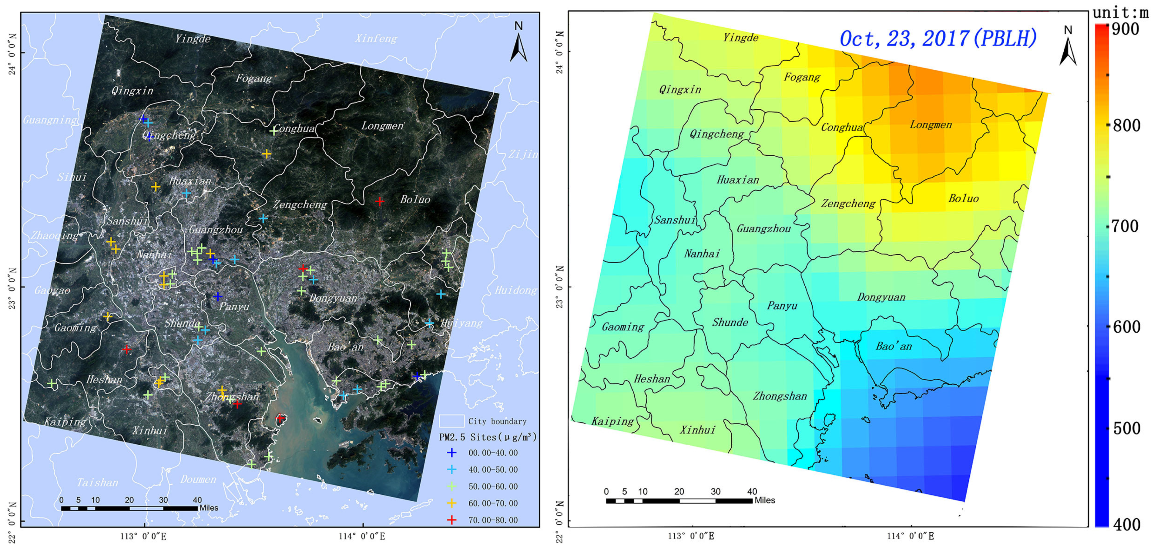
The study area in this paper is part of the PRD, located in Guangdong Province of China, bordering the South China Sea (Figure 1 Left). The longitude of the study area is between 112°23′ and 114°54′, and the latitude is between 21°49′ and 24°09′. With the development of industrialization in the PRD over recent decades, regional air pollution has gradually increased and spread [35,36]. Therefore, remote sensing retrieval of PM2.5 mass concentrations over the PRD region is significant.
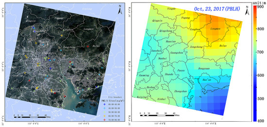
Figure 1.
(Left): The study area (part of the PRD) and the distribution of PM2.5 sites (in gradient colors corresponding to the annual average PM2.5 mass concentration on 23 October 2017); (Right): PBLH data in the study area (using the data on 23 October 2017 as a display).
As shown in Table 1, this paper used the following data: (a) Landsat8 OLI image data and reflectance data from the USGS (https://glovis.usgs.gov/, accessed on 9 October 2020), which have 11 bands (the spatial resolution of band 1–7, 9–11 is 30 m, and band 8 is a panchromatic band with 15m resolution) and a round trip period of about 16 days. The surface reflectance data was from atmospherically-corrected datasets from Landsat8 OLI sensor. Since only the visible bands of Landsat8 OLI were used to retrieve AOD in this paper, Table 2 mainly displays the detailed characteristics of these bands. All Landsat8 OLI image data have been preprocessed before beginning the AOD retrieval process. The preprocesses include geometric correction and radiometric calibration. The accuracy of the geometric correction is maintained at 1~2 pixels. We selected a certain day of the image with better data quality as experimental data in different years (including 2017–2020); (b) Hourly PM2.5 site data and RH data from the weather stations of CEMS (http://data.cma.cn/, accessed on 25 October 2020). The distribution of weather stations in the study area is shown in Figure 1. The stations can provide average measured PM2.5 and RH values within one hour; thus, we select the hourly average PM2.5 values close to imaging time as validation data. RH data is mainly used to study the moisture absorption characteristics of aerosol particles, which helps to obtain the extinction characteristics of dry aerosol particles, and then establish a relationship with near-surface PM2.5 more accurately; (c) PBLH data from the ECMWF (http://www.ecmwf.int/ accessed on 18 November 2020) at a nominal spatial resolution (0.125° × 0.125°), which can approximately represent the atmospheric height of the aerosol particle distribution over PRD region. We collected monthly PBLH data over the PRD region from 2017 to 2020 for vertical correction. All PBLH data have been re-projected and cropped, consistent with Landsat8 experimental data (Figure 1 Right); (d) Sun photometer data from the CE318 instrument, which is located at the top of the Geographical Science and Environmental Engineering Building of Sun Yat-sen University (23°06′12″ N, 113°17′40″ E). The instrument provides long-term observations of aerosols over Guangzhou city over 2011. Multiyear observation results (January 2017 to December 2019) from Guangzhou city were used to obtain AOD and analyze the aerosol model, which can generate the lookup table suitable for the PRD region; (e) MODO4 DB AOD products derived from MODIS sensors onboard Terra and Aqua, are provided by DB algorithm at a coarse spatial resolution of 3 km × 3 km (Level-1 and Atmosphere Archive & Distribution System Distribution Active Archive Center: https://ladsweb.modaps.eosdis.nasa.gov/, accessed on 2 January 2021). Compared with the Dark Target (DT) algorithm, it can provide more accurate AOD results in urban areas of the PRD. In addition, the spatial coverage of MODIS DB retrieval can reach up to 100% over PRD region in cloudless conditions, which is suitable for the verification of Landsat8 OLI retrieval results; and (f) industrial zone and road data, which were obtained using crawler technology, from the Baidu map (https://map.baidu.com/, accessed on 2 January 2021), these geographic data are mainly used to analyze pollution characteristics in urban areas. All data (except CE318 data) was selected in accordance with the time to that Landsat8 satellite transits over the PRD region.

Table 1.
Details of the data used in this study.

Table 2.
Visible bands characteristics of Landsat8 OLI sensor.
2.2. Methods
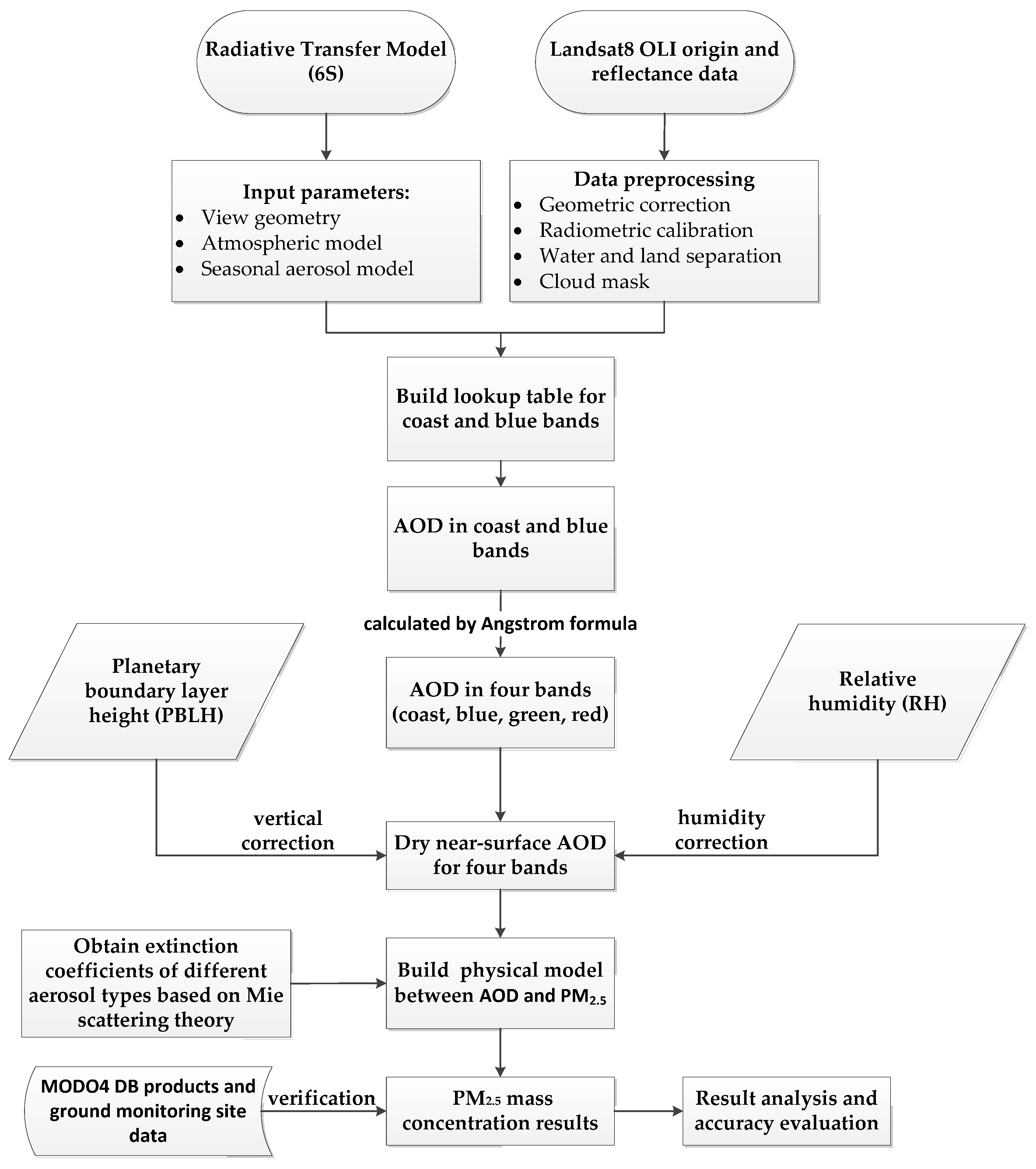
The workflow of our proposed method is shown in Figure 2. First, Landsat8 OLI data preprocessing was performed, and the input parameters of the Second Simulation of the Satellite Signal in the Solar Spectrum (6S) model were set to generate a lookup table for the coast and blue bands. Second, according to the generated lookup table, the surface reflectance and apparent reflectance data were brought into the radiation transmission model to obtain the AOD of the coast and blue bands, and then the Angstrom formula was used to derive the AOD of the green and red bands. Third, vertical correction and humidity correction were performed using PBLH and RH data based on the entire atmospheric AOD to obtain dry near-surface AOD. Fourth, a physical model between the dry near-surface AOD and PM2.5 mass concentrations was established based on Mie scattering theory. Fifth, the PM2.5 mass concentration was solved by using multiband dry near-surface AOD. Finally, result analysis and error estimation were performed on the AOD and PM2.5 retrieval results.

Figure 2.
Technical flow chart of PM2.5 mass concentration estimation.
2.2.1. AOD Retrieval Algorithm
This paper used radiative transfer theory to retrieve AOD from satellite remote sensing imagery. Spectral information received by the satellite was the combined effect of the extinction of all substances in the Earth’s atmosphere and the reflection on the ground. The reflectance at the top of the atmosphere (TOA) received by the satellite sensor can be expressed by the following equation [37]:
In the formula, is the solar zenith angle, is the view zenith angle, is the relative azimuth angle, λ is the corresponding sensor band, represents the TOA, representes the atmospheric path radiation reflectance, is the hemisphere albedo in the atmosphere, and represent the atmospheric upward transmittance and downward transmittance, respectively, and represents the surface reflectance. To solve Equation (1), this study adopted the 6S model to simulate the transmission process of light in the atmosphere. By setting the imaging time, view geometry, specific band, atmospheric model, aerosol type, and surface reflectivity, the model simulates the radiative transmission process in the atmosphere at the time input, and then under different AODs is simulated by three key parameters:, and . Finally, the AOD can be obtained by comparing the real and simulated TOA.
2.2.2. Aerosol Model Determination
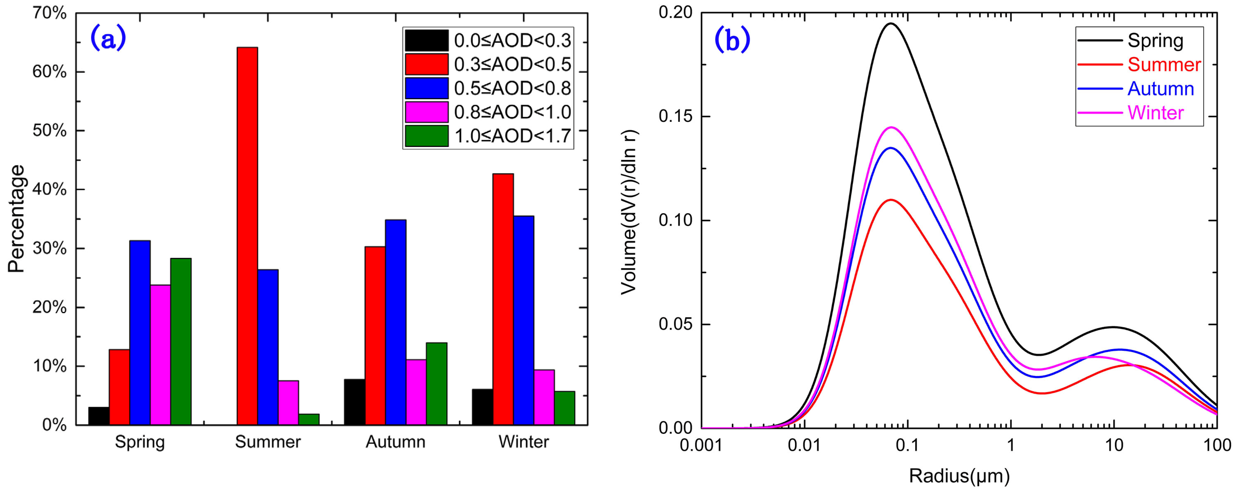
When using the 6S model to generate a lookup table, there were two important input parameters: The surface reflectance (the surface reflectance problem was solved by downloading it from the USGS) and the aerosol model. Related research shows that the aerosol model has a significant impact on the retrieval of AOD [38]. In this study, three years (2017–2019) of Sun photometer data from the CE318 instrument were used to determine the aerosol model. The site was located on the South Campus of Sun Yat-sen University at a longitude of 113°06′12″ E and a latitude of 23°06′12″ N. Through simple data processing and classification, AODs at 550 nm in different seasons (spring: March–May; summer: June–August; autumn: September–November; winter: December–February) were obtained. Figure 3a shows that the proportion of AOD between 0 and 0.3 in each season was relatively low throughout the year, while the proportion of AOD between 0.3 and 0.5 was highest in summer and lowest in spring. The proportion of AOD between 0.5 and 0.8 was relatively high and was approximately 30% in each season. The proportions of AOD in the intervals from 0.8–1.0 and 1–1.7 were highest in spring and lowest in summer, and the proportions of AOD in these intervals in summer were lower than the annual averages. This also reflected that the AOD in Guangzhou was higher in spring, reached a lower level in summer, and rebounded in autumn and winter. Then, aerosol particles were divided into four types (water-soluble, dust, marine, soot) based on the SRA model in this paper. To obtain the volume ratio of different aerosol particles, a Monte Carlo forward modeling method was adopted to determine the aerosol model by using processed AOD data in various bands [39,40], which mainly consisted of two steps. Firstly, we randomly generated the volume ratio of three particles were , , (all values were between 0 and 1), and the volume ratio of the other particle was = 1 − (the value of must be between 0 and 1), and then substituted them into the Equation (19) to calculate the simulated AOD of different bands. Secondly, a comparison was made between the simulated AOD and real AOD retrieved by the satellite. When their differences meet a certain accuracy range, , , , and can be considered as the correct volume ratio of aerosol particles, then the aerosol model will be finally determined.
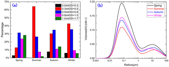
Figure 3.
(a) The statistical distribution of AOD percentages and (b) average volume size distributions of particulates in different seasons.
The distribution of average particle volumes in different seasons is shown in Figure 3b. The structural ratios of aerosol components in different seasons are shown in Table 3. Generally, the volumetric proportions of various components of aerosol particles were stable and did not change with the season, indicating a relatively fixed pollution source, and the particle volume distribution showed a bimodal structure that was mainly composed of water-soluble and soot particles with sizes less than 0.1 μm. According to the definitions of the SRA model, the aerosol model in the PRD is a mixed structure of urban industrial and ocean type. Therefore, when inputting the aerosol model parameters based on the 6S model, according to the transit season of the satellite image, an accurate AOD can be obtained by inputting the proportions of various components of aerosol particles corresponding to Table 3.

Table 3.
The percentages and average concentrations of aerosol particles by volume in different seasons from 2017 to 2019 over the PRD.
2.2.3. Multiband AOD Retrieval
After the aerosol model and surface reflectance were determined, the intervals and ranges of some input parameters (such as view geometry, AOD, atmospheric model, band) were set to generate a lookup table by using the 6S model. The details of these input parameters are listed in Table 4. The generated lookup table of the coast and blue band contains seven columns of values (, , , , , , AOD). For the AOD retrieval of these two bands, the lookup table of the corresponding band was selected, and the corresponding parameters (,,) were derived by obtaining the view geometric information (, , ) of each pixel. Then, it was substituted into equation (1) to obtain the simulated TOA. The real AOD can be interpolated by comparing the real and simulated TOA. In this way, the coast and blue bands of AOD can be obtained accurately in this study, and then the green and red bands of AOD can be obtained by the Angstrom equation [41]:
where is the AOD at different wavelengths, is the wavelength index, and represents the Angstrom turbidity coefficient. If the AOD of two wavelengths was obtained, and can be expressed as:

Table 4.
The input parameters used to generate the lookup table.
Substituting and into Equation (2), the AOD of other wavelengths can be derived.
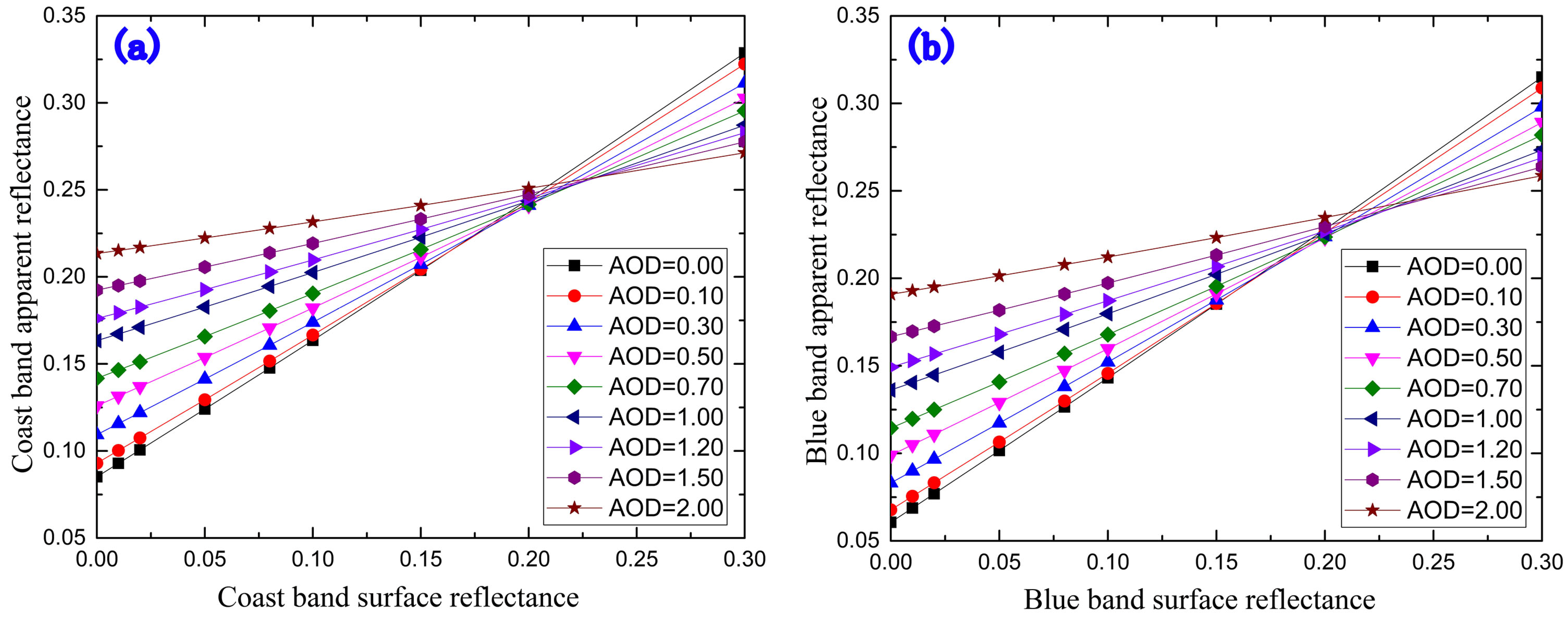
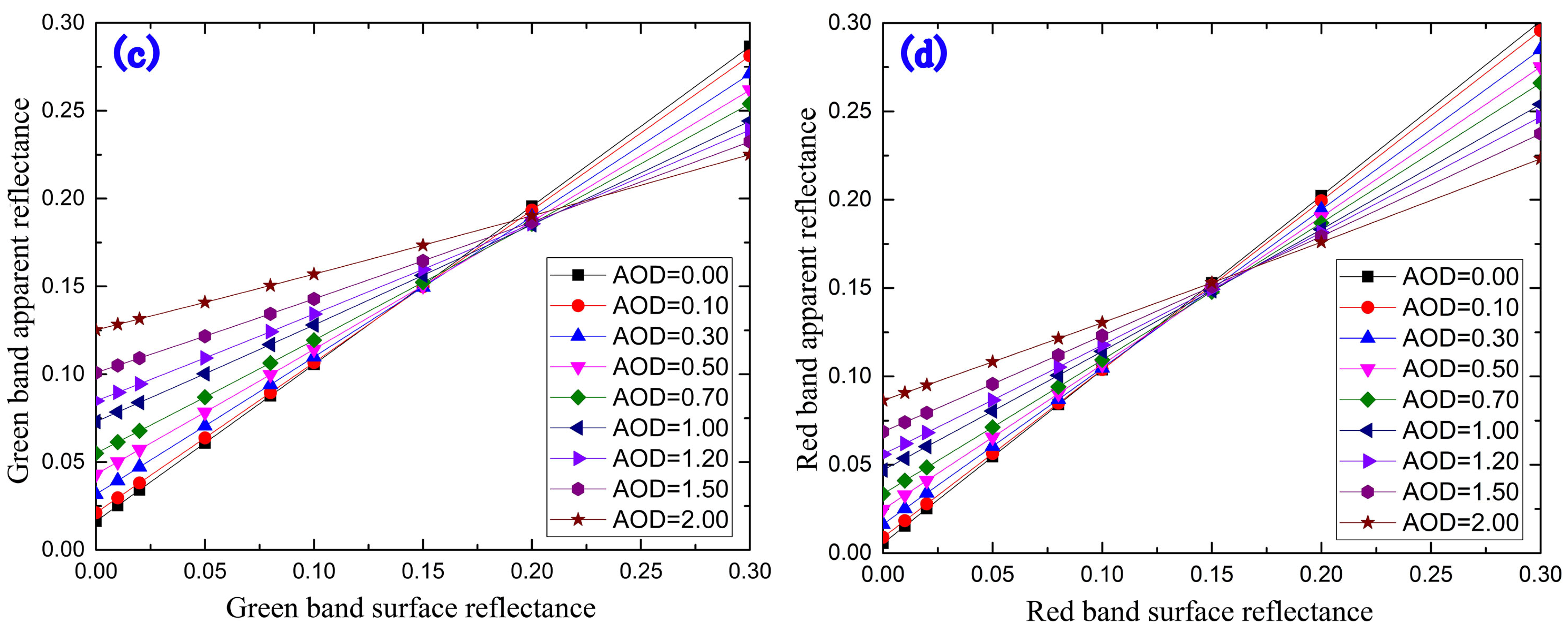
In addition, to demonstrate the feasibility of AOD retrieval for various bands of Landsat8 OLI, the changes in the sensitivity of the TOA to the surface reflectance at different AOD values were analyzed by using the 6S model. In the simulation, the view geometry was set as , °, and = 120°, and the aerosol model and atmospheric model were set as custom and mid-latitude winter model respectively. Figure 4 shows that the TOAs of the four bands were all sensitive to the surface reflectance, and there was a threshold point at a surface reflectance of 0.2. When the surface reflectance was less than 0.2, the TOA increased with increasing AOD. When the surface reflectance was greater than 0.2, the TOA decreased with increasing AOD. When the surface reflectance was fixed, it can be seen from Figure 4 that the TOA was gradually insensitive to changes in AOD as the wavelength increased, especially in the red band, the TOA changed very little with the growth of AOD. Therefore, it was reasonable to choose the coast and blue bands to retrieve AOD in this paper.
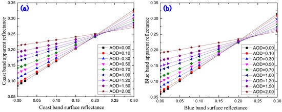
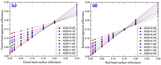
Figure 4.
The sensitivity analysis of TOA in different bands ((a) coast band; (b) blue band; (c) green band; (d) red band) to surface reflectance and AOD.
2.2.4. PM2.5-AOD Model Building
The AOD of four bands over the entire atmospheric column (AODcolumn), representing the extinction of all aerosol particles in the vertical direction, is obtained through the above steps. However, the result measured by the ground monitoring site is the PM2.5 value near the surface under dry conditions. In order to establish the relationship with the PM2.5 mass concentration monitored on the ground, the vertical correction and humidity correction should be performed on AODcolumn to obtain the near-surface dry AOD. The vertical correction, is achieved by assuming that the aerosol vertical distribution follows a negative exponential form, then the near-surface AOD can be derived using the following equation [42,43]:
where represents the near-surface AOD at wavelength λ (in units of μm−1), z is the vertical height (in units of km), and H is the aerosol scale height (in units of km), which can be approximated by the PBLH [44]. Regarding the humidity correction, it is necessary to obtain the extinction properties of dry particles and the aerosol particle hydroscopic growth function (with no unit), which have been studied for a long time [45,46,47]. The aerosol particle hydroscopic growth function can be expressed by the following equation:
where is the relative humidity of the atmosphere at ground level (with no unit) and and represent the dry and wet radii, respectively. The values of a and b can be found in the related literature [48]. Then, the optical hydroscopic growth function can be expressed as:
Then the near-surface dry AOD can be expressed by the following equation [49,50]:
where (in units of μm−1) is the near-surface dry AOD at wavelength λ. and then the of the four bands can be obtained. Assuming that all particles in the atmosphere are spherical particles, according to Mie scattering theory, the near-surface dry AOD () can be expressed as [51,52,53]:
where is the extinction coefficient of a single particle (with no unit), is the particle radius (in units of μm), is the upper limit radius of extinction particles, is the wavelength (in units of μm), represents the particle complex refractive index, which is composed of real and imaginary parts, and is the aerosol particle size distribution (in units of μm−4). Defining , Equation (8) can be rewritten as:
was defined as the aerosol particle size distribution weight function (in units of μm2). For the volume distribution of aerosol particles, based on , , was defined as the aerosol particle volume distribution weight function (in units of μm−1). Then, Equation (9) can be changed to:
where is the aerosol particle volume distribution (in units of μm−1). The complex normal logarithmic volume distribution, which can describe various aerosol modes, was chosen to simulate the particle volume distribution in this study [54]. Aerosol particles are divided into four types based on the SRA model: Water-soluble, dust, marine, and soot. Each aerosol type is composed of aerosol components in different proportions. The specific expression is as follows:
where (i = 1, 2, 3, 4) represents the water-soluble, dust, marine, and soot particle volumes, is the standard deviation of different particle radii, and is the mean volume median radius (in units of μm). The values of parameters are shown in Table 5.

Table 5.
SRA model parameters for different aerosol types [55].
To solve Equation (10), the weight function must be obtained. The key is to know the extinction coefficient , which can be calculated by the following equation based on Mie theory [56]:
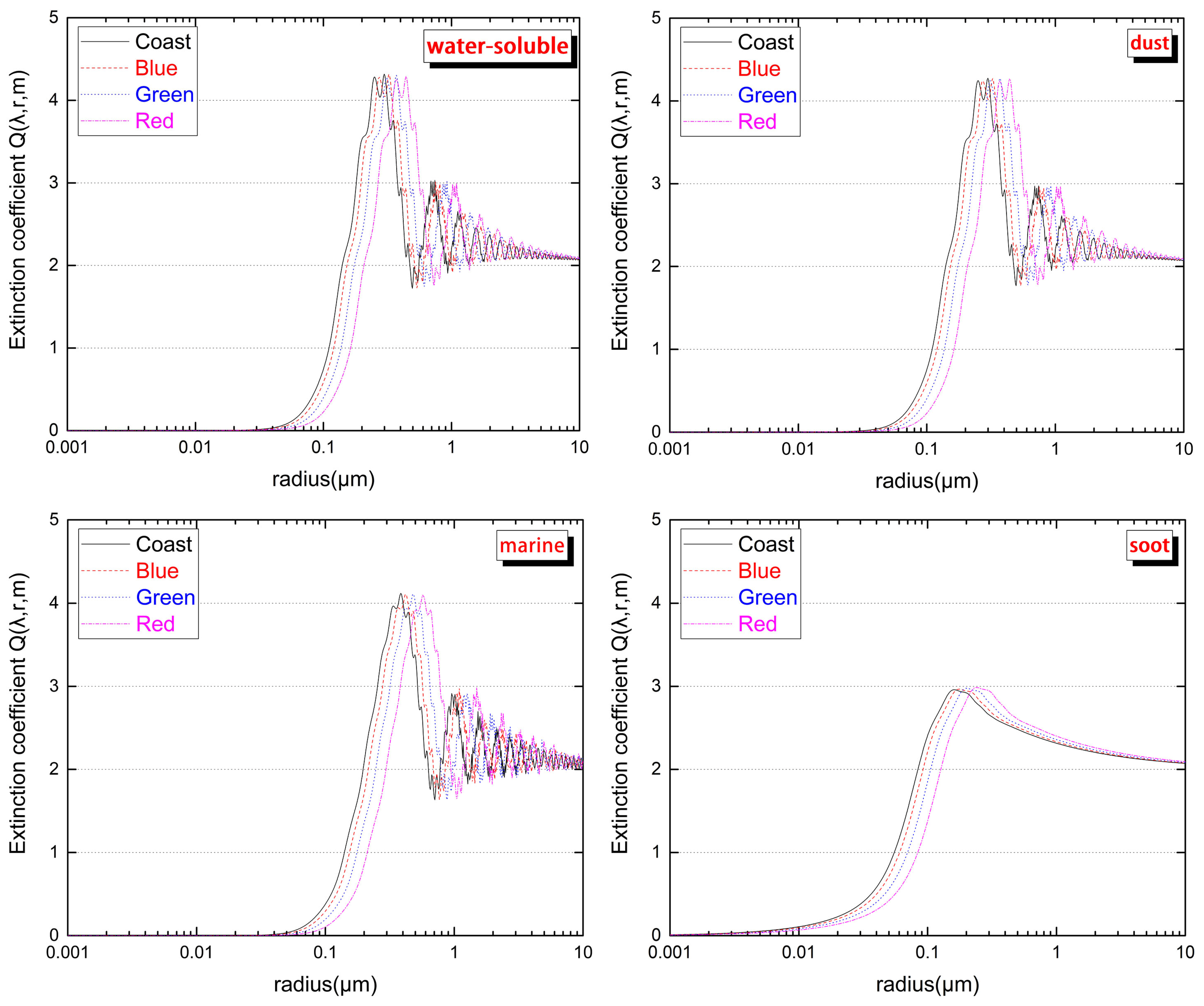
where , representing the scale parameter, and and are Mie scattering parameters that are related to the complex refractive index of the particle. The extinction coefficient of different aerosol particles is derived by obtaining the complex refractive index of these four particles [55]. Figure 5 shows that the extinction coefficient of different aerosol components varies with particle radius at the center wavelength of different bands. The trends of different bands were the same, but the peaks gradually moved to the shortwave direction for different bands. With increasing particle radius, the extinction coefficient oscillated and converged to 2. Then, the volume weight function can be determined based on the previous definition.
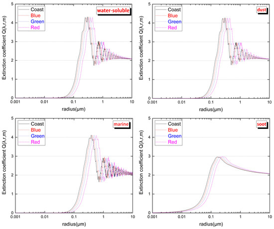
Figure 5.
The extinction coefficient of different aerosol particles at different bands.
If the at different bands are known, the volume distribution can be solved by specific methods. Then, the mass concentration of PM2.5 can be expressed as:
where represents the dry mass density of fine particles near the ground (in units of g/cm3). The value of in the PRD can be found in the relevant literature [57].
2.2.5. Volume Distribution Solution
Combining Equations (10) and (11) yields the following equation:
where is the volume weight function of different aerosol particles (i = 1, 2, 3, 4 represent water-soluble, dust, marine, and soot). Then, the definite integral is discretized, and the complex trapezoidal formula is taken:
where ,. The values of and depend on the extinction radius range of different aerosol particles, and Figure 5 shows the range is from 0.01 μm to 10 μm because when the radius is less than 0.01, the extinction coefficient tends to 0, and when the radius is greater than 10, the extinction coefficient oscillates and converges to 2. In addition, n is the degree of discretization with a value of 1000 in this study, so . Assuming that the total volume of aerosol particles per column is V and that the volumetric proportion of four aerosol particles is and satisfies (i=1, 2, 3, 4 represent water-soluble, dust, marine, and soot), the volume distribution of different particles can be expressed as:
Equation (17) is defined as:
Substituting Equation (17) into Equation (15):
Equation (19) is defined as:
can be calculated by these known parameters, denoted as , which is a 4*1 matrix. Then, Equation (19) can be converted as:
There are four variables in Equation (18) because satisfied . Equation (20) will be solved by the of the four bands obtained earlier and then substituted into Equation (16) to obtain . Finally, the PM2.5 mass concentrations can be obtained through Equation (13).
2.2.6. Model Evaluation
We used two kinds of data to verify the AOD and PM2.5 evaluation results. One was MODO4 DB AOD (550 nm) products, which were used to verify the Landsat8 OLI AOD (550 nm) retrieval results synchronously. Only if the retrieval results of AOD (550 nm) are reliable can the evaluation of PM2.5 be accurate. The second was ground monitoring site PM2.5 data; there were 52 ground monitoring stations in the study area, and the hourly average values were used to verify the estimated PM2.5 results. In addition, the root mean square error (RMSE) was used as an evaluation index for the AOD and PM2.5 results. The overall uncertainty of the model was evaluated using error propagation theory [58,59], and the errors of PM2.5 can be written as:
3. Results
3.1. Retrieved Results from the Proposed Model
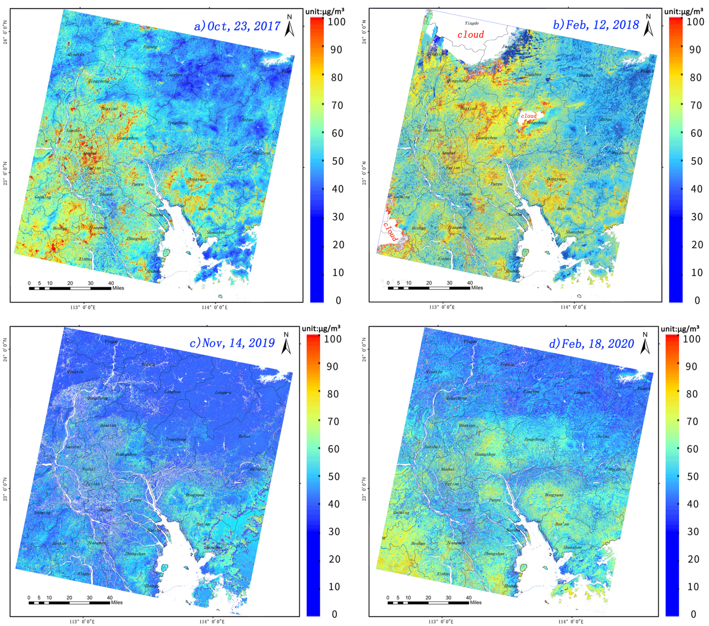
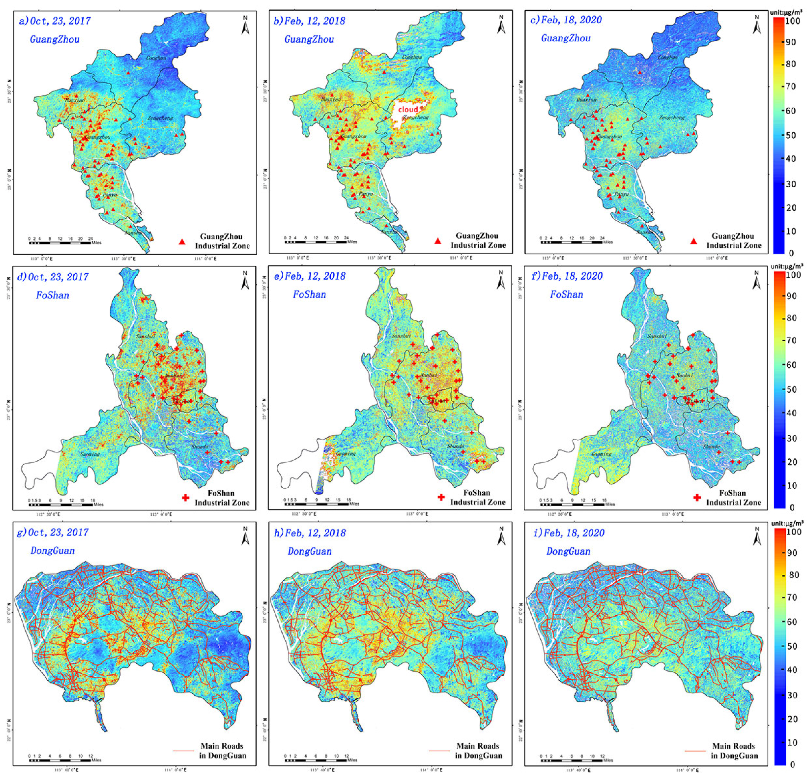
Using the physical model proposed above, the four-year Landsat8 OLI images of the PRD area in spring and winter were selected as the retrieval target because more rainfall leads to poor data in summer and autumn. The cloud coverage of all images was less than 10%, which was convenient for better retrieval results. In addition, water and land separation and cloud mask extraction were carried out before inversion, and no inversion was performed in the areas of water and clouds. Figure 6 shows the temporal and spatial distributions of Landsat8 OLI PM2.5 in the PRD for a certain day in different years. The PM2.5 mass concentrations on 12 February 2018 was higher than on 23 October 2017, and the pollution range was relatively wide on 12 February 2018, improved on 14 November 2019, and expanded again on 18 February 2020. The results on 23 October 2017 and 23 October 2018 showed that the PM2.5 pollution in the PRD region has a wide range, mainly distributed in Foshan, Guangzhou, Shenzhen, and Dongguan, which are highly industrialized cities. Lower pollution areas were mainly distributed in northern Guangdong, and the heavily polluted areas even exceeded 100 μg/m³. The results on 14 November 2019 showed that there was no large-scale pollution, and only a few regions had high PM2.5 values. However, PM2.5 pollution in the PRD has become more serious again since 18 February 2020, such as in Gaoming, Heshan, and Xinhui, which are distributed in southwestern Guangdong and are experiencing certain pollution.
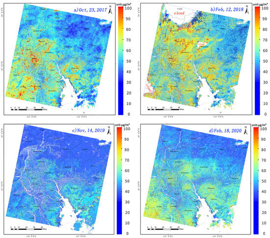
Figure 6.
Spatial and temporal distribution of PM2.5 mass concentrations in the PRD for a certain day in different years.
In addition, the pollution sources of several major industrial cities in the PRD can be identified through the ultrahigh resolution retrieval results of PM2.5 concentrations. Therefore, the areas with high PM2.5 values in three years (except for 14 November 2019) were used to analyze the pollution status of Guangzhou, Foshan, and Dongguan cities.
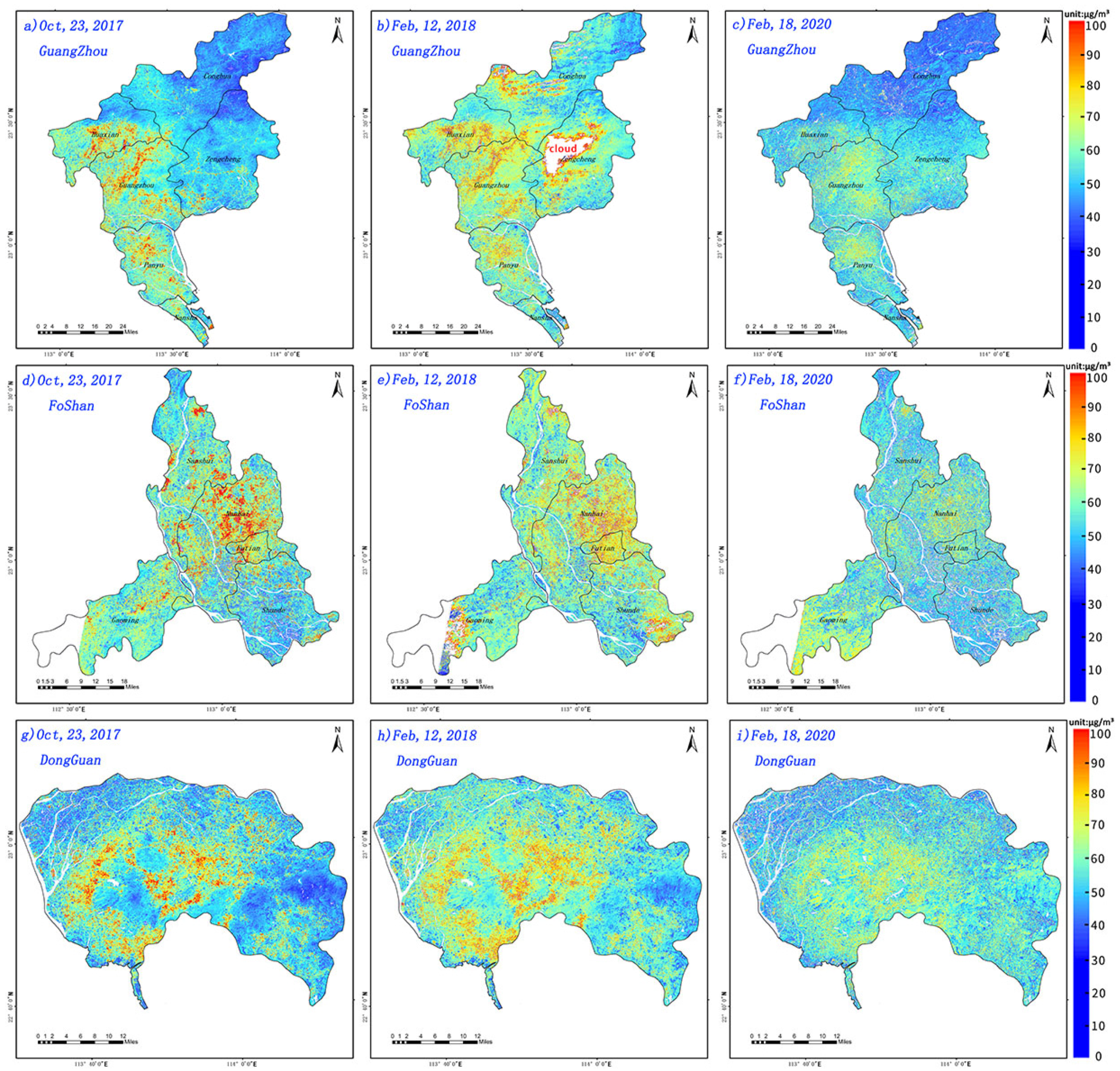
Figure 7 shows that the PM2.5 mass concentrations in downtown Guangzhou and Panyu District were relatively high, and the PM2.5 mass concentrations for different days in the three years reached 80 μg/m³ or more, while the Zengcheng and Conghua Districts in northern Guangzhou were relatively lightly polluted. The areas with high PM2.5 mass concentrations in Foshan city were mainly distributed in Nanhai District and Sanshui District. The PM2.5 mass concentrations in Nanhai District exceeded 100 μg/m³ on 23 October 2017. The overall pollution area in Dongguan was relatively large and unevenly distributed. The main pollution areas were concentrated in western, central, and southeastern Dongguan. Relative to other parts of the study area, areas adjacent to Guangzhou and Shenzhen were seriously polluted. Through the above ultrahigh resolution PM2.5 retrieval results in different cities, the range of urban scale pollution can be clearly known.

Figure 7.
The spatial and temporal distribution of PM2.5 mass concentrations in Guangzhou, Foshan, and Dongguan for a certain day in different years.
3.2. Comparison of Landsat8 OLI AOD with MODO4 DB AOD
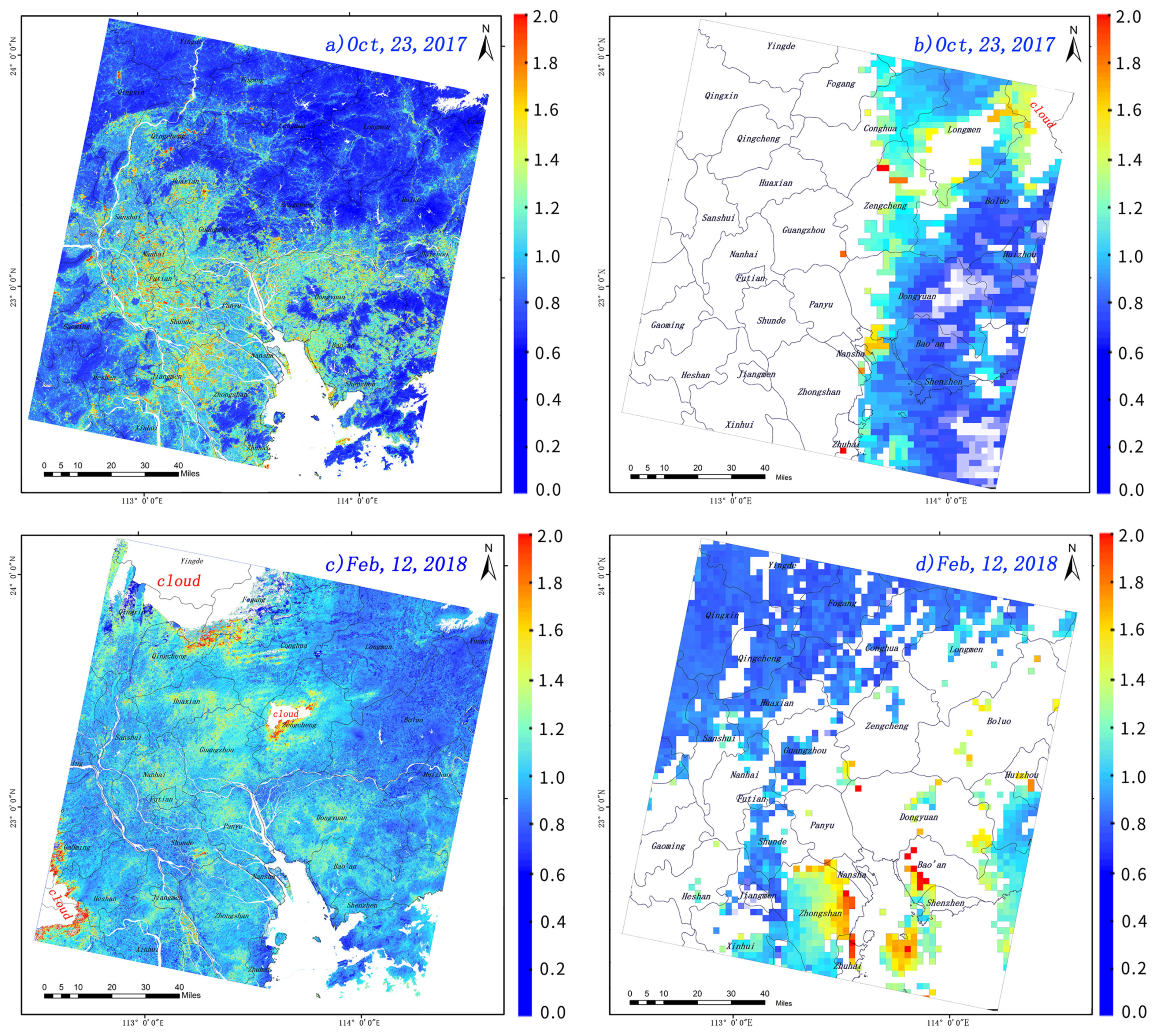
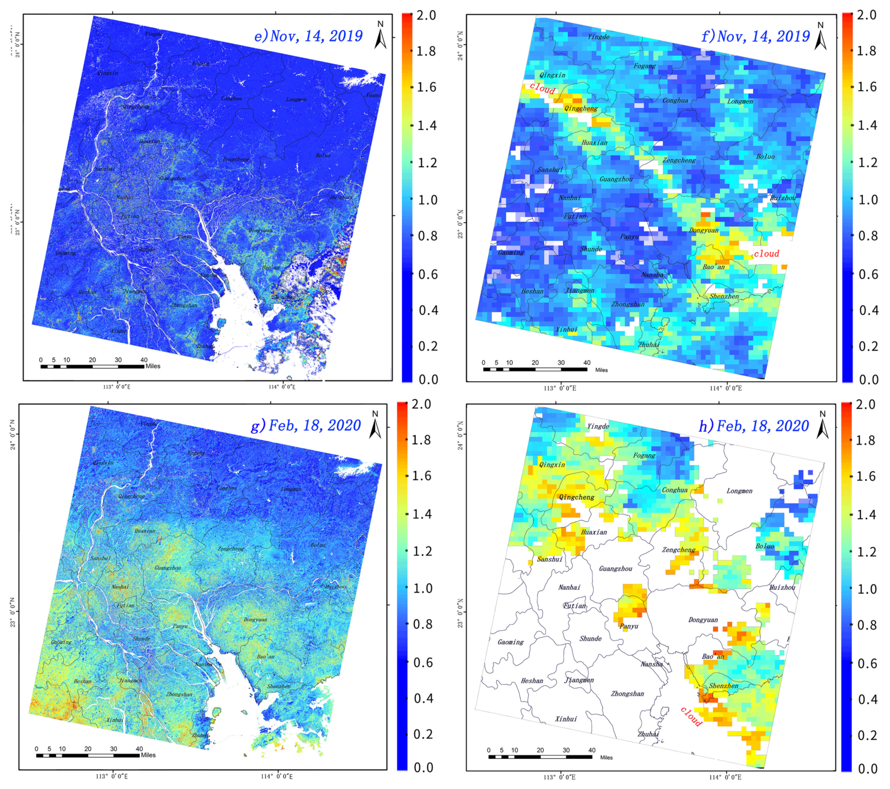
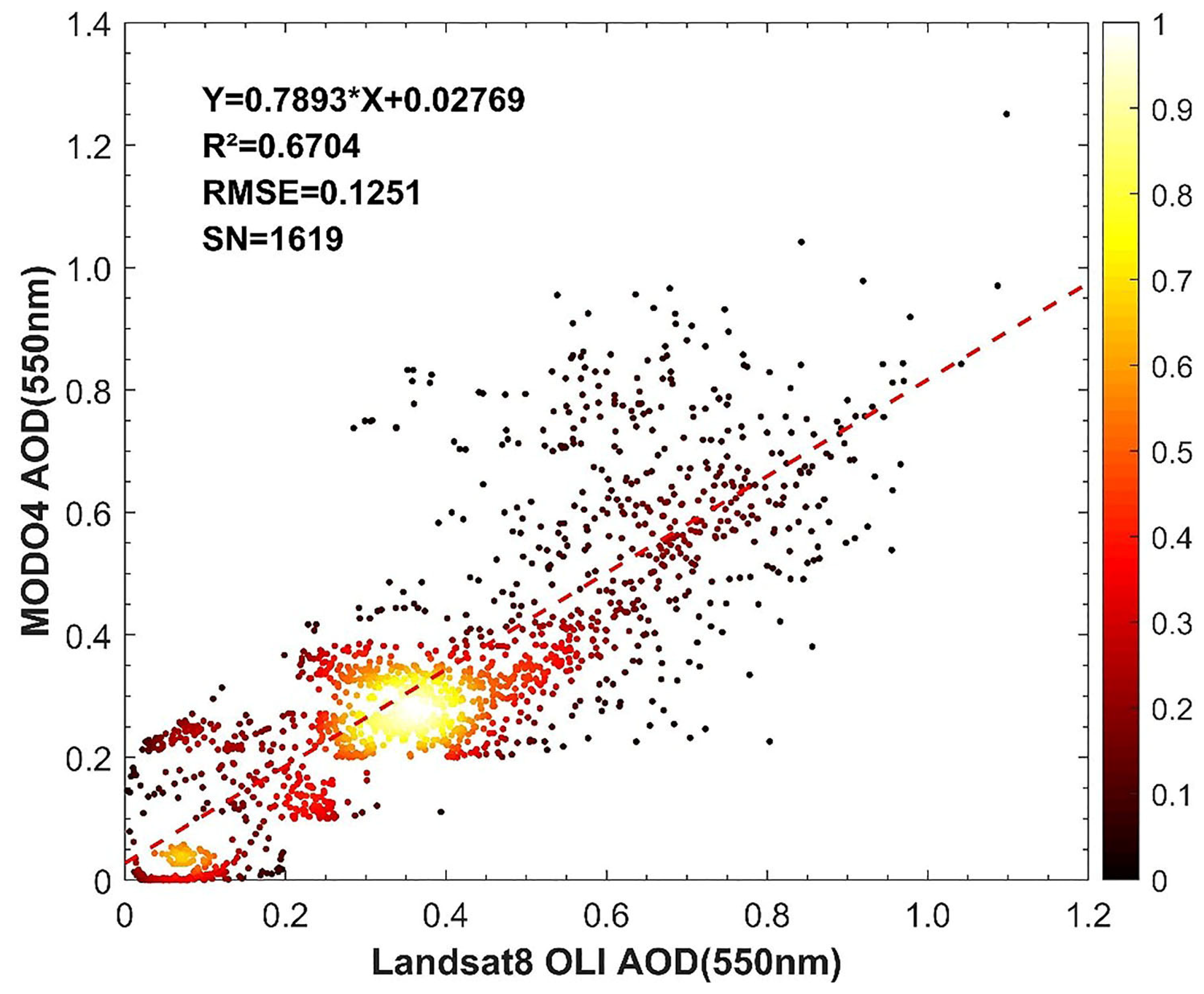
Figure 8 presents the spatial and temporal distributions of Landsat8 OLI AOD (left) and MODO4 DB AOD (right) in the PRD for a certain day in different years. We compared MODO4 DB AOD and Landsat8 OLI AOD and found that Landsat8 OLI AOD tended to be slightly higher than MODO4 DB AOD, which may be caused by different resolutions or a slight difference in transit time. In addition, MODO4 DB AOD products sometimes lack too much area and cannot provide abundant details, due to their coarse resolution (3 km); nevertheless, Landsat8 OLI AOD at a spatial resolution of 30 m can satisfy the needs of urban scale monitoring. To further verify the correlation between the MODO4 DB AOD and Landsat8 OLI AOD, we resampled Landsat8 OLI AOD to the same resolution as MODO4 DB AOD and then conditionally picked verification points in the area that had MODO4 DB AOD data for comparison. In the process of selecting verification points, to avoid areas with high MODO4 DB AOD values caused by clouds and MODO4 DB AOD areas above waters, we eliminated verification points with high AOD values (greater than 1.5), so that they better match with Landsat8 AOD for verification. Figure 9 shows a reasonable relationship with a correlation coefficient (R2) of 0.66 and RMSE of 0.1037 between Landsat8 OLI AOD and MODO4 DB AOD at 550 nm. The slope (0.7893) was less than 1, indicating that Landsat8 OLI AOD was generally higher than MODO4 AOD. The MODO4 DB AOD was slightly larger than the Landsat8 OLI AOD only when the Landsat8 OLI AOD was small.

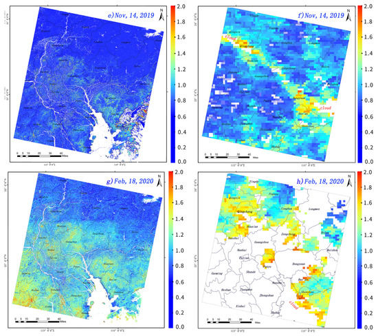
Figure 8.
Spatial and temporal distribution of Landsat8 OLI AOD (Left) and MODO4 DB AOD at 3 km (Right) in the PRD for a certain day in different years.

Figure 9.
Relationship between Landsat8 OLI AOD and MODO4 AOD at 550 nm. RMSE and SN represent the root mean square error and total sample number of matched pixels, respectively.
3.3. Comparison Landsat8 OLI PM2.5 with Ground Measurements
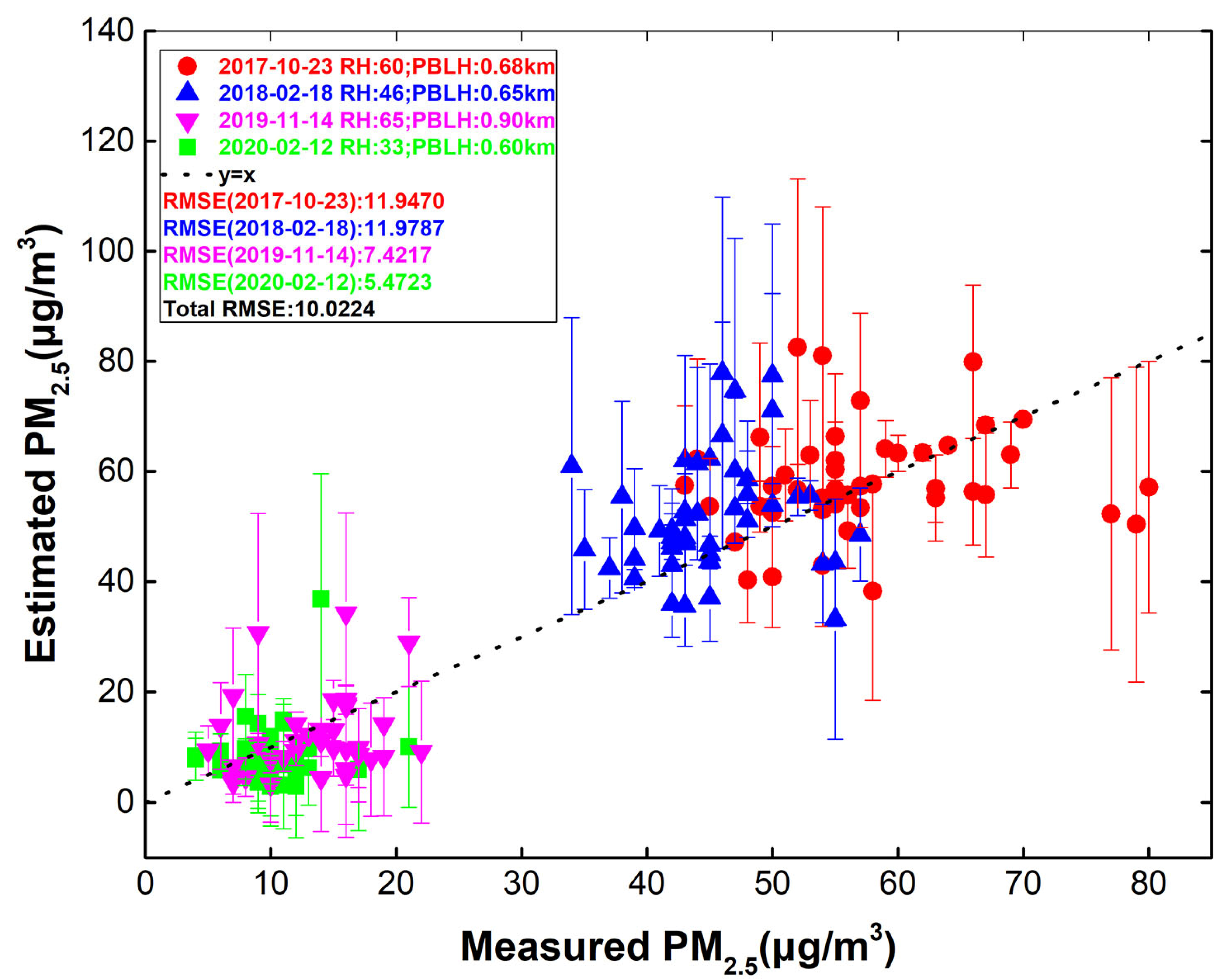
PM2.5 data from ground monitoring sites were used to verify the accuracy of the retrieval results. The time difference between the ground monitoring sites and satellite transit time was less than 30 minutes, and the average PM2.5 value of 3 × 3 pixels around the ground monitoring site was compared with the PM2.5 value of the ground monitoring site. Figure 10 shows the PM2.5 absolute error diagram between the estimated results and measured results. The total RMSE was 10.0224 μg/m³. The RMSEs of a certain day in different years, including 2017, 2018, 2019, and 2020, were 11.9470 μg/m³, 11.9787 μg/m³, 7.4217 μg/m³, and 5.4723 μg/m³, respectively. When the PM2.5 value was approximately 50 μg/m³, the relative error was the smallest. When the PM2.5 value was greater than 60 μg/m³, the error increased. Among the evaluation results of the four years, the results from 14 November 2019 and 18 February 2020 were more accurate; in contrast, on 23 October 2017 and 12 February 2018, severe air pollution led to poor accuracy. The overall error of AOD and PM2.5 was small, which reflected the feasibility of the algorithm.
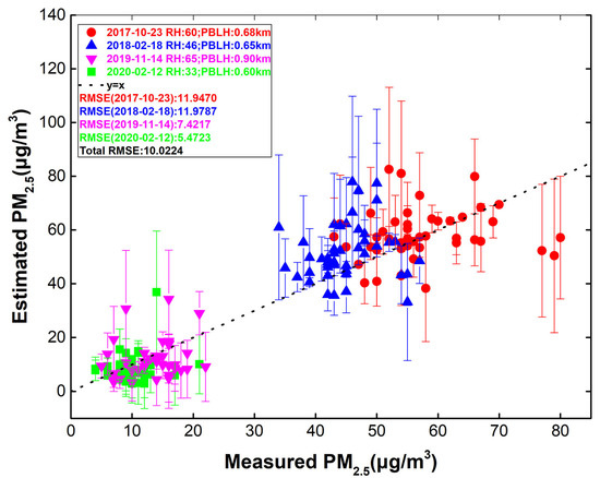
Figure 10.
PM2.5 absolute error diagram between ground monitoring station measurements and estimated results for a certain day in different years.
3.4. Error Estimation
This study was based on multiband AOD to establish a physical model of PM2.5 mass concentration retrieval. Therefore, the main error comes from the multiband AOD and the parameters in the physical model. The model parameterization error mainly comes from . The average uncertainty in the hygroscopic growth item was estimated to be 24%, according to Table 6. Water and land separation was performed based on the Landsat8 OLI datasets, so the uncertainty of urban or mixed aerosols was reduced to 12%, as shown in Table 6. The uncertainty of AOD was determined by the comparison between Landsat8 OLI AOD and MODO4 DB AOD at 550 nm. Section 3.2 shows that the relative error between the two was 0.1251. In addition, the fine particle density can also vary in different regions. This study adopted 1.5 g/cm³ as the fine particle density in the PRD region, which produced an error of approximately 28% compared with the national average fine particle mass density of 2.09 g/cm³ [59]. In summation, the total uncertainty of PM2.5 was approximately 33% following equation (21). The uncertainty of parameters, such as PBLH and RH, depends greatly on the sensors and retrieval algorithm and needs improvement in future work.

Table 6.
Hygroscopic growth functions on particle radius (r) and particle extinction (o). The error column shows the difference between two hygroscopic growth functions and [29].
4. Discussion
This paper presented a new physical model based on multiband AOD for PM2.5 estimation. The results showed ultrahigh spatial resolution and abundant spatial details, which can be applied to urban scale atmospheric monitoring and can be combined with other geographic data to analyze pollution characteristics in different cities. Figure 11a–i shows the pollution characteristics of the three major industrial cities (Guangzhou, Foshan, and Dongguan) in the PRD of a certain day in different years. The pollution in Guangzhou (Figure 11a–c) and Foshan (Figure 11d–f) was mainly industrial pollution, and the denser industrial zones had higher PM2.5 values. The pollution characteristics of Dongguan were linearly distributed along the roads, indicating that traffic pollution was the main cause, which was very similar to the pollution situation in northern Poland [60]. With the previous coarse resolution PM2.5 retrieval results, which pay more attention to PM2.5 estimation at a large scale, it is difficult to obtain pollution characteristics at the urban scale. The ultrahigh resolution retrieval results from this approach can be provided to the urban environmental department to support better regulatory measures.

Figure 11.
Analysis of pollution characteristics of the three major industrial cities (Guangzhou: (a–c); FoShan: (d–f); DongGuan: (g–i)) in PRD for a certain day in different years.
However, there were still some limitations and deficiencies in this study. The first was that long-term ground monitoring data were needed to determine the aerosol mode in the study area; otherwise, it was difficult to obtain accurate AOD, which had a great impact on the subsequent PM2.5 retrieval. The second was that the simple aerosol vertical distribution function had difficulty representing the vertical distribution of aerosols in the entire PRD area, and the uniform use of the negative exponential distribution function inevitably caused errors in the retrieval results. Third, this study used Mie scattering theory to simulate the extinction characteristics of different aerosol particles, which varied from the extinction characteristics of real aerosol particles in the atmosphere. Measurement experiments of extinction characteristics should be performed on different types of aerosols in the study area to obtain their true extinction characteristics, which will make the physical model of PM2.5-AOD more suitable for the real conditions in the study area.
5. Conclusions
In this study, we used Landsat8 OLI images to retrieve the AOD of the coast and blue bands based on the 6S model, and then the Angstrom formula was used to obtain the AOD of the green and red bands. Then, the dry near-surface AOD of visible bands was obtained through vertical correction and humidity correction, and the aerosol particles in the PRD were divided into four different types according to the SRA model. The extinction characteristics of different types of aerosol particles were simulated by the Mie scattering theory. Finally, a physical model was established between PM2.5 and dry near-surface AOD to obtain the spatial and temporal distribution characteristics of PM2.5 in the PRD. The resolution of the retrieved results was the same as that of the original images, and the distribution of PM2.5 at the urban scale was analyzed by using ultrahigh resolution remote sensing results. The retrieval results showed the distribution of PM2.5 mass concentrations in the PRD for a certain day in different years, and the cities with higher degrees of industrialization (such as Guangzhou, Foshan, and Dongguan) were analyzed in detail. The urban areas of Guangzhou and Panyu District had high pollution except on 14 November 2019, and the PM2.5 mass concentrations exceeded 80 μg/m³. The pollution in Foshan was mainly in Nanhai District, while the PM2.5 mass concentrations in Dongguan were mainly distributed in the western, central, and southeastern regions. In addition, ultrahigh resolution retrieval results were also used to analyze the pollution characteristics of different cities on the day; the industrial pollution was dominant in Guangzhou and Foshan, while traffic pollution was the main factor in Dongguan which was consistent with other studies on pollution characteristics of industrial cities [61,62]. Finally, the retrieval results were verified by using MODO4 DB AOD products and ground monitoring station data. The AOD at 550 nm retrieved in this study had high consistency with MODO4 DB AOD products. The RMSE of the PM2.5 mass concentration retrieval results and ground monitoring station results was only 10.0224 μg/m³, which indicated that the retrieval results were reliable.
It should be mentioned that the resolution of parameters, such as PBLH and RH, used in this study was 0.125° × 0.125°, which was different from the resolution of Landsat8 OLI data. Corresponding errors are introduced when making the humidity correction and vertical correction. In addition, the 30 m AOD retrieval result was resampled to 3 km for verification with the 3 km MODO4 DB AOD products, which introduces certain verification errors. Despite some limitations, our proposed physical model can still provide some information support to urban environmental departments. In the future, we will carry out a quantitative comparison based on the vertical profile of the dissipation coefficient by Landsat8 and CALIPSO [63] and the generation of PBLH images covering the original images [64,65] or use Lidar to perform multipoint measurements of the study area to obtain an accurate vertical distribution of aerosols, which will greatly improve the vertical correction [66]. In addition, we will also conduct different types of aerosol extinction coefficient measurements in the study area to improve the model.
Author Contributions
Conceptualization, Y.T. and R.D.; Software, Y.T. and R.Z.; Data Curation, Y.T. and Z.H.; Writing—Original Draft Preparation, Y.T. and L.X.; Writing—Review and Editing, J.L. and Y.L. (Yongming Liu); Supervision, J.L and R.D.; Project Administration, R.D.; Funding Acquisition, Y.L. (Yeheng Liang). All authors have read and agreed to the published version of the manuscript.
Funding
National Natural Science Foundation of China (No. 41071230 and 41901352); Science and Technology Planning Project of Guangdong Province, China (No. 2017B020216001); Guangdong Basic and Applied Basic Research Foundation (No. 2020A1515010780); Innovation Projects in Water Resource of Guangdong Province, China (No. 2016-08).
Acknowledgments
We appreciate the support of the European Centre for Medium-Range Weather Forecasts (ECMWF) in providing reanalysis meteorological data. In addition, we sincerely appreciate all the anonymous reviewers for their excellent comments and efforts.
Conflicts of Interest
The authors declare no conflict of interest.
References
- Dockery, D.W.; Pope, C.A. Acute respiratory effects of particulate air pollution. Annu. Rev. Public Health 1994, 15, 107. [Google Scholar] [CrossRef]
- Beelen, R.; Raaschou-Nielsen, O.; Stafoggia, M.; Andersen, Z.J.; Weinmayr, G.; Hoffmann, B.; Wolf, K.; Samoli, E.; Fischer, P.; Nieuwenhuijsen, M.; et al. Effects of long-term exposure to air pollution on natural-cause mortality: An analysis of 22 Europeanm cohorts within the multicentre ESCAPE project. Lancet 2014, 383, 785–795. [Google Scholar] [CrossRef]
- Dockery, D.W.; Xu, X.; Spengler, J.D.; Ware, J.H.; Fay, M.E.; Ferris, B., Jr.; Speizer, F.E. An association between air pollution and mortality in six U.S. cities. N. Engl. J. Med. 2013, 329, 1753–1759. [Google Scholar] [CrossRef] [PubMed]
- Pope, C.A., III; Burnett, R.T.; Thun, M.J.; Calle, E.E.; Krewski, D.; Ito, K.; Thurston, G.D. Lung Cancer, Cardiopulmonary Mortality, and Long-term Exposure to Fine Particulate Air Pollution. JAMA 2002, 287, 1132–1141. [Google Scholar] [CrossRef]
- Li, C.; Hsu, N.C.; Tsay, S.C. A study on the potential applications of satellite data in air quality monitoring and forecasting. Atmos. Environ. 2011, 45, 3663–3675. [Google Scholar] [CrossRef]
- Van, D.A.; Martin, R.V.; Spurr, R.J.; Burnett, R.T. High-resolution satellite-derived PM2.5 from optimal estimation and geographically weighted regression over North America. Environ. Sci. Technol. 2015, 49, 10482–10491. [Google Scholar] [CrossRef]
- Che, H.; Xia, X.; Zhu, J.; Li, Z.; Dubovik, O.; Holben, B.; Goloub, P.; Chen, H.; Estelles, V.; Cuevas-Agulló, E. Column aerosol optical properties and aerosol radiative forcing during a serious haze-fog month over North China Plain in 2013 based on ground-based sunphotometer measurements. Atmos. Chem. Phys. 2014, 14, 2125–2138. [Google Scholar] [CrossRef]
- Gupta, P.; Christopher, S.A. Seven year particulate matter air quality assessment from surface and satellite measurements. Atmos. Chem. Phys. 2008, 8. [Google Scholar] [CrossRef]
- Lin, T.H. To construct an effective coefficient of aerosol size distribution for atmospheric turbidity retrieval. Terr. Atmos. Ocean. 2005, 16, 691–706. [Google Scholar] [CrossRef]
- Janet, N.; Muhammad, B. Validation of MODIS 3 km Resolution Aerosol Optical Depth Retrievals Over Asia. Remote Sens. 2016, 8, 328. [Google Scholar] [CrossRef]
- Sun, K.; Chen, X.; Zhu, Z.; Zhang, T. High Resolution Aerosol Optical Depth Retrieval Using Gaofen-1 WFV Camera Data. Remote Sens. 2017, 9, 89. [Google Scholar] [CrossRef]
- Omari, K.; Abuelgasim, A.; Alhebsi, K. Aerosol optical depth retrieval over the city of Abu Dhabi, United Arab Emirates (UAE) using Landsat-8 OLI images. Atmos. Pollut. Res. 2019, 10, 1075–1083. [Google Scholar] [CrossRef]
- Paciorek, C.J.; Liu, Y. Limitations of Remotely Sensed Aerosol as a Spatial Proxy for Fine Particulate Matter. Environ. Health Perspect. 2009, 117, 904–909. [Google Scholar] [CrossRef]
- Liu, Y.; Sarnat, J.A.; Kilaru, V.; Jacob, D.J.; Koutrakis, P. Estimating ground-level PM2.5 in the eastern United States using satellite remote sensing. Environ. Sci. Technol. 2005, 39, 3269–3278. [Google Scholar] [CrossRef] [PubMed]
- Gupta, P.; Christopher, S.A.; Wang, J.; Gehrig, R.; Lee, Y.; Kumar, N. Satellite remote sensing of particulate matter and air quality assessment over global cities. Atmos. Environ. 2006, 40, 5880–5892. [Google Scholar] [CrossRef]
- Gupta, P.; Christopher, S.A. Particulate matter air quality assessment using integrated surface, satellite, and meteorological products: Multiple regression approach. J. Geophys. Res. Atmos. 2009, 114. [Google Scholar] [CrossRef]
- Engel-Cox, J.A.; Holloman, C.H.; Coutant, B.W.; Hoff, R.M. Qualitative and quantitative evaluation of MODIS satellite sensor data for regional and urban scale air quality. Atmos. Environ. 2004, 38, 2495–2509. [Google Scholar] [CrossRef]
- Kloog, I.; Koutrakis, P.; Coull, B.A.; Lee, H.J.; Schwartz, J. Assessing temporally and spatially resolved PM2.5 exposures for epidemiological studies using satellite aerosol optical depth measurements. Atmos. Environ. 2011, 45, 6267–6275. [Google Scholar] [CrossRef]
- Paciorek, C.J.; Liu, Y.; Moreno-Macias, H.; Kondragunta, S. Spatiotemporal associations between GOES aerosol optical depth retrievals and ground-level PM2.5. Environ. Sci. Technol. 2008, 42, 5800–5806. [Google Scholar] [CrossRef] [PubMed]
- Schaap, M.; Apituley, A.; Timmermans, R.M.A.; Koelemeijer, R.B.A.; de Leeuw, G. Exploring the relation between aerosol optical depth and PM2.5 at Cabauw, the Netherlands. Atmos. Chem. Phys. 2008, 9, 909–925. [Google Scholar] [CrossRef]
- Liu, Y.; Paciorek, C.J.; Koutrakis, P. Estimating regional spatial and temporalvariability of PM2.5 mass concentration using satellite data, meteorology, and land useinformation. Environ. Health Perspect. 2019, 117, 886–892. [Google Scholar] [CrossRef]
- Emili, E.; Popp, C.; Petitta, M.; Riffler, M.; Wunderle, S.; Zebisch, M. PM10 remote sensing from geostationary SEVIRI and polar-orbiting MODIS sensors over the complex terrain of the European Alpine region. Remote Sens. Environ. 2010, 114, 2485–2499. [Google Scholar] [CrossRef]
- Kloog, I.; Nordio, F.; Coull, B.A.; Schwartz, J. Incorporating local land use regression and satellite aerosol optical depth in a hybrid model of spatiotemporal PM2.5 exposures in the mid-Atlantic states. Environ. Sci. Technol. 2012, 46, 11913–11921. [Google Scholar] [CrossRef]
- Xu, J.; Schüssler, O.; Rodriguez, D.G.L.; Romahn, F.; Doicu, A. A Novel Ozone Profile Shape Retrieval Using Full-Physics Inverse Learning Machine (FP-ILM). IEEE J. Sel. Top. Appl. Earth Obs. Remote Sens. 2017, 10, 5442–5457. [Google Scholar] [CrossRef]
- Hong, D.; Yokoya, N.; Xu, J.; Zhu, X. Joint progressive learning from high-dimensional data for multi-label classification. In Proceedings of the European Conference on Computer Vision (ECCV), Munich, Germany, 8–14 September 2018; pp. 469–484. [Google Scholar] [CrossRef]
- Van Donkelaar, A.; Martin, R.V.; Brauer, M.; Kahn, R.; Levy, R.; Verduzco, C.; Villeneuve, P.J. Global estimates of ambient fine particulate matter concentrations from satellite-based aerosol optical depth: Development and application. Environ. Health Perspect. 2010, 118, 847–855. [Google Scholar] [CrossRef] [PubMed]
- Wang, J.; Xu, X.; Spurr, R.; Wang, Y.; Drury, E. Improved algorithm for MODIS satellite retrievals of aerosol optical thickness over land in dusty atmosphere: Implications for air quality monitoring in China. Remote Sens. Environ. 2010, 114, 2575–2583. [Google Scholar] [CrossRef]
- Xu, X.; Wang, J.; Henze, D.K.; Qu, W.; Kopacz, M. Constraints on aerosol sources using GEOS-Chem adjoint and MODIS radiances, and evaluation with multisensor (OMI, MISR) data. J. Geophys. Res. Atmos. 2013, 118, 6396–6413. [Google Scholar] [CrossRef]
- Zhang, Y.; Li, Z. Remote sensing of atmospheric fine particulate matter (PM2.5) mass concentration near the ground from satellite observation. Remote Sens. Environ. 2015, 160, 252–262. [Google Scholar] [CrossRef]
- Lee, H.; Liu, Y.; Coull, B.; Schwartz, J.; Koutrakis, P. A novel calibration approach of MODIS AOD data to predict PM2.5 concentrations. Atmos. Chem. Phys. 2011, 11, 9769–9795. [Google Scholar] [CrossRef]
- Chang, H.H.; Hu, X.; Liu, Y. Calibrating MODIS aerosol optical depth for predicting daily PM2.5 concentrations via statistical downscaling. J. Expo. Sci. Environ. Epidemiol. 2014, 24, 398–404. [Google Scholar] [CrossRef] [PubMed]
- Oo, M.; Ross, A.; Holz, R.; Holloway, T.; Ackerman, S. Investigating cloud contamination in MODIS and VIIRS AOD retrievals and the impacts on air quality applications. AGU Fall Meet. Abstr. 2013, A43D-0296. [Google Scholar]
- Wu, J.; Yao, F.; Li, W.; Si, M. VIIRS-based remote sensing estimation of ground-level PM2.5 concentrations in Beijing–Tianjin–Hebei: A spatiotemporal statistical model. Remote Sens. Environ. 2016, 184, 316–328. [Google Scholar] [CrossRef]
- Liu, Y.; Franklin, M.; Kahn, R.; Koutrakis, P. Using aerosol optical thickness to predict ground-level PM2.5 concentrations in the St. Louis area: A comparison between MISR and MODIS. Remote Sens. Environ. 2007, 107, 33–44. [Google Scholar] [CrossRef]
- Lu, X.; Chen, Y.; Huang, Y.; Lin, C.; Li, Z.; Fung, J.C.; Lau, A.K. Differences in concentration and source apportionment of PM2.5 between 2006 and 2015 over the PRD region in southern China. Sci. Total Environ. 2019, 673, 708–718. [Google Scholar] [CrossRef] [PubMed]
- Wu, Z.; Zhang, Y.; Zhang, L.; Huang, M.; Zhong, L.; Chen, D.; Wang, X. Trends of outdoor air pollution and the impact on premature mortality in the Pearl River Delta region of southern China during 2006–2015. Sci. Total Environ. 2019, 690, 248–260. [Google Scholar] [CrossRef] [PubMed]
- Vermote, E.F.; Tanré, D.; Deuze, J.L.; Herman, M.; Morcette, J. Second simulation of the satellite signal in the solar spectrum, 6S: An overview. IEEE Trans. Geosci. Remote Sens. 1997, 35, 675–686. [Google Scholar] [CrossRef]
- Li, Z.; Niu, F.; Lee, K.; Xin, J.; Hao, W.; Nordgren, B.; Wang, Y.; Wang, P. Validation and understanding of Moderate Resolution Imaging Spectroradiometer aerosol products (C5) using ground-based measurements from the handheld Sun photometer network in China. J. Geophys. Res. Atmos. 2007, 112. [Google Scholar] [CrossRef]
- Wurl, D.; Grainger, R.; McDonald, A.; Deshler, T. Optimal estimation retrieval of aerosol microphysical properties from SAGE II satellite observations in the lower stratosphere. Atmos. Chem. Phys. 2010, 10, 4295–4317. [Google Scholar] [CrossRef]
- Yang, Y.-J.; Fu, Y.-F.; Wu, B.-W.; Shi, C.; Deng, X.-L.; Zhang, H.; Zhang, Y. Impacts of Agricultural Fire on Aerosol Distribution over East China During Summer Harvest Time. J. Atmos. Environ. Opt. 2013, 8, 5–16. [Google Scholar] [CrossRef]
- Angstrom, A. Techniques of Determinig the Turbidity of the Atmosphere. Tellus B 1961, 13. [Google Scholar] [CrossRef]
- Busen, R.; Hänel, G. Radiation budget of the boundary layer, Part1: Measurement of absorption of solar radiation by atmospheric particles and water vapour. Beitraege Zur Phys. Der Atmos. 1987, 60, 229–240. [Google Scholar]
- Lin, C.; Li, Y.; Yuan, Z.; Lau, A.K.; Li, C.; Fung, J.C. Using satellite remote sensing data to estimate the high-resolution distribution of ground-level PM2.5. Remote Sens. Environ. 2015, 156, 117–128. [Google Scholar] [CrossRef]
- Koelemeijer, R.B.A.; Homan, C.D.; Matthijsen, J. Comparison of spatial and temporal variations of aerosol optical thickness and particulate matter over Europe. Atmos. Environ. 2006, 40, 5304–5315. [Google Scholar] [CrossRef]
- Kasten, F. Visibility forecast in the phase of pre-condensation. Tellus 1969, 21, 631–635. [Google Scholar] [CrossRef]
- Tang, I.N. Chemical and size effects of hygroscopic aerosols on light scattering coefficients. J. Geophys. Res. Atmos. 1996, 101, 19245–19250. [Google Scholar] [CrossRef]
- Tang, I.N.; Munkelwitz, H.R. Water activities, densities, and refractive indices of aqueous sulfates and sodium nitrate droplets of atmospheric importance. J. Geophys. Res. Atmos. 1994, 99, 18801. [Google Scholar] [CrossRef]
- Liu, X.; Cheng, Y.; Zhang, Y.; Jung, J.; Sugimoto, N.; Chang, S.-Y.; Kim, Y.J.; Fan, S.; Zeng, L. Influences of relative humidity and particle chemical composition on aerosol scattering properties during the 2006 PRD campaign. Atmos. Environ. 2008, 42, 1525–1536. [Google Scholar] [CrossRef]
- Holben, B.N.; Eck, T.F.; Slutsker, I.a.; Tanre, D.; Buis, J.; Setzer, A.; Vermote, E.; Reagan, J.A.; Kaufman, Y.; Nakajima, T.; et al. AERONET—A Federated Instrument Network and Data Archive for Aerosol Characterization. Remote Sens. Environ. 1998, 66, 1–16. [Google Scholar] [CrossRef]
- Lee, A.K.Y.; Ling, T.Y.; Chan, C.K. Understanding hygroscopic growth and phase transformation of aerosols using single particle Raman spectroscopy in an electrodynamic balance. Faraday Discuss. 2008, 137, 245–263. [Google Scholar] [CrossRef] [PubMed]
- Yamamoto, G.; Tanaka, M. Determination of aerosol size distribution from spectral attenuation measurements. Appl. Opt. 1969, 8, 447–453. [Google Scholar] [CrossRef]
- Nussenzveig, H.M.; Wiscombe, W.J. Efficiency Factors in Mie Scattering. Phys. Rev. Lett. 1980, 45, 1490–1494. [Google Scholar] [CrossRef]
- Bassan, P.; Kohler, A.; Martens, H.; Lee, J.; Byrne, H.J.; Dumas, P.; Gazi, E.; Brown, M.; Clarke, N.; Gardner, P. Resonant Mie Scattering (RMieS) correction of infrared spectra from highly scattering biological samples. Analyst 2010, 135, 268–277. [Google Scholar] [CrossRef] [PubMed]
- Shaw, G.E. On the Aerosol Particle Size Distribution Spectrum in Alaskan Air Mass Systems: Arctic Haze and Non-Haze Episodes. J. Atmos. Sci. 1983, 40, 1313–1320. [Google Scholar] [CrossRef]
- Liou, K.N. An Introduction to Atmospheric Radiation; Academic Press: Cambridge, MA, USA, 2002. [Google Scholar] [CrossRef]
- Hulst, H.C.; van de Hulst, H.C. Light scattering by small particles. Phys. Today 1957, 10. [Google Scholar] [CrossRef]
- Gao, J.; Zhou, Y.; Wang, J.; Wang, T.; Wang, W.X. Inter-comparison of WPSTM-TEOMTM-MOUDITM and investigation on particle density. Environ. Sci. 2007, 28, 1929–1934. [Google Scholar] [CrossRef]
- Rummelhart, D.E.; Hinton, G.E.; Williams, R.J. Learning internal representations by error propagation. Read. Cogn. Sci. 1988, 323, 399–421. [Google Scholar]
- Wang, Y.; Chirikjian, G.S. Second-Order Theory of Error Propagation on Motion Groups. Int. J. Robot. Res. 2006. [Google Scholar] [CrossRef]
- Kwiecień, J.; Szopińska, K. Mapping Carbon Monoxide Pollution of Residential Areas in a Polish City. Remote Sens. 2020, 12, 2885. [Google Scholar] [CrossRef]
- Forehead, H.; Huynh, N. Review of modelling air pollution from traffic at street-level—The state of the science. Environ. Pollut. 2018, 241, 775–786. [Google Scholar] [CrossRef] [PubMed]
- Tsanakas, N. Emission Estimation Based on Traffic Models and Measurements; LiU Tryck: Linköping, Sweden, 2019; pp. 80–85. [Google Scholar]
- Tsai, T.-C.; Jeng, Y.-J.; Chu, D.A.; Chen, J.-P.; Chang, S.-C. Analysis of the relationship between MODIS aerosol optical depth and particulate matter from 2006 to 2008. Atmos. Environ. 2011, 45, 4777–4788. [Google Scholar] [CrossRef]
- Tanré, D.; Bréon, F.; Deuzé, J.; Dubovik, O.; Ducos, F.; François, P.; Goloub, P.; Herman, M.; Lifermann, A.; Waquet, F. Remote sensing of aerosols by using polarized, directional and spectral measurements within the A-Train: The PARASOL mission. Atmos. Meas. Tech. 2011, 4, 1383–1395. [Google Scholar] [CrossRef]
- Hollstein, A.; Fischer, J. Retrieving aerosol height from the oxygen A band: A fast forward operator and sensitivity study concerning spectral resolution, instrumental noise, and surface inhomogeneity. Atmos. Meas. Tech. Discuss. 2013, 6. [Google Scholar] [CrossRef]
- Chu, D.A.; Tsai, T.-C.; Chen, J.-P.; Chang, S.-C.; Jeng, Y.-J.; Chiang, W.-L.; Lin, N.-H. Interpreting aerosol lidar profiles to better estimate surface PM2.5 for columnar AOD measurements. Atmos. Environ. 2013, 79, 172–187. [Google Scholar] [CrossRef]
Publisher’s Note: MDPI stays neutral with regard to jurisdictional claims in published maps and institutional affiliations. |
© 2021 by the authors. Licensee MDPI, Basel, Switzerland. This article is an open access article distributed under the terms and conditions of the Creative Commons Attribution (CC BY) license (https://creativecommons.org/licenses/by/4.0/).

