Repositioning Error Compensation in Discontinuous Ground-Based SAR Monitoring

Abstract

The discontinuous mode of ground-based synthetic aperture radar (GB-SAR) is suitable for monitoring creep landslides. However, the instrument needs to be installed and disassembled repeatedly, which could inevitably cause repositioning error, and severely affect the accuracy of deformation measurements. This paper performs a detailed theoretical analysis of the repositioning error based on the Taylor expansion of a ternary function, and it can be built as a linear multi-parameter model. Simulations are made to validate the effectiveness of this model compared with two common first-order and second-order models. Then a compensation method based on the permanent scatterer (PS) technique is proposed. Two experiments of discontinuous monitoring are discussed. The first one is an equivalent discontinuous experiment, which utilizes two corner reflectors to evaluate the compensation accuracy. The other one is a discontinuous experiment taken on a steep mountain. Compared with the common methods, the proposed method can better compensate for the error phase and benefit high-precision deformation monitoring.

1. Introduction

Landslide disaster is one of the most frequent and harmful geological disasters. Deformation monitoring is an important basis for landslide disaster forecasting and early warning [1]. Spaceborne/Ground-based synthetic aperture radar (GB-SAR) based on microwave remote sensing techniques has been widely applied in landslide monitoring. Spaceborne SAR covers a wide range, but its revisiting period is long and observation angle is not flexible [2]. GB-SAR is an effective supplement to Spaceborne SAR, which has faster measurement speed, and can realize all-day, all-weather, high-precision, and near-real-time deformation measurement [3].

GB-SAR deformation monitoring can be performed with two modes: the continuous GB-SAR (C-GBSAR) and the discontinuous GB-SAR (D-GBSAR). For the widely applied C-GBSAR, the instrument should be fixedly installed for a long period, and the radar image is acquired every few minutes [4]. C-GBSAR is suitable for monitoring slopes with continuous deformation or carrying out post-disaster monitoring. However, for creep-type landslides (a few centimeters or millimeters per year), C-GBSAR mode could cause a great waste of maintenance and logistic. D-GBSAR is more suitable, whose observation period can be flexibly adjusted (e.g., weekly or monthly) [5,6,7,8].

In discontinuous mode, the instrument needs to be repeatedly installed and disassembled. It is difficult to ensure that the instrument is always set on the same location for multiple campaigns. At the present stage, marker positioning is commonly used to reduce the effect of repositioning error. However, since that the measurement accuracy of GB-SAR can reach sub-millimeter level, small residual error of instrument repositioning after marking could still affect the measurement results. In order to acquire high-accuracy deformation results, the repositioning error must be well compensated. In conventional GB-SAR algorithms, the widely used approach to compensate for the repositioning error is to estimate a best-fit model by utilizing the first-order or second-order polynomial functions. However, those two models don’t consider the error component in the height direction, and severe error residuals still exist after compensation [9,10].

This paper performs a detailed theoretical analysis of the repositioning error based on the Taylor expansion of a ternary function and introduces a linear multi-parameter model. Simulations with different kinds of topographies are made to validate the effectiveness of the improved model. Then, a compensation method based on permanent scatterer (PS) technique is proposed. With the improved method, two experiments in discontinuous mode are made with a ground-based multiple-input multiple-output (GB-MIMO) system. The experimental results illustrate that the proposed method can better compensate for the error phase and benefit high-precision deformation monitoring.

2. Repositioning Error in D-GBSAR

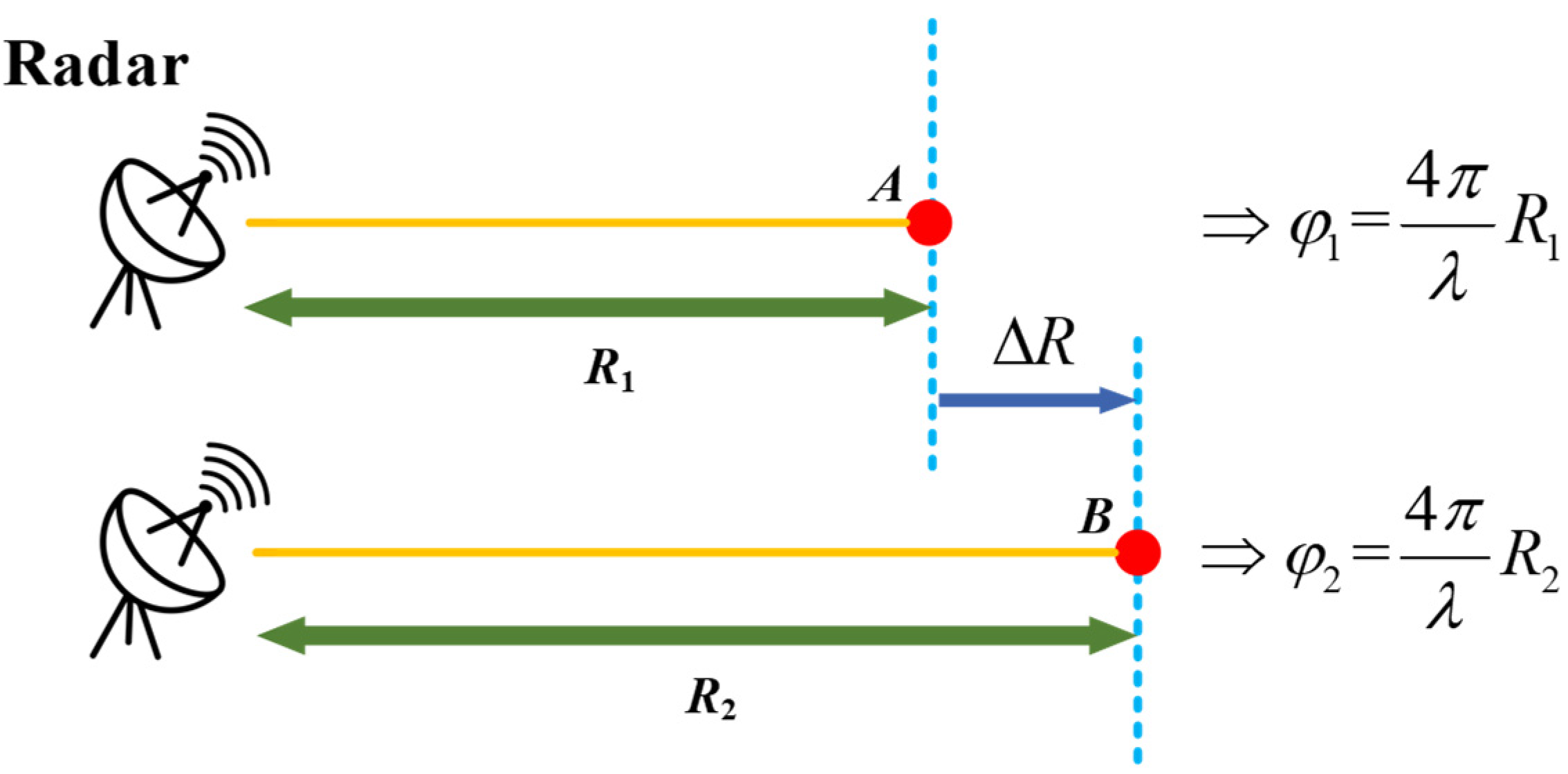
2.1. Repositioning Error Modeling

GB-SAR measurement is based on the differential interferometry technique, which utilizes the variation of the target’s phase to obtain high-precision deformation information [11]. The basic principle is shown in Figure 1. Consider a deformation target observed twice by a GB-SAR system, under ideal conditions, the interferometric phase can be expressed as:

$$\mathsf{\Delta }\phi ={\phi }_2-{\phi }_1=\frac{4\pi }{\lambda }(R_2-R_1)=\frac{4\pi }{\lambda }\mathsf{\Delta }R$$

(1)

where R₁ and R₂ are the ranges between the target and the radar during two campaigns, respectively. However, since $\mathsf{\Delta }\phi$ represents the principal value of the interferometric phase, the correct deformation estimation requires the reconstruction of the full phase value by calculating the phase ambiguity. In discontinuous mode, due to the instability of the monitoring station or lack of accurate positioning devices, the position offset of the instrument could occur during repositioning. An additional range variation is caused by the repositioning error, and $\mathsf{\Delta }R$ cannot accurately correspond to the target deformation [12].

Figure 2 shows the geometric relationship of a radar instrument. $O-xyz$ is the reference radar coordinate system, where O is the radar center, x-axis represents the direction of the synthetic aperture. After repositioning, the radar coordinate system is transformed into $O^{\prime }-x^{\prime }{y}^{\prime }{z}^{\prime }$ due to its position change.

Assuming that the coordinates of the target P and radar center O are (x_p, y_p, z_p) and (x, y, z) respectively, R can be expressed as:

$$R\left(x,y,z\right)=\sqrt{{\left(x-x_p\right)}^2+{\left(y-y_p\right)}^2+{\left(z-z_p\right)}^2}$$

(2)

The Taylor expansion of R(x, y, z) at (0, 0, 0) is:

$$\begin{array}{l}R\left(x,y,z\right)\approx {R|}_{\left(0,0,0\right)}+\left[\begin{array}{ccc}{\frac{\partial R}{\partial x}|}_{\left(0,0,0\right)}& {\frac{\partial R}{\partial y}|}_{\left(0,0,0\right)}& {\frac{\partial R}{\partial z}|}_{\left(0,0,0\right)}\end{array}\right]\left[\begin{array}{c}x\\ y\\ z\end{array}\right]+\frac{1}{2}\left[x y z\right]\left[\begin{array}{ccc}{\frac{{\partial }^{2}R}{\partial x^2}|}_{\left(0,0,0\right)}& {\frac{{\partial }^{2}R}{\partial x\partial y}|}_{\left(0,0,0\right)}& {\frac{{\partial }^{2}R}{\partial x\partial z}|}_{\left(0,0,0\right)}\\ {\frac{{\partial }^{2}R}{\partial x\partial y}|}_{\left(0,0,0\right)}& {\frac{{\partial }^{2}R}{\partial y^2}|}_{\left(0,0,0\right)}& {\frac{{\partial }^{2}R}{\partial y\partial z}|}_{\left(0,0,0\right)}\\ {\frac{{\partial }^{2}R}{\partial x\partial z}|}_{\left(0,0,0\right)}& {\frac{{\partial }^{2}R}{\partial y\partial z}|}_{\left(0,0,0\right)}& {\frac{{\partial }^{2}R}{\partial z^2}|}_{\left(0,0,0\right)}\end{array}\right]\left[\begin{array}{c}x\\ y\\ z\end{array}\right]\\ \approx R_p-\frac{x_p}{R_p}x-\frac{y_p}{R_p}y-\frac{z_p}{R_p}z+\frac{1}{2R_p^3}[(R_p^2-x_p^2)x^2+(R_p^2-y_p^2)y^2+(R_p^2-z_p^2)z^2-2x_p{y}_{p}xy-2y_p{z}_{p}yz-2x_p{z}_{p}xz]\end{array}$$

(3)

where

$$R|{}_{(0,0,0)}=R_p=\sqrt{x_p^2+y_p^2+z_p^2}$$

(4)

Since that the radar center O is located at the origin of the coordinates before the repositioning, its coordinate after the repositioning can be expressed as $({\epsilon }_x,{\epsilon }_y,{\epsilon }_z)$. Therefore, the range variation $\mathsf{\Delta }R$ from P to the radar is:

$$\begin{array}{l}\mathsf{\Delta }R=R({\epsilon }_x,{\epsilon }_y,{\epsilon }_z)-R(0,0,0)\\ \approx -\frac{x_p}{R_p}{\epsilon }_x-\frac{y_p}{R_p}{\epsilon }_y-\frac{z_p}{R_p}{\epsilon }_z+\frac{\left(R_p^2-x_p^2\right)}{2R_p^3}{\epsilon }_x^2+\frac{\left(R_p^2-y_p^2\right)}{2R_p^3}{\epsilon }_y^2+\frac{\left(R_p^2-z_p^2\right)}{2R_p^3}{\epsilon }_z^2-\frac{x_p{y}_p}{R_p^3}{\epsilon }_x{\epsilon }_y-\frac{y_p{z}_p}{R_p^3}{\epsilon }_y{\epsilon }_z-\frac{x_p{z}_p}{R_p^3}{\epsilon }_x{\epsilon }_z\end{array}$$

(5)

In discontinuous mode, it is necessary to use high-precision positioning equipment or a stable platform to guarantee that the repositioning error is as small as possible. The quadratic terms in Equation (5) can be ignored. According to Equations (1) and (5), the repositioning error phase can be simulated with a linear multi-parameter model and expressed as:

$$\mathsf{\Delta }{\phi }_{Error}\approx -\frac{4\pi }{\lambda }(\frac{x_p}{R_p}{\epsilon }_x+\frac{y_p}{R_p}{\epsilon }_y+\frac{z_p}{R_p}{\epsilon }_z)$$

(6)

where the parameters $[{\epsilon }_x,{\epsilon }_y,{\epsilon }_z]$ represent the repositioning error components, which can be estimated with the least square (LS) method. To illustrate the effects of repositioning error, the interferometric phases under different types of radar offsets are simulated. Figure 3a shows a three-dimensional (3D) topography consisting of a flat and a slope. As shown in Figure 3b, when the repositioning error is just set along the azimuth direction with ${\epsilon }_x=1 \mathrm{mm}$, the error phase $\mathsf{\Delta }{\phi }_{Error}$ changes linearly with the azimuth angle. When the repositioning error is set as ${\epsilon }_y=1 \mathrm{mm}$, whose direction is perpendicular to the azimuth, $\mathsf{\Delta }{\phi }_{Error}$ increases non-linearly with the azimuth angle, as shown in Figure 3c. For Figure 3d, there is only repositioning error component in the vertical direction ${\epsilon }_z=1 \mathrm{mm}$. It can be noted that the error phase on the flat is zero, and gradually increases with the slope height.

2.2. Simulation Comparisons

In order to reduce the influence of repositioning error on the interferometric phase, the parametric model method is commonly used. In the traditional GB-SAR algorithms, the repositioning error is explained as the incomplete repeat-pass when the radar moves to synthesize an aperture [13]. According to the observation geometry of the GB-SAR, the repositioning error can be modeled as:

$$\phi =a_0+a_1\sin \theta$$

(7)

where $\theta$ is the azimuth angle, $a_0$ and $a_1$ are two unknown parameters. For D-GBSAR, its measurement period is long and similar with the spaceborne SAR [14]. Therefore, a 2nd-order polynomial model in spaceborne SAR can be utilized to estimate the repositioning phase [15]:

$$\phi =a_0+a_1\eta +a_2\xi +a_3{\xi }^2$$

(8)

where $\eta$ and $\xi$ are the range and azimuth, respectively.

According Equation (6), an improved linear multi-parameter model is proposed and can be expressed as:

$$\phi =a_0+a_1\frac{x_p}{R_p}+a_2\frac{y_p}{R_p}+a_3\frac{z_p}{R_p}$$

(9)

The unknown parameters and error phase can be estimated based on the least square method. A numerical simulation is made to compare the compensation effects of the above three models. This paper simulates three types of topographies: flat, slope and hillside, as shown in Figure 4a. Their x-coordinate range is all from −70 m to 70 m, and y-coordinate range is all from 10 m to 100 m. For the slope, its height linearly increases with the y-coordinate and varies from 0 m to 30 m. For the hillside, the height changes irregularly with y-coordinate from 0 m to 30 m. Assuming the repositioning error along three axial directions are all 1 mm, i.e., ${\epsilon }_x={\epsilon }_y={\epsilon }_z=1 \mathrm{mm}$, Figure 4c shows the error phase maps corresponding to three terrains.

Figure 5 shows the compensation results with the three models above. With the first-order model in Equation (7), most pixels still have large residual phase errors, as shown in Figure 5a. Since the model only considers the error component along the azimuth direction, it is not suitable for the repositioning error compensation in discontinuous mode. With the second-order model in Equation (8), the compensation effects have been significantly improved compared with the first-order model. However, the second-order model doesn’t consider the error phase along the height direction. The compensation effect on the hillside is far worse than that on the flat and slope. As a conclusion, although the advantage of the former two models is that they don’t require the additional Digital Elevation Model (DEM), they cannot well eliminate the error phase if the topography is complicated. With the improved multi-parameter model in Equation (9), the error phases of all the pixels for these three terrains are close to zero.

Table 1. Statistics of residual phases.

Type	Residual Phases
	$\mathit{\phi }={\mathit{a}}_0+{\mathit{a}}_1\mathbf{sin}\mathit{\theta }$		$\mathit{\phi }={\mathit{a}}_0+{\mathit{a}}_1\mathit{\eta }+{\mathit{a}}_2\mathit{\xi }+{\mathit{a}}_3{\mathit{\xi }}^2$		$\mathit{\phi }={\mathit{a}}_0+{\mathit{a}}_1\frac{{\mathit{x}}_{\mathit{p}}}{{\mathit{R}}_{\mathit{p}}}+{\mathit{a}}_2\frac{{\mathit{y}}_{\mathit{p}}}{{\mathit{R}}_{\mathit{p}}}+{\mathit{a}}_3\frac{{\mathit{z}}_{\mathit{p}}}{{\mathit{R}}_{\mathit{p}}}$
	Max/mrad	RMSE/mrad	Max/mrad	RMSE/mrad	Max/mrad	RMSE/mrad
Flat	131.11	59.76	23.31	8.06	0.07	0.01
Slope	164.39	74.94	23.91	8.08	0.07	0.01
Hillside	211.09	86.12	48.49	10.79	0.06	0.01

shows the statistical results of the residual phases with the above three models. Under different types of terrains, the maximum residual phase and the root mean square error (RMSE) of the compensation results based on Equation (9) are much smaller than those of other two, which validates the effectiveness of the proposed model.

3. Methodology

As previously mentioned, interferometric phase is the most crucial element that determines the accuracy of deformation measurement. To select pixels suitable for phase analysis, the permanent scatterer (PS) technique is commonly applied. The PS method estimates pixels’ amplitude stability with the amplitude dispersion index (ADI). However, a limitation of the ADI approach is that it requires sufficient GB-SAR images, typically no less than 30 [16,17]. In discontinuous mode, those SAR images are coherently added to obtain a composite image in each campaign. In this case, the ADI approach is not reliable for selecting the PSs. For D-GBSAR, a general solution of PS selection is based on the coherence [18]. The coherence $\gamma$ of one pixel in an interferogram is defined as:

$$\gamma =\frac{\left|{\displaystyle \sum _{i=1}^m{\displaystyle \sum _{j=1}^{n}M(i,j)S^{*}(j,j)}}\right|}{\sqrt{{\displaystyle \sum _{i=1}^m{\displaystyle \sum _{j=1}^n{\left|M(i,j)\right|}^2{\displaystyle \sum _{i=1}^m{\displaystyle \sum _{j=1}^n{\left|S(i,j)\right|}^2}}}}}}$$

(10)

where M and S are the master and slave images, * represents complex conjugate, and (m, n) is the size of a window.

The interferometric phase of a PS can be expressed as:

$$\mathsf{\Delta }{\phi }_{PS}=\mathsf{\Delta }{\phi }_{Defo}+\mathsf{\Delta }{\phi }_{Atm}+\mathsf{\Delta }{\phi }_{\mathrm{Repo}}+\mathsf{\Delta }{\phi }_{Noise}+2k\pi$$

(11)

where $\mathsf{\Delta }{\phi }_{Defo}$ is the deformation phase, $\mathsf{\Delta }{\phi }_{Atm}$ is the atmospheric disturbance phase, $\mathsf{\Delta }{\phi }_{\mathrm{Repo}}$ is the repositioning error phase, and $\mathsf{\Delta }{\phi }_{Noise}$ is the random error phase. The interferometric phase $\mathsf{\Delta }{\phi }_{PS}$ is measured modulo $2\pi$, which is also called the wrapped phase, and $2k\pi$ is the difference between wrapped phase and absolute phase, k is an integer. The correct determination of phase ambiguity k is called phase unwrapping, which has become one of the most critical techniques in the signal processing of GB-SAR. In the following text, $\mathsf{\Delta }{\phi }_{PS}$ means the unwrapped phase.

In general, the atmosphere is homogeneous in space, $\mathsf{\Delta }{\phi }_{Atm}$ can be expressed as:

$$\mathsf{\Delta }{\phi }_{Atm}=\frac{4\pi }{\lambda }\mathsf{\Delta }N\ast R$$

(12)

where $\mathsf{\Delta }N$ represents the variation of the refractive index during two observations. Under the assumption of spatial homogeneity, $\mathsf{\Delta }{\phi }_{Atm}$ can be built as a linear phase component over the slant range:

$$\mathsf{\Delta }{\phi }_{Atm}=\frac{4\pi }{\lambda }\left(B_{1}R+B_2\right)$$

(13)

where B₁ is the linear coefficient, B₂ is an offset that can appear in the interferometric phase between two different campaigns. Together with Equation (6), for a PS with no deformation, its unwrapped phase can be modeled as:

$$\mathsf{\Delta }{\phi }_{PS}=\frac{4\pi }{\lambda }\left(A_1\frac{x_p}{R_p}+A_2\frac{y_p}{R_p}+A_3\frac{z_p}{R_p}+B_1{R}_p+B_2+e\right)$$

(14)

where [A₁, A₂, A₃, B₁, B₂] are the estimated parameters, $(x_p,y_p,z_p)$ is the 3D coordinate of the PS, R_p represents the slant range, and e is the unmodeled error phase. By estimating the polynomial parameters based on the LS method, the error phase can be compensated precisely under discontinuous mode. The equation set can be expressed as:

$$\mathsf{\Delta }\mathsf{\Phi }=X\beta +E$$

(15)

where

$$\begin{array}{l}\mathsf{\Delta }\mathsf{\Phi }=\left[\begin{array}{l}\mathsf{\Delta }{\phi }_1\\ \mathsf{\Delta }{\phi }_2\\ ⋮\\ \mathsf{\Delta }{\phi }_N\end{array}\right]X=\frac{4\pi }{\lambda }\left[\begin{array}{c}\frac{x_1}{R_1} \frac{y_1}{R_1} \frac{z_1}{R_1} R_1 1\\ \frac{x_2}{R_2} \frac{y_2}{R_2} \frac{z_2}{R_2} R_2 1\\ ⋮\\ \frac{x_N}{R_N} \frac{y_N}{R_N} \frac{z_N}{R_N} R_N 1\end{array}\right]\\ \beta =\left[\begin{array}{l}{A}_1\\ A_2\\ A_3\\ B_1\\ B_2\end{array}\right]E=\frac{4\pi }{\lambda }\left[\begin{array}{c}{e}_1\\ e_2\\ ⋮\\ e_N\end{array}\right]\end{array}$$

(16)

where $\mathsf{\Delta }\mathsf{\Phi }$ is the N × 1 vector composed with the interferometric phases of N PSs, X is the N × 5 matrix composed with the 3D coordinates and slant range of PSs, $\beta$ is the 5 × 1 vector to be estimated, and E is the N × 1 vector of error phases. The estimated parameter $\widehat{\beta }$ can be expressed as:

$$\widehat{\beta }={(X^{T}X)}^{-1}\cdot X^T\mathsf{\Delta }\mathsf{\Phi }$$

(17)

Then, the estimated phase $\mathsf{\Delta }\widehat{\mathsf{\Phi }}$ could be written as:

$$\mathsf{\Delta }\widehat{\mathsf{\Phi }}=X\widehat{\beta }$$

(18)

The difference between $\mathsf{\Delta }\mathsf{\Phi }$ and $\mathsf{\Delta }\widehat{\mathsf{\Phi }}$ is the compensated phase. Considering that there are PSs with deformations, they could affect the estimation accuracy. In order to achieve a better estimation, an iterative process is commonly applied to filter out PSs with deformations [19]. The judgement can be fulfilled as Equation (13), and ${\phi }_T$ is typically set within 0.1 to 0.2 rad. Then the selected PSs are prepared for the next estimation.

$$\left|\mathsf{\Delta }\mathsf{\Phi }-\mathsf{\Delta }\widehat{\mathsf{\Phi }}\right|<{\phi }_T$$

(19)

The iterative process is terminated until all of the remaining PSs can meet the conditions of Equation (13).

In scenes with steep topographic variations, the refractivity index N could change in the space domain, the assumption of spatial homogeneity no longer applies [20]. In this case, $\mathsf{\Delta }{\phi }_{Atm}$ can be expressed as:

$$\mathsf{\Delta }{\phi }_{Atm}=\frac{4\pi }{\lambda }\left(\mathsf{\Delta }N\cdot R-\mathsf{\Delta }N\cdot \alpha \cdot \frac{R\cdot \mathsf{\Delta }h}{2}\right)$$

(20)

where $\mathsf{\Delta }h$ denotes the height difference between the radar and target, $\alpha$ is the inverse of a height scale factor. A range-height model, over mountainous regions is proposed:

$$\mathsf{\Delta }{\phi }_{Atm}=\frac{4\pi }{\lambda }\left(B_{1}R+B_{2}R\cdot \mathsf{\Delta }h+B_3\right)$$

(21)

Comparing Equations (7) and (15), there is an additional term with $R\cdot \mathsf{\Delta }h$ in the range-height model, which requires the DEM information of the experimental scenario before measurement.

4. Experimental Results

4.1. First Case: Urban Area

4.1.1. Experiment Information

Figure 6 shows the photo of the ground-based multiple-input-multiple-output (GB-MIMO) radar, which uses 16 transmitting antennas and 16 receiving antennas to synthesize an equivalent linear array with 256 phase centers [21]. The GB-MIMO radar works at the Ku-band, and its transmitted signal is frequency-modulated continuous wave.

Table 2. System parameters of the GB-MIMO radar.

Parameter	Value
Carrier Frequency	16.2 GHz
Wavelength	18.5 mm
Synthetic Aperture	1.18 m
Bandwidth	1 GHz
Range Resolution	0.15 m
Azimuth Angle Resolution	7.81 mrad

shows the specific parameters of the GB-MIMO system. Note that the cross-range resolution is not constant, ranging from 0.39 m at the near range of 50 m up to 7.81m at the far range of 1000 m.

Figure 7a shows the experimental scenario, which is an outdoor lawn located in the Chongqing Innovation Center of Beijing Institute of Technology. The GB-MIMO radar is set on an observation platform. Two corner reflectors (CRs) are utilized as reference points. The red circles mark the CRs, and the yellow blocks show enlarge images. Figure 7b shows the radar image, which could be regarded as a signal-to-noise ratio (SNR) map. Pixels with SNR above 60dB correspond to streetlights, seats, and buildings.

Discontinuous monitoring mode is mainly applied for creepy landslides. For each campaign, only several GB-SAR images are acquired within a short time, and no deformations would occur. Then after several weeks or months, another monitoring campaign is taken, and small deformation of several millimeters might occur. To simulate the deformation phenomenon of discontinuous monitoring as accurately as possible, an equivalent validation experiment was carried out.

The GB-MIMO radar was used to monitor the scenario on 10 December 2020, and the monitoring time lasted from 14:41 to 16:41. The radar system acquired 93 radar images. During the experiment, the radar was moved six times, and it could be regarded as a discontinuous monitoring experiment with seven monitoring campaigns. A total station was used to measure the radar position, as shown in

Table 3. Offsets of the radar center.

Serial	Offsets
	${\mathit{\epsilon }}_{\mathit{x}} \left(\mathbf{mm}\right)$	${\mathit{\epsilon }}_{\mathit{y}} \left(\mathbf{mm}\right)$
No.1	0.11	0.32
No.2	−6.28	0.32
No.3	−2.62	−0.15
No.4	0.17	−1.31
No.5	−0.46	5.16
No.6	−3.48	4.75

. Since the instrument wasn’t moved in the vertical direction, the error component in height wasn’t considered, i.e., ${\epsilon }_z=0 \mathrm{mm}$.

Every two adjacent radar images of the 93 images were taken as an interferometric pair, and 92 interferograms were generated. Figure 8 shows the interferometric phases of CR₁ and CR₂. The horizontal axis represents the moments when radar images were acquired. The red lines mark the moments when the radar was moved, and the interferometric phases of both CRs vary significantly. In contrast, during the period of stable monitoring, their interferometric phases are close to zero. Every time the MIMO radar was moved, multiple radar images were acquired and they were coherently added to obtain a composite image. Seven composite images were acquired in this experiment, denoted as M₁~M₇.

4.1.2. Model Validation

As shown in Figure 2, the synthetic aperture may be rotated after repositioning, which could cause variations in the targets’ azimuth angles. The co-registration step is fundamental in interferogram generation. The process of image co-registration involves image matching, transformation estimation, and image resampling [22]. The shift estimation can be performed by using the incoherent correlation of the squared amplitudes of the two images. For GB-SAR image co-registration, an oversampling factor of 16 is typically utilized to achieve the accuracy of 1/10 pixels. After image co-registration, two adjacent composite images are taken as an interferometric pair, 6 phase interferograms can be obtained, denoted as IM₁~IM₆. Since the experimental scenario is flat and stable, the interferometric phases mainly contain repositioning error and atmospheric components.

Using the total station to obtain the 3D coordinates of both CRs, combining with the radar offsets in Table 3, the theoretical values of repositioning error phases of both CRs are obtained with Equation (6), as shown with the red dotted lines in Figure 9. The blue solid lines show the measured curves of interferometric phases of both CRs with IM₁~IM₆. Due to the millimeter-level positioning error of the total station, there are slight differences between these curves, but it could still prove that the proposed method can model the repositioning error precisely.

4.1.3. Error Compensation

Consider M_i as the master image and M_i+1 as the slave image (i = 1, 2, …, 6), 6 coherence maps are acquired, the average coherence map is shown in Figure 10a. As mentioned in Section 3, the coherence method is used to select PSs in discontinuous mode. Set the coherence threshold as 0.98 and the SNR threshold as 30 dB, 51,387 PSs are obtained, which are shown in Figure 10b. The pixels corresponding to both CRs and most building structures are selected as PSs.

Take IM₁ as an example for phase analysis, the phase unwrapping is performed based on the Minimum Cost Flow method [23]. The unwrapped phase map of PSs is shown in Figure 11a. The interferometric phases of most PSs deviate from 0 rad due to the repositioning error. The topography of experimental scenario is mainly flat, so the linear range model of the atmospheric phase component in Equation (13) is utilized. Since that the radar was not moved in the height direction, the phase model in Equation (14) can be simplified as:

$$\mathsf{\Delta }{\phi }_{PS}=\frac{4\pi }{\lambda }\left(A_1\frac{x_p}{R_p}+A_2\frac{y_p}{R_p}+B_1{R}_p+B_2+e\right)$$

(22)

As mentioned in Section 3, the repositioning error and the atmospheric phase of these PSs are jointly compensated by the iterative LS method. Figure 11b shows histograms of the unwrapped phases and estimated phases. Figure 11c shows the compensated phase map. Figure 11d shows the phase distribution curve after the error compensation. For most PSs, their compensated phases slightly deviate from 0 rad, which proves that the error phases have been well compensated with the proposed method.

Figure 12 shows the phase curves of both CRs before and after compensation.

Table 4. Statistical results of residual phases for both CRs.

Serial	Residual Phases
	CR1		CR2
	Max/rad	σ/rad	Max/rad	σ/rad
Before Compensation	3.11	2.48	2.98	2.27
After Compensation	0.11	0.05	0.17	0.09

shows the statistics of the maximum values and standard deviation σ of the residual phases for both CRs before and after the error compensation. σ is about 0.1 rad after compensation. For the Ku-band GB-MIMO radar, the corresponding deformation is 0.14 mm, which meets the requirements of sub-millimeter measuremen.

4.2. Second Case: Mountainous Area

4.2.1. Experiment Information

Mayan area (N29°35′40.46″, E108°25′45.77″) in Pengshui County of Chongqing City is a dangerous rock mass. A GB-MIMO radar was applied to monitor the mountainous area in discontinuous mode, two campaigns of data collection were performed in 24 September and 1 November 2020. Between different campaigns, the radar was reinstalled onto the observation platform, which caused repositioning errors at mm level.

Figure 13a shows the photo of the experimental scenario, where the monitoring scenario is marked in red box. Figure 13b is the signal-to-noise (SNR) map of the scenario. Those pixels with SNR above 30 dB correspond to the bare rocky slope. The difference of height between the radar and experimental scenario is shown in Figure 13c.

4.2.2. Experimental Results

The error compensation was carried out based on PS technique, the coherence threshold is set as 0.8 and the SNR threshold is 30 dB. Figure 14c,d are the interferometric phase maps of PSs before and after phase unwrapping. For the unwrapped phase map in Figure 14d, a non-linear variation over range is shown. Figure 13c indicates that the height difference between the radar and observation scene varies from −200 to 900m, the range-height model in Equation (21) is utilized as atmospheric phase component.

Based on PSs, the first-order, second-order and improved multi-parameter models of the repositioning error phase in Section 2.2 are utilized. The unwrapped interferometric phase of PS can be expressed as Model A, B, and C respectively:

$$\begin{array}{l}Model A: \mathsf{\Delta }{\phi }_{PS}=\frac{4\pi }{\lambda }\left(A_1\sin {\theta }_p+B_1{R}_p+B_{2}R\cdot \mathsf{\Delta }h+B_3+e\right)\\ Model B: \mathsf{\Delta }{\phi }_{PS}=\frac{4\pi }{\lambda }\left(A_1\eta +A_2\xi +A_3{\xi }^2+B_1{R}_p+B_{2}R\cdot \mathsf{\Delta }h+B_3+e\right)\\ Model C: \mathsf{\Delta }{\phi }_{PS}=\frac{4\pi }{\lambda }\left(A_1\frac{x_p}{R_p}+A_2\frac{y_p}{R_p}+A_3\frac{z_p}{R_p}+B_1{R}_p+B_{2}R\cdot \mathsf{\Delta }h+B_3+e\right)\end{array}$$

(23)

The corresponding phase scatter diagrams are SD_A, SD_B, SD_C, as shown in Figure 15a,c,e. Obviously, the phase scatter could be better simulated with Model C. The compensation results are CIM_A, CIM_B, CIM_C, as shown in Figure 15b,d,f. Figure 15g shows the phase distribution curves of the residual phases under different models. Compared with the improved method, there are a large number of PSs deviate from 0 rad with Model A and B. According to the on-site investigation, there were no obvious deformations for the high and steep rocky slope during the experiment. We could conclude that the best compensation performance could be achieved with the improved multi-parameter model. However, the red circle in Figure 15f marks a deformation area, where the negative deformations denote the direction away from the radar.

With the iterative LS method proposed in Section 3, the repositioning error components are ${\epsilon }_x=-3.17 \mathrm{mm}$, ${\epsilon }_y=0.93 \mathrm{mm}$, ${\epsilon }_z=-1.40 \mathrm{mm}$, respectively. The cumulative deformation during the entire measurement period is matched with the 3D topography, as shown in Figure 16, where the red box indicates the location of the radar.

5. Discussion

Discontinuous GB-SAR monitoring is suitable for creep-type landslides. However, as shown in Figure 2, the offset of the radar center may cause the loss of coherence and reduce the accuracy of deformation monitoring, which is called the repositioning error. Generally, parametric modeling is applied for error compensation. In the conventional GB-SAR algorithm, the first-order and second-order models are commonly used to estimate the repositioning error. However, for the scenes with steep topographic variations, the above two models cannot well eliminate the error phase and severe residual phases are remaining.

A linear multi-parameter model based on the Taylor expansion of a ternary function is proposed to estimate the repositioning error phase. Firstly, the analysis based on three simulated topographies is made in Section 2.2. The compensation results shown in Figure 5 and Table 1 indicate that the repositioning error phases of all the pixels for three kinds of terrains are close to zero with the improved multi-parameter model. In Section 3, the PS technique is applied to jointly compensate the repositioning error and atmospheric disturbance. Two cases with GB-MIMO radar in discontinuous mode have been described in Section 4.

• Case 1: An equivalent experiment of discontinuous mode is made by slightly moving the radar. The error compensation results are shown in Figure 11. Two corner reflectors are set to validate the effectiveness of the proposed model, as shown in Figure 12. The standard deviation of residual phases for both CRs is about 0.1 rad, which corresponds to 0.14 mm in Ku band, and can satisfy the requirement of sub-millimeter measurement.
• Case 2: The improved method is applied to process the measured data of a mountainous area. Comparisons of the first-order, second-order and proposed model are shown in Figure 15. There are a large number of PSs deviate from 0 rad with conventional models, and the best compensation performance could be achieved with the improved multi-parameter model. Figure 15f shows the compensated curves, which proves that the error phase components can be better compensated with the improved method.

6. Conclusions

Aiming at solving the repositioning error of GB-SAR in discontinuous mode, this paper proposes an error compensation method based on multi-parameter modeling. Under D-GBSAR mode, the radar instrument needs to be installed and disassembled repeatedly, which leads to the repositioning error. Based on the Taylor expansion of a ternary function, the repositioning error is decomposed, and can be simulated with a linear multi-parameter model. Quantitative comparisons with two common first-order and second-order models under three types of simulated topographies are firstly made to validate the effectiveness of this model. Then this paper proposes to jointly compensate the repositioning error and atmospheric disturbance phases based on the PS technique. By building a linear equation set with enough PSs and iteratively solving it, those model parameters could be estimated. Two examples of GB-MIMO radar deformation monitoring are made in discontinuous mode. By analyzing the results of CRs and PSs, the improved method can effectively compensate for the error phase, and benefit, ensuring the sub-millimeter measurement accuracy of GB-SAR.

References

1. Zhao, C.; Lu, Z. Remote Sensing of Landslides: A Review. Remote Sens. 2018, 10, 279. [Google Scholar] [CrossRef] [Green Version]
2. Colesanti, C.; Wasowski, J. Investigating landslides with space-borne Synthetic Aperture Radar (SAR) interferometry. Eng. Geol. 2006, 88, 173–199. [Google Scholar] [CrossRef]
3. Iglesias, R.; Aguasca, A.; Fabregas, X.; Mallorqui, J.J.; Monells, D.; Lopez-Martinez, C.; Pipia, L. Ground-Based Polarimetric SAR Interferometry for the Monitoring of Terrain Displacement Phenomena–Part II: Applications. IEEE J. Sel. Top. Appl. Earth Obs. Remote Sens. 2014, 8, 994–1007. [Google Scholar] [CrossRef] [Green Version]
4. Pieraccini, M.; Miccinesi, L. Ground-Based Radar Interferometry: A Bibliographic Review. Remote Sens. 2019, 11, 1029. [Google Scholar] [CrossRef] [Green Version]
5. Wang, Y.; Hong, W.; Zhang, Y.; Lin, Y.; Li, Y.; Bai, Z.; Zhang, Q.; Lv, S.; Liu, H.; Song, Y. Ground-Based Differential Interferometry SAR: A Review. IEEE Geosci. Remote Sens. Mag. 2020, 8, 43–70. [Google Scholar] [CrossRef]
6. Monserrat, O.; Crosetto, M.; Luzi, G. A review of ground-based SAR interferometry for deformation measurement. ISPRS J. Photogramm. Remote Sens. 2014, 93, 40–48. [Google Scholar] [CrossRef] [Green Version]
7. Crosetto, M.; Monserrat, O.; Luzi, G.; Cuevas-González, M.; Devanthéry, N. Discontinuous GBSAR deformation monitoring. ISPRS J. Photogramm. Remote Sens. 2014, 93, 136–141. [Google Scholar] [CrossRef] [Green Version]
8. Li, Z.; Wang, J.; Li, L.; Wang, L.; Liang, R.Y. A case study integrating numerical simulation and GB-InSAR monitoring to analyze flexural toppling of an anti-dip slope in Fushun open pit. Eng. Geol. 2015, 197, 20–32. [Google Scholar] [CrossRef] [Green Version]
9. Pan, X.; Xu, Y.; Xing, C.; Wang, P.; Zhong, L. Study of a GB-SAR Rail Error Correction Method Based on an Incident Angle Model. IEEE Trans. Geosci. Remote Sens. 2019, 58, 510–518. [Google Scholar] [CrossRef]
10. Barla, M.; Antolini, F.; Bertolo, D.; Thuegaz, P.; D’Aria, D.; Amoroso, G. Remote monitoring of the Comba Citrin landslide using discontinuous GBInSAR campaigns. Eng. Geol. 2017, 222, 111–123. [Google Scholar] [CrossRef]
11. Wang, P.; Xing, C.; Pan, X. Reservoir Dam Surface Deformation Monitoring by Differential GB-InSAR Based on Image Subsets. Sensors 2020, 20, 396. [Google Scholar] [CrossRef] [PubMed] [Green Version]
12. Hu, C.; Zhu, M.; Zeng, T.; Tian, W.; Mao, C. High-precision deformation monitoring algorithm for GBSAR system: Rail determination phase error compensation. Sci. China Inf. Sci. 2016, 59, 204–219. [Google Scholar] [CrossRef] [Green Version]
13. Luzi, G.; Pieraccini, M.; Mecatti, D.; Noferini, L.; Guidi, G.; Moia, F.; Atzeni, C. Ground-based radar interferometry for landslides monitoring: Atmospheric and instrumental decorrelation sources on experimental data. IEEE Trans. Geosci. Remote Sens. 2004, 42, 2454–2466. [Google Scholar] [CrossRef]
14. Shirzaei, M.; Walter, T. Estimating the Effect of Satellite Orbital Error Using Wavelet-Based Robust Regression Applied to InSAR Deformation Data. IEEE Trans. Geosci. Remote Sens. 2011, 49, 4600–4605. [Google Scholar] [CrossRef]
15. Wang, Z.; Li, Z.; Mills, J. Modelling of instrument repositioning errors in discontinuous Multi-Campaign Ground-Based SAR (MC-GBSAR) deformation monitoring. ISPRS J. Photogramm. Remote Sens. 2019, 157, 26–40. [Google Scholar] [CrossRef]
16. Hu, C.; Deng, Y.; Tian, W.; Wang, J. A PS processing framework for long-term and real-time GB-SAR monitoring. Int. J. Remote Sens. 2019, 40, 6298–6314. [Google Scholar] [CrossRef]
17. Tofani, V.; Raspini, F.; Catani, F.; Casagli, N. Persistent Scatterer Interferometry (PSI) Technique for Landslide Characterization and Monitoring. Remote Sens. 2013, 5, 1045–1065. [Google Scholar] [CrossRef] [Green Version]
18. Zhao, F.; Mallorqui, J.J. A Temporal Phase Coherence Estimation Algorithm and Its Application on DInSAR Pixel Selection. IEEE Trans. Geosci. Remote Sens. 2019, 57, 8350–8361. [Google Scholar] [CrossRef] [Green Version]
19. Deng, Y.; Hu, C.; Tian, W.; Zhao, Z. A Grid Partition Method for Atmospheric Phase Compensation in GB-SAR. IEEE Trans. Geosci. Remote Sens. 2021, 1–13. [Google Scholar] [CrossRef]
20. Zhao, X.; Lan, H.; Li, L.; Zhang, Y.; Zhou, C. A Multiple-Regression Model Considering Deformation Information for Atmospheric Phase Screen Compensation in Ground-Based SAR. IEEE Trans. Geosci. Remote Sens. 2019, 58, 777–789. [Google Scholar] [CrossRef]
21. Deng, Y.; Hu, C.; Tian, W.; Zhao, Z. 3-D Deformation Measurement Based on Three GB-MIMO Radar Systems: Experimental Verification and Accuracy Analysis. IEEE Geosci. Remote Sens. Lett. 2020, 1–5. [Google Scholar] [CrossRef]
22. Monserrat, O. Deformation measurement and monitoring with GB-SAR. Ph.D. Thesis, Polytechnic University of Catalonia, Barcelona, Spain, 2012. [Google Scholar]
23. Costantini, M. A novel phase unwrapping method based on network programming. IEEE Trans. Geosci. Remote Sens. 1998, 36, 813–821. [Google Scholar] [CrossRef]
Figure 1. Diagram of deformation measurement.
Remotesensing 13 02461 g001
Figure 2. Ground-based synthetic aperture radar (GB-SAR) geometry.
Remotesensing 13 02461 g002
Figure 3. Simulation of repositioning errors: (a) Topography; (b) ε x = 1   mm ,   ε y = 0 ,   ε z = 0 ; (c) ε x = 0 ,   ε y = 1   mm ,   ε z = 0 ; (d) ε x = 0 ,   ε y = 0 ,   ε z = 1   mm .
Remotesensing 13 02461 g003
Figure 4. Simulation of repositioning errors with three different kinds of topographies ( ε x = ε y = ε z = 1   mm ): (a) Topographies; (b) Elevations; (c) Repositioning error phase maps.
Remotesensing 13 02461 g004
Figure 5. Compensation results of repositioning error phase with three different models ( ε x = ε y = ε z = 1   mm ): (a) φ = a 0 + a 1 sin θ ; (b) φ = a 0 + a 1 η + a 2 ξ + a 3 ξ 2 ; (c) φ = a 0 + a 1 x p R p + a 2 y p R p + a 3 z p R p .
Remotesensing 13 02461 g005
Figure 6. Photo of the ground-based multiple-input multiple-output (GB-MIMO) radar.
Remotesensing 13 02461 g006
Figure 7. (a) Experimental scenario; (b) Signal-to-noise (SNR) map.
Remotesensing 13 02461 g007
Figure 8. Interferometric phases of both corner reflectors (CRs): (a) CR1; (b) CR2.
Remotesensing 13 02461 g008
Figure 9. Comparison of theoretical value and experimental data from both two CRs: (a) CR1; (b) CR2.
Remotesensing 13 02461 g009
Figure 10. (a) Average coherence map; (b) Permanent scatterer (PS) selection result.
Remotesensing 13 02461 g010
Figure 11. Results of error phase compensation in IM1: (a) Unwrapped phase map (Before compensation); (b) Corresponding histograms; (c) Compensated phase map; (d) Phase distribution curve.
Remotesensing 13 02461 g011
Figure 12. Compensation results of CRs error phases: (a) CR1; (b) CR2.
Remotesensing 13 02461 g012
Figure 13. Experimental scenario: (a) Photo; (b) SNR map; (c) Elevations in radar coordinates.
Remotesensing 13 02461 g013
Figure 14. Results of PS selection: (a) Interferometric phase map; (b) Coherence map; (c) Wrapped phases of PSs; (d) Unwrapped phases of PSs.
Remotesensing 13 02461 g014aRemotesensing 13 02461 g014b
Figure 15. Phase scatter diagrams: (a) SDA; (c) SDB; (e) SDC. Compensation results: (b) CIMA; (d) CIMB; (f) CIMC. Comparison of different models: (g) Phase distribution curves of residual phases.
Remotesensing 13 02461 g015aRemotesensing 13 02461 g015b
Figure 16. Cumulative deformation map.
Remotesensing 13 02461 g016