Article

HOLBP: Remote Sensing Image Registration Based on Histogram of Oriented Local Binary Pattern Descriptor

1
School of Mathematics, Northwest University, Xi’an 710127, China
2
School of Computer Science, Shaanxi Normal University, Xi’an 710119, China
3
Department of Computing Science, University of Alberta, Edmonton, AB T6G 2E8, Canada
*
Author to whom correspondence should be addressed.
Remote Sens. 2021, 13(12), 2328; https://doi.org/10.3390/rs13122328
Submission received: 8 April 2021 / Revised: 27 May 2021 / Accepted: 3 June 2021 / Published: 14 June 2021

Abstract

:
Image registration has always been an important research topic. This paper proposes a novel method of constructing descriptors called the histogram of oriented local binary pattern descriptor (HOLBP) for fast and robust matching. There are three new components in our algorithm. First, we redefined the gradient and angle calculation template to make it more sensitive to edge information. Second, we proposed a new construction method of the HOLBP descriptor and improved the traditional local binary pattern (LBP) computation template. Third, the principle of uniform rotation-invariant LBP was applied to add 10-dimensional gradient direction information to form a 138-dimension HOLBP descriptor vector. The experimental results showed that our method is very stable in terms of accuracy and computational time for different test images.

Graphical Abstract

1. Introduction

The process of matching and superimposing two or more images extracted for different times, sensors (imaging equipment), or conditions (e.g., weather, illuminance, and camera position and angle) is called image registration [1]. In some fields, such as remote sensing data analysis, computer vision [2], image fusion [3], image segmentation [4], and image clustering [5], it has been shown to have a wide range of applications [6,7]. The general gray level-based normalized product correlation method cannot handle scale changes, while phase correlation registration based on the frequency domain can only obtain the translation parameters of the image [1,8].
Although mutual information (MI) can be used as a registration metric for multi-sensor images, the computational complexity of mutual information is very high [9,10].
To register real-time images with reference images, it is necessary to extract features from the acquired images and establish a corresponding relationship with the extracted feature information [9,11]. The features consist of points, lines, curves, and surfaces, including corners, straight lines, edges, templates, regions, and contours. By solving the feature correspondence relationship, the transformation between the real-time image and the reference image (usually a transformation matrix) is obtained, and finally, the real-time image is transformed into the required form by selecting different modes according to the geometric relationships [12].
In recent years, Ye et al. [13,14] proposed the histogram of orientated phase congruency (HOPC) and developed the channel features of orientated gradients (CFOG) for multimodal remote sensing image registration. Wu et al. [15] proposed the fast sample consensus (FSC) algorithm, and an iterative method to increase the number of correct correspondences. Ma et al. [16,17,18,19] proposed robust feature matching of remote sensing images via vector field consensus and a locality preserving technique to remove mismatches.
Among existing image registration algorithms, those based on features with points occupy a central position, e.g., Harris corner detection and scale-invariant feature transform (SIFT) [20]. However, when the SIFT algorithm is applied to remote sensing images, it is affected by terrain, illumination, and other factors, resulting in many key point mismatches [21]. Zhang et al. [8] presented an improved SIFT method for accuracy and robustness based on local affine constraints with a circle descriptor. Chang et al. [22] proposed a method based on a modified SIFT and feature slope grouping to improve the feature matching and the efficiency of the algorithm. However, this also increases the number of mismatched points in the feature set and leads to reduced registration accuracy.
In order to solve the problems of SIFT in remote sensing images, the main contributions of our paper are:
  • Redefinition of Gradient and Orientation:
    Based on the Laplacian and Sobel operators, we improved the edge information representation to improve robustness.
  • Constructing descriptor:
    Based on the local binary pattern (LBP) operator, we proposed a new descriptor, histogram of oriented local binary pattern descriptor (HOLBP), which constructs histograms using the gradient direction of feature points and the LBP value. The texture information of an image and the rotation invariance of the descriptor were preserved as much as possible. We applied the principle of uniform rotation-invariant LBP [23] to add 10-dimensional gradient direction information, based on a 128-dimension descriptor of HOLBP, to enhance matching. This increased the abundance of the description information with eight directions.
  • Matching:
    After the coordinates of the matched points were initially obtained, we used rotation-invariant direction information for selection to ameliorate the instability of the Random Sample Consensus (RANSAC) algorithm.

2. Methods

In this section, we introduce the remote sensing image registration method in four subsections. The main content is organized as follows: redefinition of image gradient and its use to determine the main direction of feature points; the composition of the HOLBP descriptor; and specific operations in matching assignments.

2.1. Scale-Space Pyramid and Key Point Localization

This step exploits the Gaussian pyramid to construct the scale space, which is the same as the SIFT algorithm [20].

2.2. Gradient and Orientation Assignment

The algorithm of spatial domain processing relies on the relevant calculation of image pixels. Nevertheless, a real image often contains noise from uncertain sources, which leads to errors in gradient and angle information calculations. In order to extract the edge features of images more accurately, we redefined the calculation template of gradient and gradient direction based on the Laplacian and Sobel operators. The new template can smooth noise and provide more accurate edge direction information. This can be expressed as:
G x , σ = h 1 I ( x , y ) G y , σ = h 1 T I ( x , y )
where h 1 is the convolution kernel, i.e., h 1 = 1 1 1 1 4 3 1 1 1 , h 1 T is the transpose of h 1 , is the convolution operator, I ( x , y ) is the input image, σ is the scale in Gaussian scale space, and G x , σ and G y , σ represent the derivatives in the horizontal and vertical directions, respectively. Thus, the gradient magnitude and gradient direction are:
G ( x , y , σ ) = ( G x , σ ) 2 + ( G y , σ ) 2 θ ( x , y , σ ) = arctan ( G y , σ / G x , σ )
where G ( x , y , σ ) and θ ( x , y , σ ) represent the gradient magnitude and direction, respectively.
Here, we used a simple test image to illustrate the difference between the new template and the ordinary Sobel and Laplacian operators. Figure 1 shows that our new gradient template could keep the original shape of the rectangle and highlight the edges at the same time when image corrupted with multiplicative noise which simulates the real processing of registration.

2.3. Construct HOLBP Descriptor

The original SIFT descriptor is constructed based on the gradient information; however, it ignores complex image contours or textures. Although Lowe [20] suggested that the normalization of descriptors could eliminate the effect of illumination, the results of the registration experiments were not satisfactory. We have performed many experiments, which indicate that the gradient information itself cannot fully represent the image texture information. Consequently, we proposed the novel HOLBP descriptor, which consists of two parts to address the above-mentioned problem.

2.3.1. HOLBP

After rotating the position and direction of the image gradient in a neighborhood near a feature point into the main direction, SIFT takes the feature point as the center to select an area of m σ B p × m σ B p size in the rotated image. It is divided into B p × B p subregions at equal intervals, which are pixels. Here, m = 3 , B p = 4 , and σ is the scale value of the feature point.
The LBP operator [23] is derived in a 3 × 3 window, with the central pixel of the window as the threshold. The gray values of the adjacent 8 pixels are compared with it; if the surrounding pixel value is greater than the central pixel value, the position of the pixel is marked as 1; otherwise, it is marked as 0. In this way, an 8-bit binary number can be generated for comparison in this window and can be converted into a total of 256 decimal numbers. The calculation of the LBP value is given by the following formula:
L B P ( x r , y r ) = p = 0 P 1 2 p s ( i p i r )
where s ( ) is a sign function, i.e., s ( x ) = 1 i f       x 0 0 o t h e r w i s e , ( x r , y r ) is the center pixel, i r is the grayscale value, i p represents gray values of adjacent pixels, and P is the number of sample points. In this article, P = 8 .
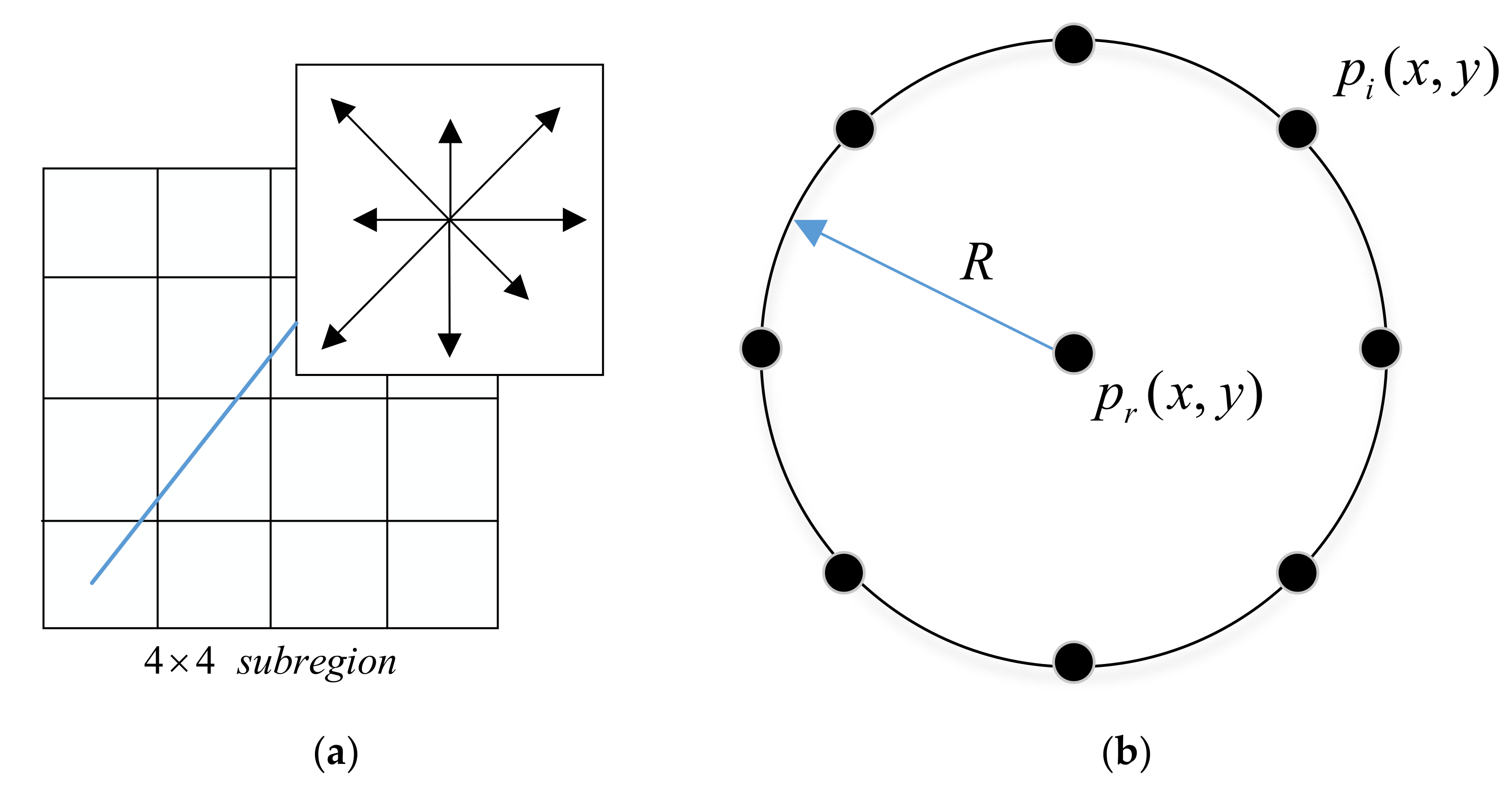
The proposed HOLBP descriptor is based on the LBP operator, which calculates the LBP histogram of each subregion in eight directions centered on the feature points, and draws the accumulated value of each gradient direction to form a seed point. At this time, the direction of LBP for each subregion divides 0° to 360° into 8 ranges, with each range being 45° so that every seed point has 8 directions of LBP intensity information, as shown in Figure 2a. Considering B p × B p subregions at equal intervals, there are a total of 4 × 4 × 8 = 128 values.
Note that the LBP calculated this way cannot be directly applied in calculations, due to the 256 unconverted values causing a Euclidean distance mismatch. Thus, we ameliorate the traditional LBP computation by adding an 8-domain Laplacian template operator to make it more efficacious. The convolution formulae are:
L B P x , σ = h 2 L ( x , y ) L B P y , σ = h 2 T L ( x , y )
where h 2 is the convolution kernel, i.e., h 2 = 1 1 1 1 8 1 1 1 1 , h 2 T is the transpose of h 2 , is the convolution operator, L ( x , y ) is the LBP image of subregions, σ is the scale in Gaussian scale space, and L B P x , σ and L B P y , σ represent the derivatives in the horizontal and vertical directions, respectively. It is easy to obtain the improved LBP magnitude:
L B P ( x , y , σ ) = ( L B P x , σ ) 2 + ( L B P y , σ ) 2 = 2 L B P x , σ = 2 L B P y , σ
where L B P ( x , y , σ ) represents the improved LBP magnitude.
There are two reasons why we calculate LBP this way. One is that it will cause Euclidean distance matching errors if we directly use numerical values to generate the histogram. The other is that a convolution operation will not change the LBP image in the x or y direction but smooth and enhance the texture of the image to a certain extent.
For our method, the gradient itself is also the rate of change of the gray value, which is similar to the LBP calculation. Thus, we form a 128-dimensional HOLBP descriptor filling the gap in the texture information for the SIFT descriptor, which is denoted as H O L B P 128 .

2.3.2. Riu-Direction

The reason why SIFT can have the property of rotation invariance is that in the descriptor histogram, eight directions are obtained to distinguish the magnitude of the gradient. Nevertheless, these directions cannot represent the direction variations of all feature points, as there will be mismatching in the matching task. The proposed HOLBP descriptor adds 10-dimensional gradient direction information to enhance the matching and rotation invariance.
Before the next step, we need to mention the concept of Uniform Rotation-Invariant LBP (Riu-LBP). Ojala et al. [23] improved the LBP operator to extend a 3 × 3 neighborhood to any neighborhood, replacing the square neighborhood, and they obtained a series of LBP feature values by rotating the resulting LBP features, as shown in Figure 2b. For eight sampling points, there are 36 unique rotation-invariant binary patterns, but more pattern types make the amount of data too large and the histogram too sparse. Ojala et al. thus proposed a “uniform pattern” that reduced the dimensionality of 36 rotation-invariant binary patterns to 10.
The Riu-LBP is achieved by simply counting the number of jumps in the basic LBP code for uniform patterns, or setting P + 1 for non-uniform patterns. Inspired by this approach, our method describes the gradient angle information in the subregion from the Riu direction:
D I R ( P , R ) = p = 0 P 1 2 p s ( a ( d p ) a ( d r ) ) D I R ( P , R ) R i = min { R O R ( D I R ( P , R ) , i ) | i = 0 , 1 , , P 1 } D I R ( P , R ) R i u = p = 0 P 1 s ( a ( d p ) a ( d r ) ) ,   f o r   u n i f o r m   p a t t e r n s P + 1 , o t h e r w i s e
where d r is the center pixel, d p is the adjacent pixel, a is the gradient direction of a pixel, and R O R ( x , i ) performs a circular bit-wise right shift on the P-bit number x, i times. R is the radius of the circular window, P is number of sample points, and s is the sign function. For the detailed description of the formula and the mode of uniform pattern, please refer to paper [23]. In this paper, we utilized the above formula to calculate the angle change information within the circular domain of the feature point. This model makes up for the defect of incomplete angle description information caused by only dividing eight directions when generating descriptors.
Thus, we obtain the 10-dimensional Riu gradient direction feature:
D I R i = D I R 8 , 1 R i u
where the maximum value in D I R i indicates the most representative angle-jump mode near the feature point. Combining H O L B P i with D I R i , we construct a new 138-dimensions feature vector:
( H O L B P . D I R ) i = [ H O L B P i       D I R i ]
where i = 1 , 2 , , n , and n represents the number of feature points. We obtain a new descriptor within the sampling range of each feature point (the sampling range is explained in Section 2.3.1). The eigenvector expression of an image with n key points can be denoted by:
H O L B P 138 = [ ( H O L B P . D I R ) 1 ( H O L B P . D I R ) 2 ( H O L B P . D I R ) n ] T
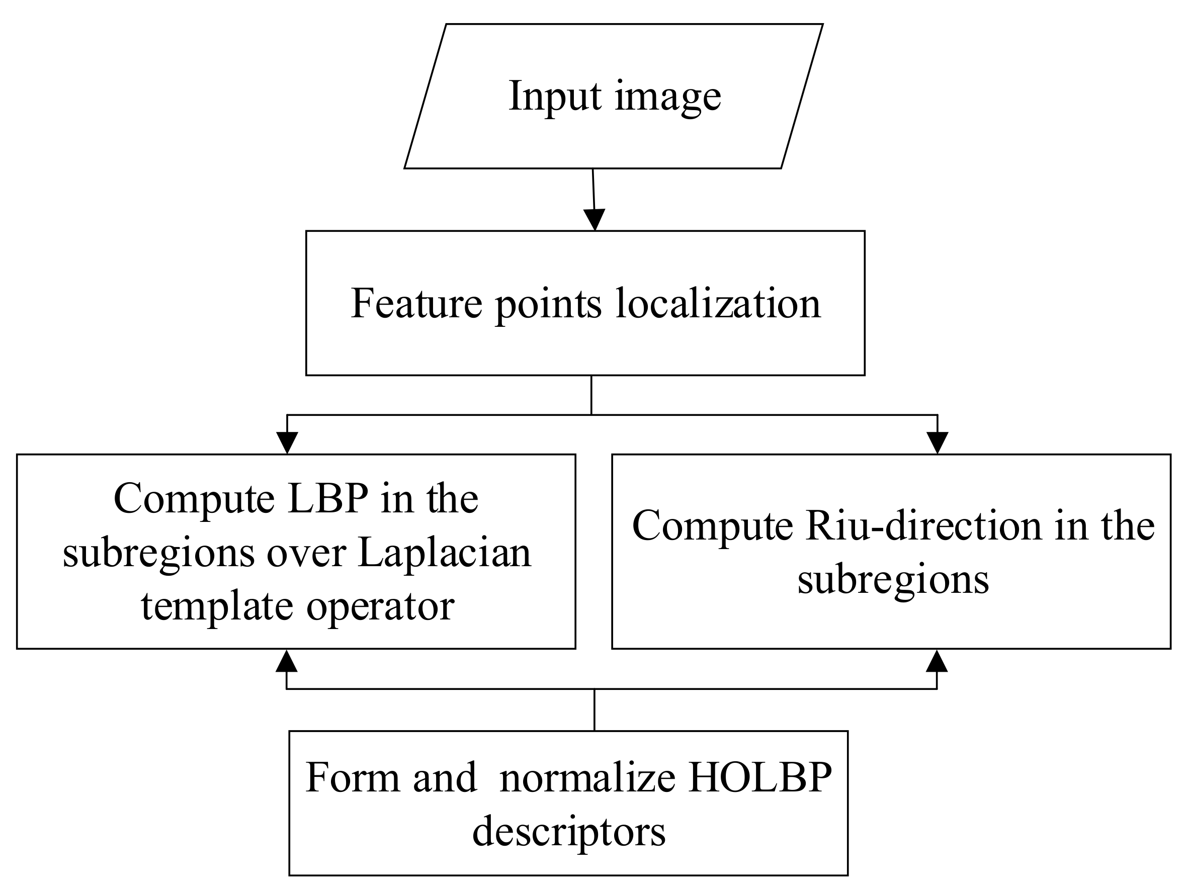
The 10-dimensional descriptor added in this step can include the direction change information around the feature points. It increases the abundance of the description information with 8 directions. Figure 3 summarizes the flowchart of HOLBP. Next, it is necessary to make a preliminary selection handling a large amount of descriptor information of an image.

2.4. Matching Assignment

For initial matching, we use the Euclidean squared distance as a measure of the similarity between the two image descriptors, and we compare the nearest distance obtained after sorting with the second nearest distance, if:
d n < d s n × d r a t i o
where d n indicates the nearest-neighbor distance, d s n indicates the second-nearest-neighbor distance, and d r a t i o ( 0 , 1 ) is the matching threshold. In this article, d r a t i o = 0.9 .
The feature points satisfying the above formula are initially matched. For most statistical problems, the Euclidean distance is unsatisfactory. Thus, we applied RANSAC [24] to select a set of inliers compatible with a homography between the images, and we verified the match using a probabilistic model.
For a pair of matching points in the picture, we have the following relationship:
p H q
which can be expanded to:
x p y p 1 H 11 H 12 H 13 H 21 H 22 H 23 H 31 H 32 1 x q y q 1
where p and q are a pair of matching points, the coordinates of which are respectively ( x p , y p ) and ( x q , y q ) , H represents a homography matrix, and denotes the proportional relationship.
Four random sample sets are selected, and the homography matrix H between them is calculated by LSM (least squares template matching). Following this, we handle the remaining point sets in the reference image and H to predict the coordinates of the image to be registered. After iterations, the largest inlier sets (whose projections are consistent with H) are found, and the H generated is the transformation matrix between two images.
Assume that the point sets obtained after preliminary matching are P = p 1 , p 2 , , p n and Q = q 1 , q 2 , , q n . For the first iteration, four sets of points are randomly selected from them, namely: P 1 = p 1 m , p 2 m , p 3 m , p 4 m and Q 1 = q 1 m , q 2 m , q 3 m , q 4 m , where the subscripts i m represent four randomly selected points, i = 1 , 2 , 3 , 4 . Note that they are not arranged in order, we record them in the above way for convenience.
In the previous section, we calculated the Riu gradient direction of the feature points. In the matching assignment, we exploited this information to improve the matching efficiency and filter randomly selected points in each iteration. θ max ( ) and θ min ( ) represent the maximum and minimum Riu directions, respectively, corresponding to the randomly selected sets. The randomly selected points should satisfy the following formula:
θ 1 max ( p i m ) θ 1 max ( q i m ) < ( θ 1 max ( p i m ) θ 1 max ( q i m ) ) ( θ 1 min ( p i m ) θ 1 min ( q i m ) )
where θ 1 ( ) indicates the Riu direction of the random point selected for the first iteration.
Then, we use the LSM algorithm and the coordinates of the points in P 1 to estimate the homography matrix H 1 . This process can be described by the following formula:
Q 1 ( x , y ) = H 1 P 1 ( x , y )
if,
q k ( x , y ) H t p k ( x , y ) 2 × max ( θ max ( p k ( x , y ) ) θ max ( q k ( x , y ) ) ) < T h r e s h o l d
where k = 1 , 2 , , n , and we output the number of points satisfying the above formula n k . We repeat the iterations until the maximum number of point sets n k max is reached, and we use the H k max obtained at this time as the final result.
We have the following iterative equation:
θ t max ( p i m ) θ t max ( q i m ) < ( θ t max ( p i m ) θ t max ( q i m ) ) ( θ t min ( p i m ) θ t min ( q i m ) ) Q t ( x , y ) = H t P t ( x , y ) d k = q k ( x , y ) H t p k ( x , y ) 2 × max ( θ max ( p k ( x , y ) ) θ max ( q k ( x , y ) ) ) d k < T h r e s h o l d , p k P max ( k ) , q k Q max ( k ) 0 < t < t max
where t is the number of iterations, θ t ( ) indicates the Riu direction of the random point selected for the tth iteration, P t = p 1 m , p 2 m , p 3 m , p 4 m , and Q t = q 1 m , q 2 m , q 3 m , q 4 m . p k ( x , y ) and q k ( x , y ) are both included in P ( x , y ) and Q ( x , y ) , respectively. In this paper, t max = 1000 , and we set T h r e s h o l d = 0 . 4 at each iteration. The steps of the proposed method are outlined in Algorithm 1.
Algorithm 1 Proposed Algorithm
Input: < P , Q >: The initial matching points through nearest-neighbor distance ratio. P = p 1 , p 2 , , p n , Q = q 1 , q 2 , , q n .
Output: < P max , Q max >: The final matching set updated by the proposed method.
Step1: Obtain sets < P t , Q t > by Equation (12).
                   If θ t max ( p i m ) θ t max ( q i m ) < ( θ t max ( p i m ) θ t max ( q i m ) ) ( θ t min ( p i m ) θ t min ( q i m ) )
                  P t = p 1 m , p 2 m , p 3 m , p 4 m , Q t = q 1 m , q 2 m , q 3 m , q 4 m
                   End If
Step2: Estimate the homography matrix H t by Equation (13).
                Q t ( x , y ) = H t P t ( x , y )
Step3: Obtain sets < P max ( k ) , Q max ( k ) > by Equation (14).
          For k = 1 : n
                  d k = q k ( x , y ) H t p k ( x , y ) 2 × max ( θ max ( p k ( x , y ) ) θ max ( q k ( x , y ) ) )
                 If d k < T h r e s h o l d
                  p k P max ( k ) , q k Q max ( k )
                 End If
          End For
Step4: Obtain sets < P max , Q max > by repeating the iterations.
          For t = 1 : t max , n 0 = 0 , n k = s i z e ( P max ( k ) )
                 If n k > n 0
                    n 0 n k + n 0 , P max P max ( k ) , Q max Q max ( k )
                 End If
              End For

3. Experimental Results and Analysis

In this section, the experimental data and results are analyzed in detail, including remote sensing image data, experimental evaluation measurements, and the displayed results. All the experiments were conducted with the MATLAB R2016b software on a computer with an Intel Core 3.2 GHz processor and 8.0 GB of physical memory.

3.1. Data

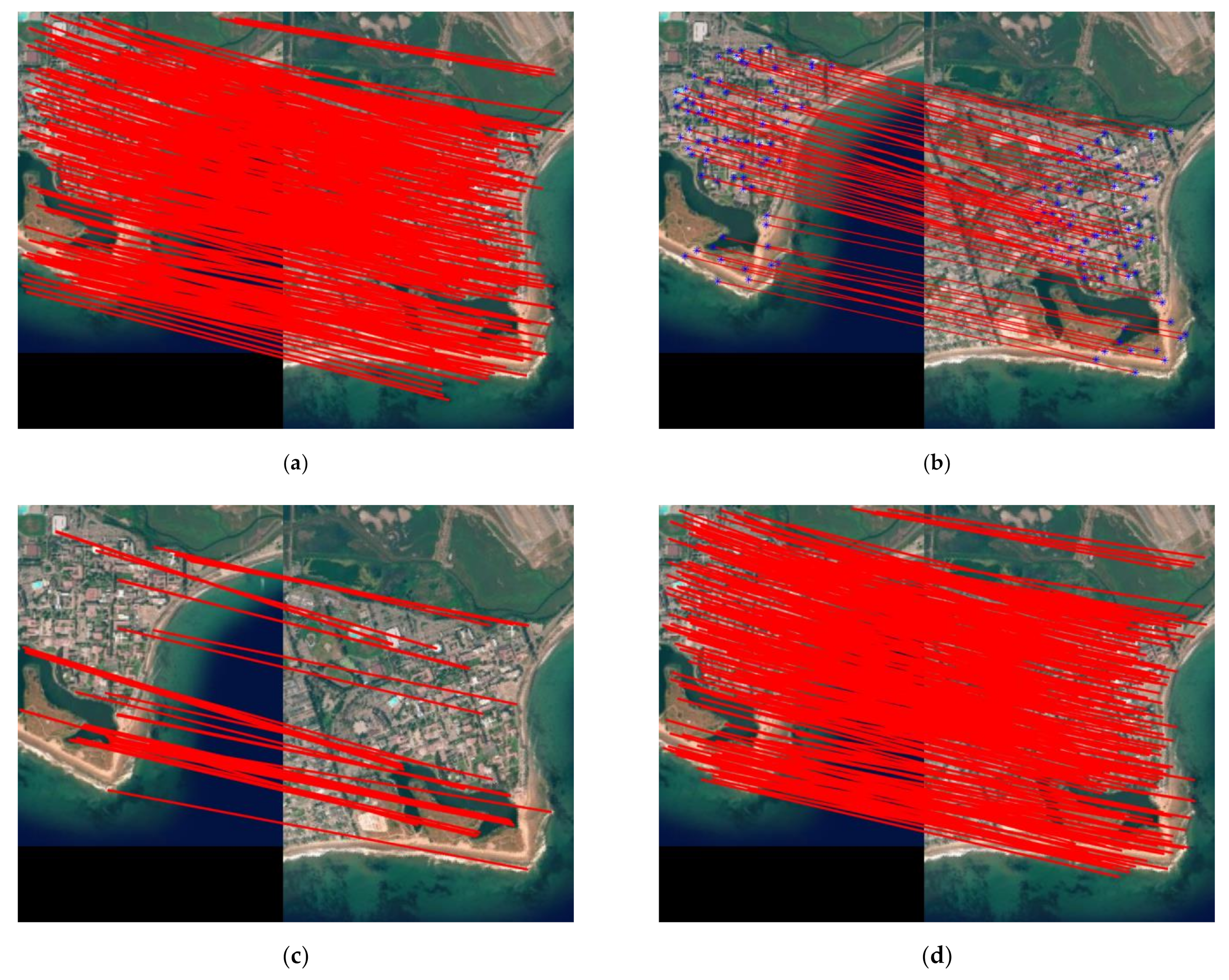
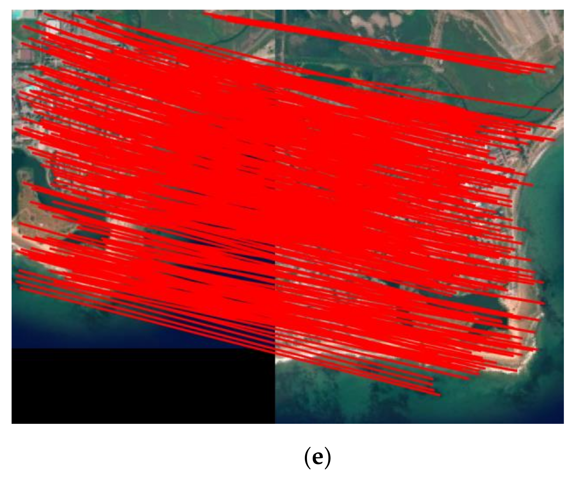
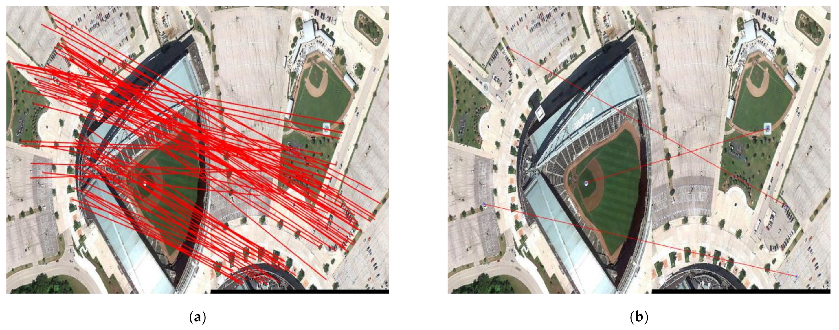
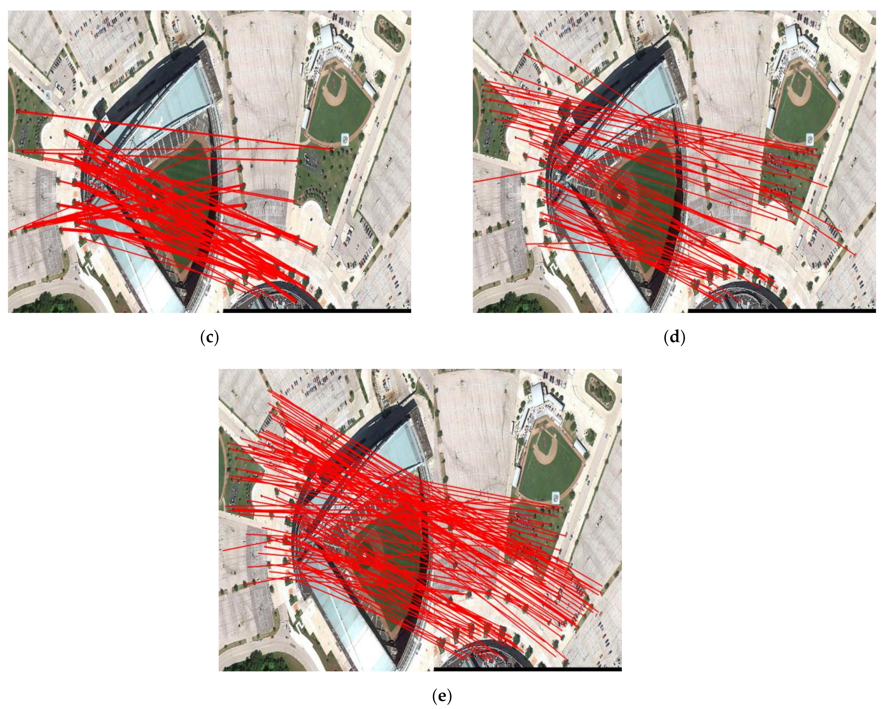
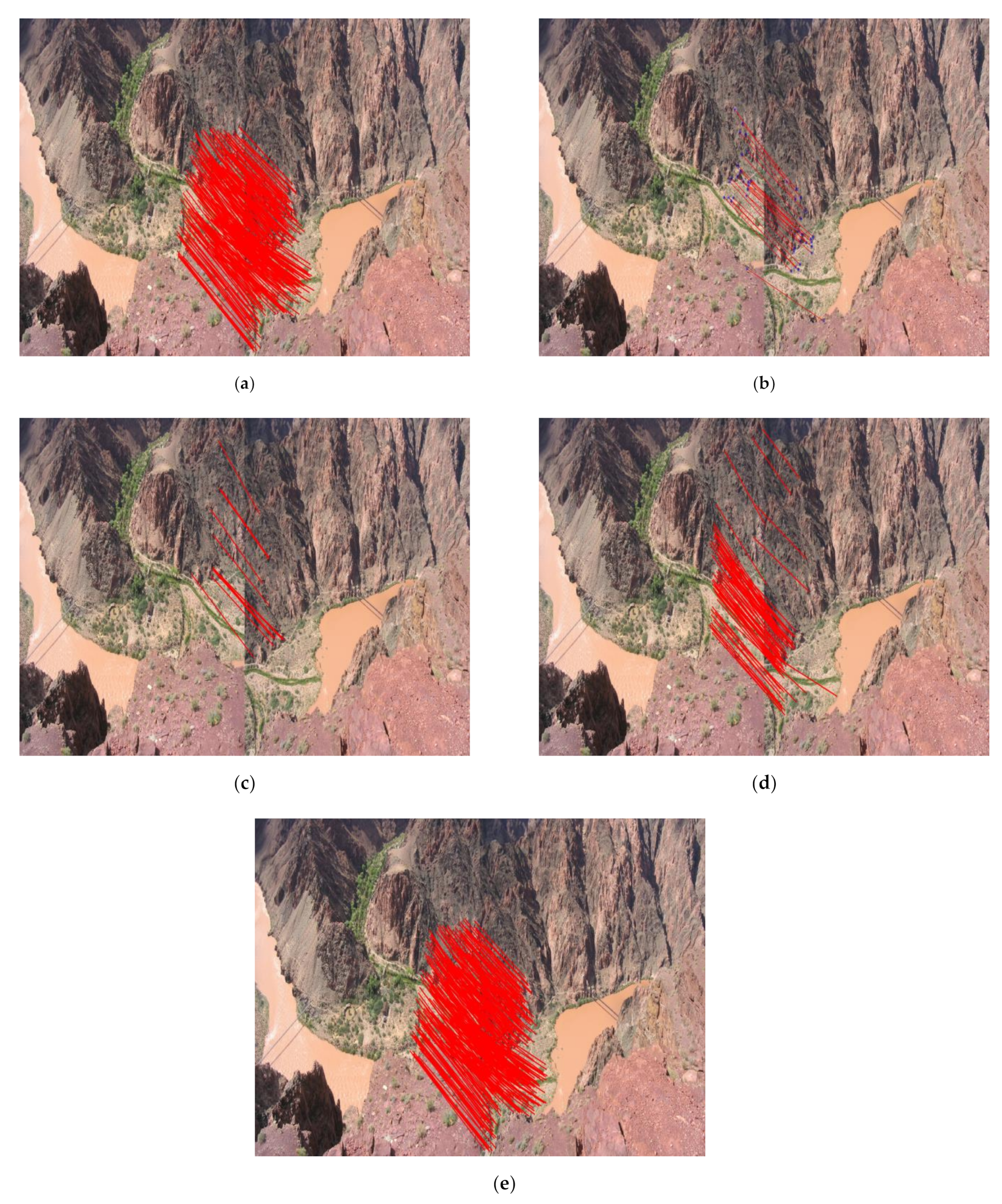
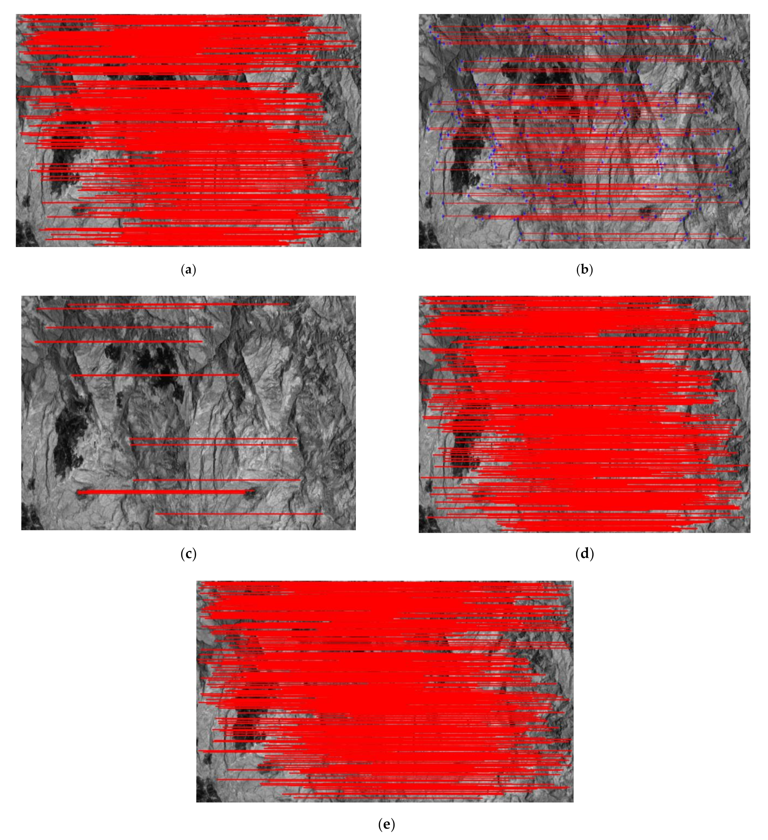
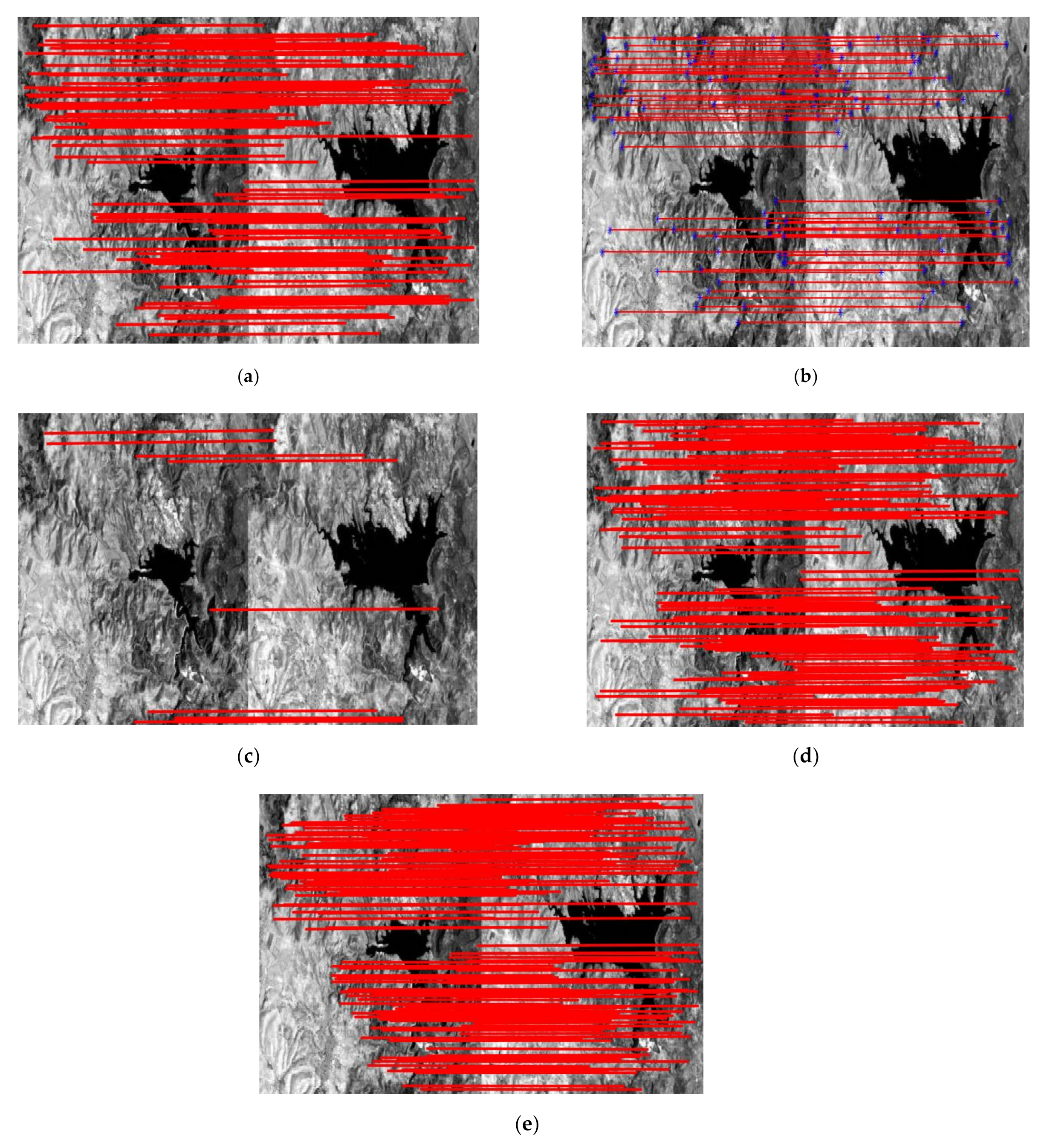
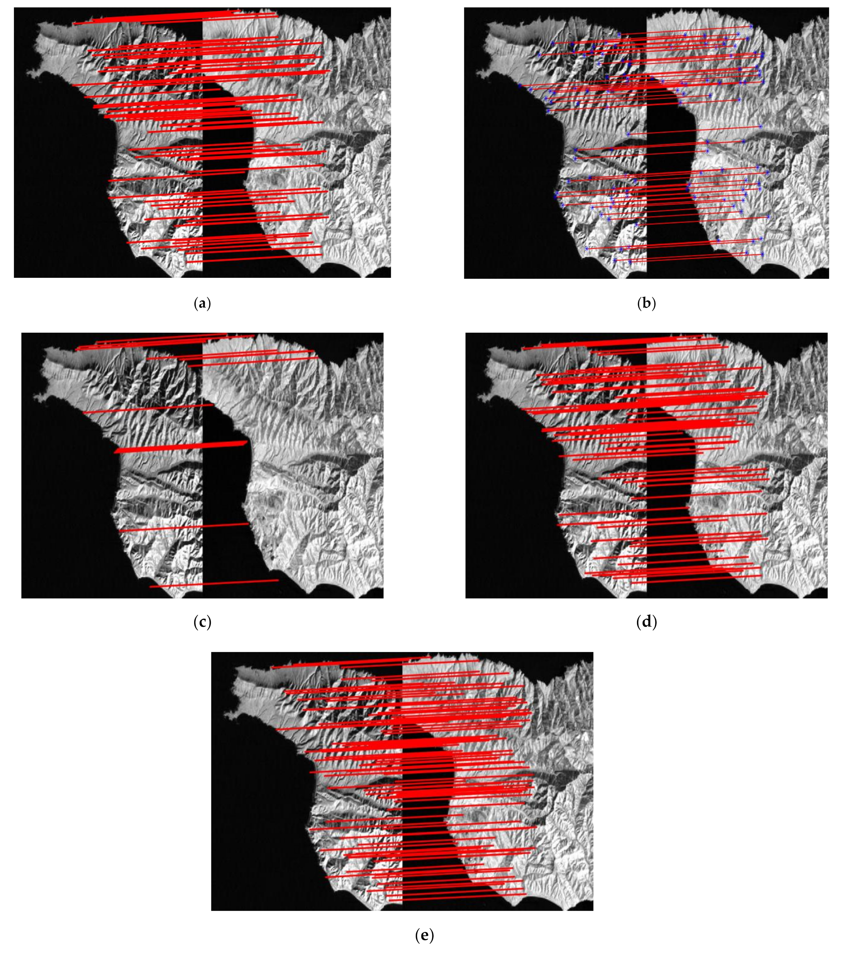
Six pairs of images were selected to test the performance of our method. Table 1 gives a detailed description of each pair, and Figure 4, Figure 5, Figure 6, Figure 7, Figure 8 and Figure 9 and Table 2, Table 3, Table 4, Table 5, Table 6 and Table 7 show the registration results of images for different methods. Table 8 summarizes the registration results of images for different methods. The bolded values of all the tables represent the method with best performance under different evaluations. The symbol of “*” means that registration failed (RMSE > 4).

3.2. Experimental Evaluations

3.2.1. Number of Correct Matches

The number of correct matching points can indicate the effectiveness of a method under the same conditions.

3.2.2. Registration Accuracy

The root mean-square error (RMSE) is used to measure the deviation between the observed value and the true value [11,21], which can be denoted as:
R M S E = 1 N i = 1 N ( ( x i x ˜ i ) 2 + ( y i y ˜ i ) 2 )
where ( x i , y i ) and ( x i , y i ) are those of the N selected key points from the image pair, and ( x ˜ i , y ˜ i ) denotes the transformed coordinates of ( x i , y i ) .
The RMSE is more sensitive to outliers. If there is a large difference between the predicted value and the true value, the RMSE will be very large.

3.2.3. Total Time

The less time that is spent, the better the method is in real-time.

3.3. Results Analysis

We compared the proposed method with SIFT+RANSAC [24], SURF [25], SAR-SIFT [26], and PSO-SIFT [21] to verify the effectiveness, accuracy, and feasibility. There were no deep learning (DL)-related methods used in the comparisons, as DL typically uses 80% or more of a dataset for training while we used 2% of a dataset for training or no training at all. The experimental results are shown in Table 8, where 307 and 73 represent the number of correct matching pairs, 0.3226 and 0.5850 represent the RMSEs, and 7.153 and 10.239 denote the computation time in seconds.
In the experimental test, we selected six remote sensing test images, which can be divided into large rotation angle and almost constant rotation angle. It can be observed from Table 8 that our method could achieve satisfactory results regardless of whether or not the registration images had very large rotation angles. The following is our specific analysis.
Table 8 shows that on the Pair-A, Pair-B, and Pair-C test images, i.e., when angle deviations of the test images change significantly, our method could extract as many correct matching points as possible while also achieving smaller RMSEs. Without the support of rotation-invariant angle information, the traditional SIFT could achieve a good registration effect, but it lost its competitiveness in comparison with our method. Both SURF and SAR-SIFT showed that the registration effect on these three pairs of test images was inadequate.
On the Pair-D, Pair-E, and Pair-F test images, i.e., the test images having almost constant rotation direction, Table 8 also shows the superiority of the HOLBP descriptors. In other words, considering the same image information, our novel descriptor could extract the texture and contour information of an image to the greatest extent, which is reflected in the correct matching points and RMSEs.
Although SIFT+RANSAC was almost on par with our method when images were not affected by angle changes, it lost its preponderance in terms of correct matching points, as shown in the results. It can be seen from Table 8 that our method could find more correct matching points with little RMSE loss. In particular, when the test image had strong texture information, such as Pair-D, Pair-E, and Pair-F, the differences between both approaches were more obvious. It is the HOLBP descriptor based on the construction of rotation-invariant texture information rather than the original SIFT descriptor that detects more pairs of matching points. Even though SURF has an advantage in terms of speed, its instability in RMSE and mismatches are unacceptable. Even though PSO-SIFT has better matching accuracy, the time loss cannot be ignored. In general, our method outperformed others, yet it also demonstrated some deficiency in sample matching precision.
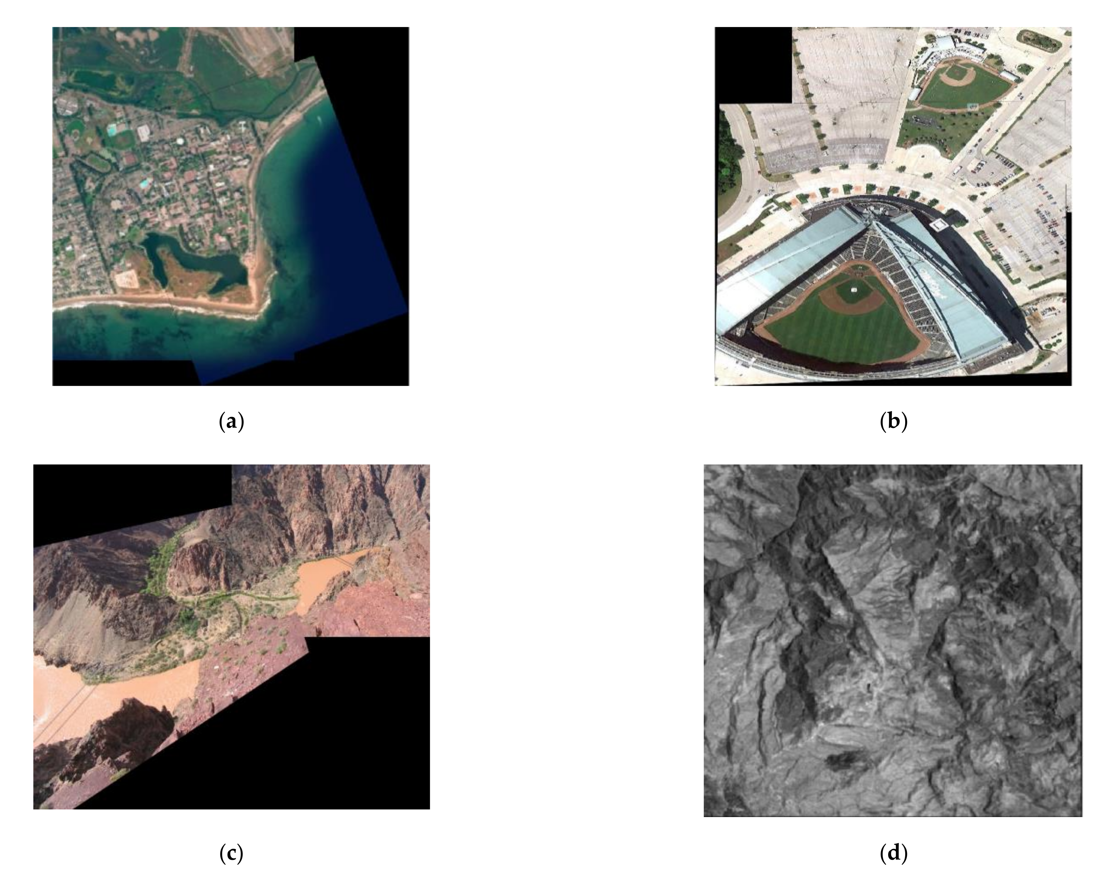
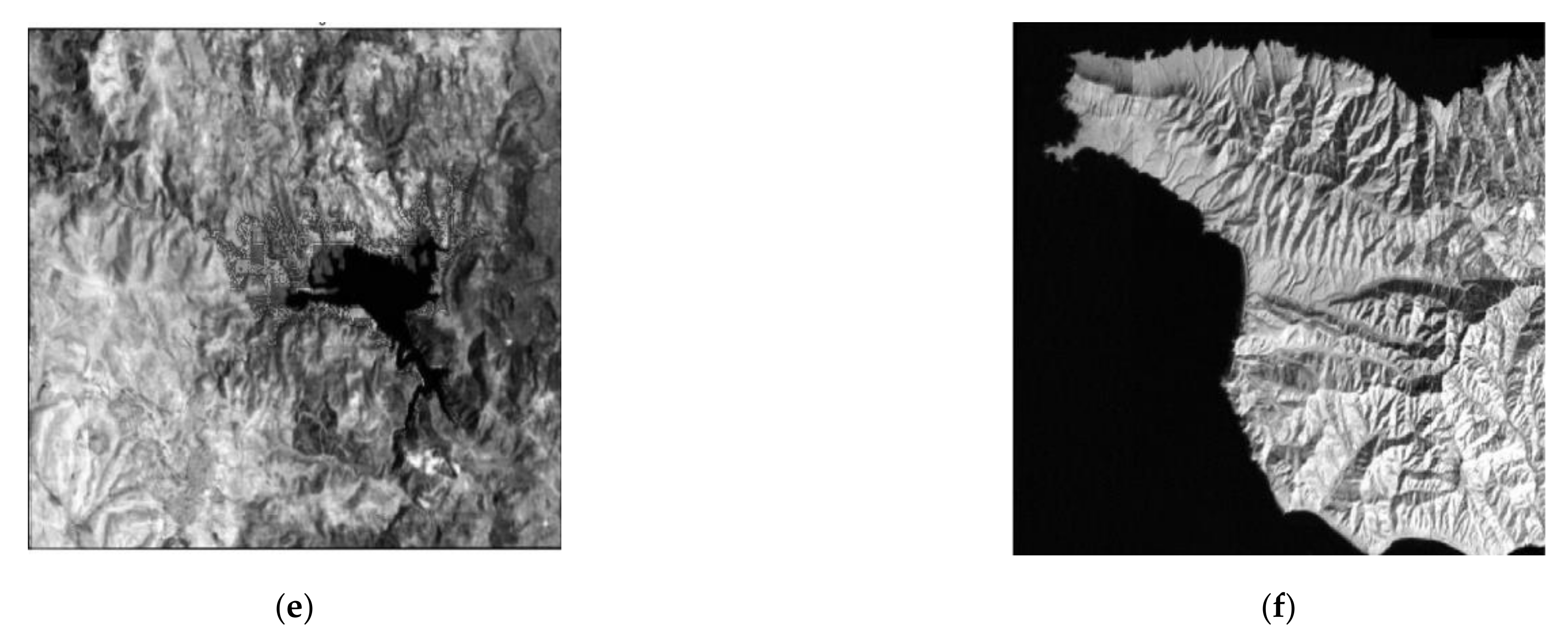
In order to further verify the accuracy and effectiveness, Figure 10 shows the registration results on six pairs of images. In general, comparing four methods and test images of different sizes and types, our method was very stable under the three experimental evaluations, and the registration results were also satisfactory.

4. Conclusions

We proposed a novel method to construct descriptors, called HOLBP, for fast and robust matching, and we redefined the gradient and direction calculation template. Experimental results demonstrated that our methods had advantages in terms of correct matching points, and registration accuracy and time, making our method stable on different test images and remote sensing image registration.
However, in the experiments, we found that the effect of real noise still could not be eliminated. Secondly, for some images with low resolution, we lost the dominant position. Our method aimed to obtain more of the correct matched points but yielded poor RMSE, for example, Table 5, Table 6 and Table 7, which was not satisfactory. In future work, we will focus on ameliorating the accuracy and improving the speed of matching for a larger variety of remote sensing images. We will also investigate the use of other transforms, like the Radon transform [27,28], for remote sensing image registration.

Author Contributions

Conceptualization, Y.H. and X.Z.; algorithm design, Y.H. and C.L.; experiments design, Y.H., C.L., A.B. and Z.P.; experiments conduction, Y.H. and X.Z.; data curation, C.L. and Z.P.; writing—original draft preparation, Y.H. and X.Z.; writing—review and editing, C.L., A.B. and I.C.; supervision, I.C.; funding acquisition, C.L., A.B. and I.C. All authors have read and agreed to the published version of the manuscript.

Funding

This work was supported in part by the National Natural Science Foundation of China under Grant 61702251, Grant 61971273, and Grant 11571011; in part by the Doctor Scientific Research Starting Foundation of Northwest University under Grant 338050050; in part by the Youth Academic Talent Support Program of Northwest University; in part by the Natural Science Foundation of Guangdong Province under Grant 2018A030310688; in part by the Young Innovative Talents Project in Ordinary University of Guangdong Province under Grant 601821K37052; and in part by NSERC Canada.

Institutional Review Board Statement

Not applicable.

Informed Consent Statement

Not applicable.

Data Availability Statement

Data will be available upon request to the corresponding author.

Conflicts of Interest

The authors declare no conflict of interest.

References

  1. Zitová, B.; Flusser, J. Image registration methods: A survey. Image Vis. Comput. 2003, 21, 977–1000. [Google Scholar] [CrossRef] [Green Version]
  2. Xiong, B.; Jiang, W.; Li, D.; Qi, M. Voxel Grid-Based Fast Registration of Terrestrial Point Cloud. Remote Sens. 2021, 13, 1905. [Google Scholar] [CrossRef]
  3. Ayhan, B.; Dao, M.; Kwan, C.; Chen, H.-M.; Bell, J.F.; Kidd, R. A Novel Utilization of Image Registration Techniques to Process Mastcam Images in Mars Rover with Applications to Image Fusion, Pixel Clustering, and Anomaly Detection. IEEE J. Sel. Top. Appl. Earth Obs. Remote Sens. 2017, 10, 4553–4564. [Google Scholar] [CrossRef]
  4. Lu, J.; Jia, H.; Li, T.; Li, Z.; Ma, J.; Zhu, R. An Instance Segmentation Based Framework for Large-Sized High-Resolution Remote Sensing Images Registration. Remote Sens. 2021, 13, 1657. [Google Scholar] [CrossRef]
  5. Wu, S.; Zhong, R.; Li, Q.; Qiao, K.; Zhu, Q. An Interband Registration Method for Hyperspectral Images Based on Adaptive Iterative Clustering. Remote Sens. 2021, 13, 1491. [Google Scholar] [CrossRef]
  6. Yu, N.; Wu, M.J.; Liu, J.X.; Zheng, C.H.; Xu, Y. Correntropy-based hypergraph regularized NMF for clustering and feature selection on multi-cancer integrated data. IEEE Trans. Cybern. 2020. [Google Scholar] [CrossRef] [PubMed]
  7. Cai, G.; Su, S.; Leng, C.; Wu, Y.; Lu, F. A Robust Transform Estimator Based on Residual Analysis and Its Application on UAV Aerial Images. Remote Sens. 2018, 10, 291. [Google Scholar] [CrossRef] [Green Version]
  8. Zhang, H.P.; Leng, C.C.; Yan, X.; Cai, G.R.; Pei, Z.; Yu, N.G.; Basu, A. Remote sensing image registration based on local affine constraint with circle descriptor. IEEE Geosci. Remote Sens. Lett. 2020. [Google Scholar] [CrossRef]
  9. Zhang, J.; Ma, W.P.; Wu, Y.; Jiao, L.C. Multimodal remote sensing image registration based on image transfer and local features. IEEE Geosci. Remote Sens. Lett. 2019, 16, 1210–1214. [Google Scholar] [CrossRef]
  10. Li, Q.L.; Wang, G.Y.; Liu, J.G.; Chen, S.B. Robust scale-invariant feature matching for remote sensing image registration. IEEE Geosci. Remote Sens. Lett. 2009, 6, 287–291. [Google Scholar]
  11. Ma, W.P.; Zhang, J.; Wu, Y.; Jiao, L.C.; Zhu, H.; Zhao, W. A novel two-step registration method for remote sensing images based on deep and local features. IEEE Trans. Geosci. Remote Sens. 2019, 57, 4834–4843. [Google Scholar] [CrossRef]
  12. Awrangjeb, M.; Lu, G.J. Techniques for efficient and effective transformed image identification. J. Vis. Commun. Image Represent. 2009, 20, 511–520. [Google Scholar] [CrossRef] [Green Version]
  13. Ye, Y.X.; Shan, J.; Bruzzone, L.; Shen, L. Robust registration of multimodal remote sensing image based on structural similarity. IEEE Trans. Geosci. Remote Sens. 2017, 55, 2941–2958. [Google Scholar] [CrossRef]
  14. Ye, Y.X.; Bruzzone, L.; Shan, J.; Bovolo, F.; Zhu, Q. Fast and robust matching for multimodal remote sensing image registration. IEEE Trans. Geosci. Remote Sens. 2019, 57, 9059–9070. [Google Scholar] [CrossRef] [Green Version]
  15. Wu, Y.; Ma, W.P.; Gong, M.G.; Su, L.Z.; Jiao, L.C. A novel point-matching algorithm based on fast sample consensus for image registration. IEEE Geosci. Remote Sens. Lett. 2015, 12, 43–47. [Google Scholar] [CrossRef]
  16. Ma, J.Y.; Zhao, J.; Tian, J.W.; Yuille, A.L.; Tu, Z.W. Robust point matching via vector field consensus. IEEE Trans. Image Process. 2014, 23, 1706–1721. [Google Scholar] [CrossRef] [Green Version]
  17. Ma, J.Y.; Zhao, J.; Jiang, J.J.; Zhou, H.B.; Guo, X.J. Locality preserving matching. Int. J. Comput. Vis. 2019, 127, 512–531. [Google Scholar] [CrossRef]
  18. Ma, J.Y.; Jiang, J.J.; Zhou, H.B.; Zhao, J.; Guo, X.J. Guided locality preserving feature matching for remote sensing image registration. IEEE Trans. Geosci. Remote Sens. 2018, 56, 4435–4447. [Google Scholar] [CrossRef]
  19. Jiang, X.Y.; Jiang, J.J.; Fan, A.X.; Wang, Z.Y.; Ma, J.Y. Multiscale locality and rank preservation for robust feature matching of remote sensing images. IEEE Trans. Geosci. Remote Sens. 2019, 57, 6462–6472. [Google Scholar] [CrossRef]
  20. Lowe, D.G. Distinctive image features from scale-invariant keypoints. Int. J. Comput. Vis. 2004, 60, 91–110. [Google Scholar] [CrossRef]
  21. Ma, W.P.; Wen, Z.L.; Wu, Y.; Jiao, L.C.; Gong, M.G.; Zheng, Y.F.; Liu, L. Remote sensing image registration with modified SIFT and enhanced feature matching. IEEE Geosci. Remote Sens. Lett. 2017, 14, 3–7. [Google Scholar] [CrossRef]
  22. Chang, H.H.; Wu, G.L.; Chiang, M.H. Remote sensing image registration based on modified SIFT and feature slope grouping. IEEE Geosci. Remote Sens. Lett. 2019, 16, 1363–1367. [Google Scholar] [CrossRef]
  23. Ojala, T.; Pietikainen, M.; Maenpaa, T. Multiresolution gray-scale and rotation invariant texture classification with local binary patterns. IEEE Trans. Pattern Anal. Mach. Intell. 2002, 24, 971–987. [Google Scholar] [CrossRef]
  24. Hong, W.W.J.; Tang, Y.P. Image matching for geomorphic measurement based on SIFT and RANSAC methods. In Proceedings of the 2008 International Conference on Computer Science and Software Engineering, Wuhan, China, 12–14 December 2008; Volume 2, pp. 317–320. [Google Scholar]
  25. Bay, H.; Ess, A.; Tuytelaars, T.; Gool, L.V. Speeded-up robust features. Comput. Vis. Image Underst. 2008, 110, 404–417. [Google Scholar] [CrossRef]
  26. Dellinger, F.; Delon, J.; Gousseau, Y.; Michel, J.; Tupin, F. SAR-SIFT: A SIFT-like algorithm for SAR images. IEEE Trans. Geosci. Remote Sens. 2015, 53, 453–466. [Google Scholar] [CrossRef] [Green Version]
  27. Singh, M.; Mandal, M.; Basu, A. Visual gesture recognition for ground air traffic control using the Radon transform. In Proceedings of the IEEE/RSJ International Conference on Intelligent Robots and Systems, Edmonton, AB, Canada, 2–6 August 2005; pp. 2586–2591. [Google Scholar]
  28. Singh, M.; Mandal, M.; Basu, A. Pose recognition using the Radon transform. In Proceedings of the IEEE Midwest Symposium on Circuits and Systems, Covington, KY, USA, 7–10 August 2005; pp. 1091–1094. [Google Scholar]
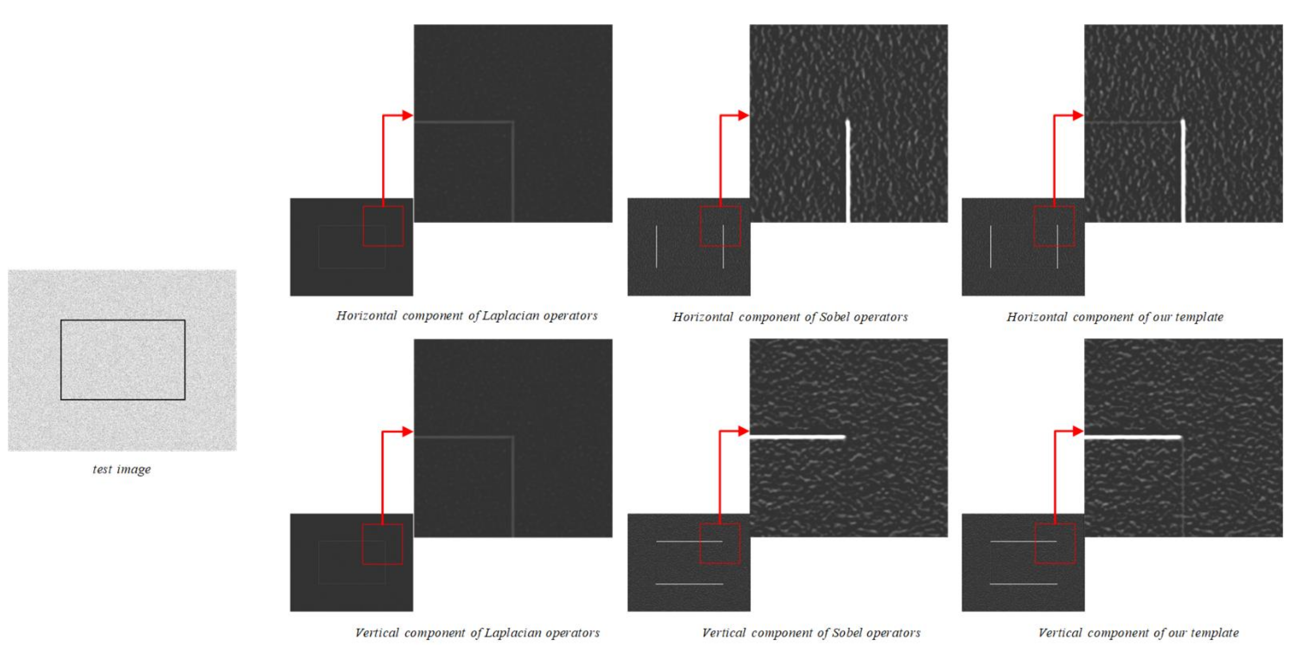
Figure 1. Three different gradient computations applied on the test image.
Remotesensing 13 02328 g001
Figure 2. (a) Subregion of HOLBP descriptor. (b) The circular neighborhood of eight sample points.
Remotesensing 13 02328 g002
Figure 3. Flowchart of HOLBP.
Remotesensing 13 02328 g003
Figure 4. Matching results of different methods for images of Pair-A: (a) SIFT+RANSAC; (b) SURF; (c) SAR-SIFT; (d) PSO-SIFT; (e) our method.
Remotesensing 13 02328 g004aRemotesensing 13 02328 g004b
Figure 5. Matching results of different methods for images of Pair-B: (a) SIFT+RANSAC; (b) SURF; (c) SAR-SIFT; (d) PSO-SIFT; (e) our method.
Remotesensing 13 02328 g005aRemotesensing 13 02328 g005b
Figure 6. Matching results of different methods for images of Pair-C: (a) SIFT+RANSAC; (b) SURF; (c) SAR-SIFT; (d) PSO- SIFT; (e) our method.
Remotesensing 13 02328 g006
Figure 7. Matching results of different methods for images of Pair-D: (a) SIFT+RANSAC; (b) SURF; (c) SAR-SIFT; (d) PSO-SIFT; (e) our method.
Remotesensing 13 02328 g007
Figure 8. Matching results of different methods for images of Pair-E: (a) SIFT+RANSAC; (b) SURF; (c) SAR-SIFT; (d) PSO-SIFT; (e) our method.
Remotesensing 13 02328 g008
Figure 9. Matching results of different methods for images of Pair-F: (a) SIFT+RANSAC; (b) SURF; (c) SAR-SIFT; (d) PSO-SIFT; (e) our method.
Remotesensing 13 02328 g009
Figure 10. Registration results of our method: (a) Pair-A after registration; (b) Pair-B after registration; (c) Pair-C after registration; (d) Pair-D after registration; (e) Pair-E after registration; (f) Pair-F after registration.
Remotesensing 13 02328 g010aRemotesensing 13 02328 g010b
Table 1. Detailed description of six pair images.
PairSensor and DataSizeImage Characteristic
Pair-ARemote sensing image data set306 × 386Geographic images
Remote sensing image data set472 × 355
Pair-BADS 40, SH52/August 6, 2008 811   × 705Stadium in Stuttgart, Germany
ADS 40, SH52/August 6, 2008 709   × 695
Pair-CRemote sensing image data set 768   × 1024mountain chain
Remote sensing image data set 768   × 1024
Pair-DLandsat-7/ April, 2000 512   × 512Mexico
Landsat-7/May, 2002 512   × 512
Pair-ELandsat-5/September, 1995 412   × 300Sardinia
Landsat-5/July, 1996 312   × 300
Pair-FRemote sensing image data set 400   × 400Geographic images
Remote sensing image data set 400   × 400
Table 2. The number of matches and key points, running time, and comparisons of RMSE of different methods for Pair-A.
MethodsSIFT+RANSACSURFSAR-SIFTPSO-SIFTOur Method
Number of Matches/Key points307/35070/9941/96298/561325/360
Time/s7.1536.4066.2559.02610.181
RMSE0.32260.50570.66450.32170.3980
Table 3. The number of matches and key points, running time, and comparisons of RMSE of different methods for Pair-B.
MethodsSIFT+RANSACSURFSAR-SIFTPSO-SIFTOur Method
Number of Matches/Key points73/6163/212102/39254/455110/393
Time/s10.23910.5918.47818.82517.456
RMSE0.5850*0.59970.65500.7608
Table 4. The number of matches and key points, running time, and comparisons of RMSE of different methods for Pair-C.
MethodsSIFT+RANSACSURFSAR-SIFTPSO-SIFTOur Method
Number of Matches/Key points283/91722/28014/13277/883329/762
Time/s32.70112.05822.894169.66251.385
RMSE0.50240.55340.64400.61070.6143
Table 5. The number of matches and key points, running time, and comparisons of RMSE of different methods for Pair-D.
MethodsSIFT+RANSACSURFSAR-SIFTPSO-SIFTOur Method
Number of Matches/Key points449/971122/23718/117542/1196603/975
Time/s14.1518.4319.55650.27128.158
RMSE0.59880.59090.53810.61210.7449
Table 6. The number of matches and key points, running time, and comparisons of RMSE of different methods for Pair-E.
MethodsSIFT+RANSACSURFSAR-SIFTPSO-SIFTOur Method
Number of Matches/Key points111/33665/19811/103112/345166/325
Time/s6.7558.657.09112.32313.089
RMSE0.61680.55350.52930.64440.8219
Table 7. The number of matches and key points, running time, and comparisons of RMSE of different methods for Pair-F.
MethodsSIFT+RANSACSURFSAR-SIFTPSO-SIFTOur Method
Number of Matches/Key points83/29259/18116/14178/37297/244
Time/s6.6249.508.27710.83311.661
RMSE0.57340.56020.46910.63880.7570
Table 8. Correct matching numbers, comparisons of RMSE, and running time of different methods.
MethodsPair-APair-BPair-CPair-DPair-EPair-F
SIFT+RANSAC307/0.3226 /7.15373/0.5850/10.239283/0.5024/32.701449/0.5988/14.151111/0.6168/6.75583/0.5734/6.624
SURF70 /0.5057/6.4063/*/10.5922/0.5534/12.058122/0.5909/8.43165/0.5535/8.6559/0.5602/9.50
SAR-SIFT41/0.6645/6.255102/0.5997/18.47814/0.6440/22.89418/0.5381/9.55611/0.5293/7.09116/0.4691/8.277
PSO-SIFT298/0.3217/9.02654/0.6550/18.82577/0.5107/169.662542/ 0.6121/50.271112/0.6444/12.32378/0.6388/10.833
Our method325/0.3980/10.181110/0.7608/17.456329/0.6143/51.385627/0.7463/26.51176/0.8796/13.74197/0.7570/11.661
Publisher’s Note: MDPI stays neutral with regard to jurisdictional claims in published maps and institutional affiliations.