Abstract
A deep-learning architecture, dubbed as the 2D-ADMM-Net (2D-ADN), is proposed in this article. It provides effective high-resolution 2D inverse synthetic aperture radar (ISAR) imaging under scenarios of low SNRs and incomplete data, by combining model-based sparse reconstruction and data-driven deep learning. Firstly, mapping from ISAR images to their corresponding echoes in the wavenumber domain is derived. Then, a 2D alternating direction method of multipliers (ADMM) is unrolled and generalized to a deep network, where all adjustable parameters in the reconstruction layers, nonlinear transform layers, and multiplier update layers are learned by an end-to-end training through back-propagation. Since the optimal parameters of each layer are learned separately, 2D-ADN exhibits more representation flexibility and preferable reconstruction performance than model-driven methods. Simultaneously, it is able to better facilitate ISAR imaging with limited training samples than data-driven methods owing to its simple structure and small number of adjustable parameters. Additionally, benefiting from the good performance of 2D-ADN, a random phase error estimation method is proposed, through which well-focused imaging can be acquired. It is demonstrated by experiments that although trained by only a few simulated images, the 2D-ADN shows good adaptability to measured data and favorable imaging results with a clear background can be obtained in a short time.
1. Introduction
High-resolution inverse synthetic aperture radar (ISAR) imaging plays a significant role in space situation awareness and air target surveillance [1,2]. Under ideal observational environments with high signal-to-noise ratios (SNRs) and complete echo matrices, well-focused imaging can be acquired by classic techniques such as the range-Doppler (RD) algorithm and the polar formatting algorithm (PFA) [3]. For a target with a small radar cross section (RCS) or a long observation distance, however, the SNR of the received echoes is low due to limited transmitted power. In addition, the existence of strong jamming and the resource scheduling of the cognitive radar may result in incomplete data along the range or/and azimuth direction(s). The complex observational environments discussed above, i.e., incomplete data and low SNRs, cause severe performance degradation or even invalidate the available imaging techniques. As ISAR images are generally sparse in the image domain, high-resolution ISAR imaging under complex observational environments based on the theory of sparse signal reconstruction has received intensive attention in the radar imaging community in recent years [4,5], in which the reconstruction of sparse images (i.e., the distribution of dominant scattering centers) from noisy or gapped echoes given the observation dictionary is sought.
In addition, the motion of the target can be decomposed into translational motion and rotational motion, where the former is not beneficial to imaging and needs to be compensated by range alignment and autofocusing. Traditional autofocusing algorithms can obtain satisfying imaging results from complete radar echoes [6]. For complex observational environments, however, they cannot achieve good performance due to the deficiency of radar echoes and low SNRs. In recent years, parametric autofocusing techniques [7] have been applied for sparse imaging. Although they are superior to traditional methods under sparse aperture conditions, their performance is dependent on imaging quality. Therefore, in turn, a better sparse reconstruction method is needed.
The available sparse ISAR imaging methods can be divided into three categories: (1) model-driven methods; (2) data-driven methods; and (3) combined model-driven and data-driven methods. Among them, model-driven methods construct the sparse observation model and obtain high-resolution images by -norm or -norm optimization. The -norm optimization, e.g., orthogonal MP (OMP) [8] and smoothed -norm method [9], cannot guarantee that the solution is sparsest and may converge to the local minima. The -norm optimization, e.g., the fast iterative shrinkage-thresholding algorithm (FISTA) [10,11] and alternating direction method of multipliers (ADMM) [12,13], is the convex approximation of the -norm [14]. However, the regularization parameter directly affects the performance and how to determine its optimum value remains an open problem [4]. Additionally, vectorized optimization requires long operating times and a large memory storage space. To improve the efficiency, methods based on matrix operations such as 2D-FISTA [15] and 2D-ADMM [16] are proposed.
Data-driven methods solve the nonlinear mapping from echoes to the 2D image by designing and training a deep network [17]. In the training process, the target echoes and corresponding ISAR images are adopted as the inputs and the label, respectively, and the loss function is the NMSE between the network output and the label. In order to minimize the loss function (i.e., to obtain the optimal network parameters), the network parameters are randomly initialized and updated by the gradient descent method iteratively until convergence [18]. Then, the trained network is applied to generate focused imaging of an unknown target. Facilitated by off-line network training, such methods achieve the reconstruction of multiple images rapidly, and typical networks include the complex-value deep neural network (CV-DNN) [19]. Nevertheless, the subjective network design process lacks unified criterion and theoretical support, which makes it difficult to analyze the influence of network structure and parameter settings on reconstruction performance. In addition, the large number of unknown parameters require massive training samples to avoid overfitting.
The combined model-driven and data-driven methods first expand the model-driven methods into a deep network [20], and then utilize only a few training samples to learn the optimal values of the adjustable parameters [21]. Finally, they output the focused image of an unknown target by the trained network. Such methods effectively solve the difficulties in: (1) setting proper parameters for model-driven methods; (2) clearly explaining the physical meaning of the network; and (3) generating a large number of training samples to avoid overfitting for data-driven methods. A common technique to expand the model-driven methods is unrolling [22], which utilizes a finite-layer hierarchical architecture to implement iterations. As a typical imaging network, the deep ADMM network [23] uses measured data for effective training, which is usually limited due to observation conditions, and autofocusing is not considered for sparse aperture ISAR imaging.
To tackle the above-mentioned problems, this article proposes the 2D-ADMM-Net (2D-ADN) to achieve well-focused 2D imaging under complex observational environments, and its key contributions mainly include the following: (a) Mapping from the ISAR images to echoes in the wavenumber domain is established, which forms as a 2D sparse reconstruction problem. Then, the 2D-ADMM method is provided with phase error estimation for focused imaging. (b) Based on the 2D-ADMM, 2D-ADN is designed to include the reconstruction layers, nonlinear transform layers, and multiplier update layers. Then, the adjustable parameters are estimated by minimizing the loss function through back-propagation in the complex domain. (c) Simulation results demonstrate that the 2D-ADN, which is trained by a small number of samples generated from point-scattering model, obtains the best reconstruction performance. For both the complete and incomplete data with low SNRs, the 2D-ADN combined with random phase error estimation obtains better-focused imaging of measured aircraft data with a clearer background than the available methods.
The remainder of this article is organized as follows. Section 2 establishes the sparse observation model for the high-resolution 2D imaging and provides the iterative formulae of 2D-ADMM with random phase error estimation. Section 3 introduces the construction of 2D-ADN in detail. Section 4 gives the network loss function and derives the back-propagation formulae in the complex domain. Section 5 carries out various experiments to prove the effectiveness of 2D-ADN. In Section 6, we discuss the performance of 2D-ADN, and Section 7 concludes the article with suggestions for future work.
2. Modeling and Solving
2.1. 2D Modeling
After translational motion compensation [24,25], echoes in the wavenumber domain satisfy:
where is the over-complete range dictionary, is the 2D distribution of the scattering centers, is the over-complete Doppler dictionary, is the complex noise matrix, and is the diagonal random phase error matrix.
In (2), denotes phase error of the th echo.
For convenience, we vectorized (1) as:
where is the vector form of , is the Kronecker product, , is the vector form of , and is the vector form of .
2.2. The 2D-ADMM Method
Finding the optimal solution to (3) is a linear inverse problem, which can be further converted into an unconstrained optimization by introducing the regularization term:
where is the regularization parameter.
According to the variable splitting technique [26], (4) is equivalent to:
and the augmented Lagrangian function is:
where is the inner product, is the vector of Lagrangian multiplier, and is the penalty parameter.
ADMM decomposes (6) into three sub-problems by minimizing with respect to , , and , respectively,
where is the iteration index. Let , the solutions to (7) satisfy:
where is the shrinkage function [27] defined by , is the threshold, and is an update rate for the Lagrangian multiplier.
The 2D-ADMM estimates the 2D image by:
In addition, the matrix forms of and , i.e., and , are calculated by,
2.3. Phase Error Estimation and Algorithm Summation
The phase error is estimated by optimizing the following objective function [28]:
where is the th column of , and is the th column of .
Let the derivative of (12) with respect to be zero, then:
where and represent the real and the imaginary parts, respectively, and the phase error matrix is constructed by (2).
Algorithm 1 summarizes the high-resolution 2D ISAR imaging and autofocusing method based on 2D-ADMM and random phase error estimation, where denotes the total number of iterations. Analysis and experiments have shown that the choice of and has a great influence on the imaging quality, and improper initialization may generate a defocused image with a noisy background. In addition, and cannot be adaptively adjusted in each iteration, demonstrating a lack of flexibility.
| Algorithm 1. Autofocusing by 2D-ADMM |
| 1. Initialize , , and |
| 2. For |
| For |
| Update by (9); |
| Update by (10); |
| Update by (11); |
| End |
| Calculate by (13) and (2); |
| End |
| 3. Output and |
3. Structure of 2D-ADN
To tackle the aforementioned problems, we modified 2D-ADMM and expanded it into 2D-ADN. There are similarities between deep networks and iterative algorithms [22] such as 2D-ADMM. Particularly, the matrix multiplication is similar to the linear mapping of the deep network, the shrinkage function is similar to the nonlinear operation, and the adjustable parameters are similar to network parameters. Therefore, the 2D-ADMM algorithm can be unfolded into 2D-ADN. As shown in Figure 1, the network has stages, and stage , , represents the th iteration described by Algorithm 1. Typically, one stage consists of three layers, i.e., the reconstruction layer, the nonlinear transform layer, and the multiplier update layer, which correspond to (9), (10), and (11), respectively. The inputs of 2D-ADN are echoes in the 2D wavenumber domain, and the output is the reconstructed 2D high-resolution image. Below, we will derive the forward-propagation formulae of each layer.
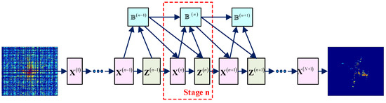
Figure 1.
Structure of the 2D-ADN.
3.1. Reconstruction Layer
As shown in Figure 2, the inputs of the reconstruction layer are and , and the output is:
where the penalty parameter is the adjustable parameter.
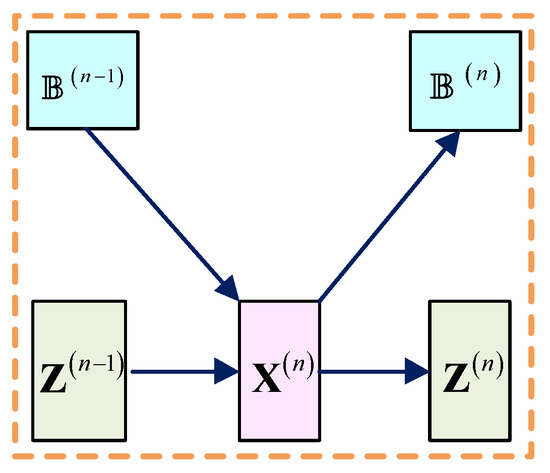
Figure 2.
Reconstruction layer.
For , and are initialized to zero matrices and thus the output is:
For , the output serves as the input of and . For , the output is adopted as the input of the loss function.
3.2. Nonlinear Transform Layer
As shown in Figure 3, the inputs of the nonlinear transform layer are and , and the output is:
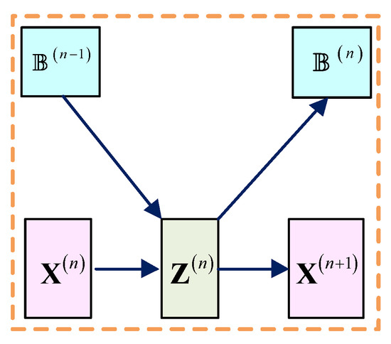
Figure 3.
Nonlinear transform layer.
To learn a more flexible non-linear activation function, we substituted a piecewise linear function for the shrinkage function [29]. Specifically, is determined by control points , where and denote the predefined position and adjustable value of the th point, respectively. In particular, we performed the on the real and imaginary parts of the complex signal, respectively.
For , is initialized as a zero matrix and the output is:
The output of this layer serves as the input of and .
3.3. Multiplier Update Layer
As shown in Figure 4, the inputs of the multiplier update layer are , , and , and the output is:
where the learning rate is an adjustable parameter.
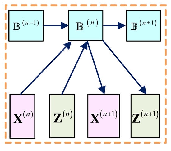
Figure 4.
Multiplier update layer.
For , is initialized as a zero matrix and the output is:
For , the output of this layer serves as the input of , , and . For , the output is adopted as the input of the reconstruction layer.
4. Training of 2D-ADN
4.1. Loss Function
In this article, the loss function is defined as the normalized mean square error (NMSE) between the network output and the label image , i.e., the ground truth of the scattering center distribution:
where are the input echoes in the wavenumber domain defined by (14), is the set of the adjustable parameters, is the Frobenius norm, and is the training set with .
4.2. Back-Propagation
We optimized the parameters of 2D-ADN utilizing the gradient-based limited-memory Broyden–Fletcher–Goldfarb–Shanno (L-BFGS) algorithm. To this end, we computed the gradients of the loss function with respect to through back-propagation over the deep architectures. Following the structures and writing styles of the available literatures dealing with deep networks [30] and the conjugate complex derivative of composite function [31], we derived the back-propagation of the three layers, respectively. To be consistent with the previous definition, the gradients of the matrices were expressed in matrix forms for convenience, and they were also calculated in matrix forms for efficiency.
As shown in Figure 5, the gradient transferred to the reconstruction layer through and for satisfies:
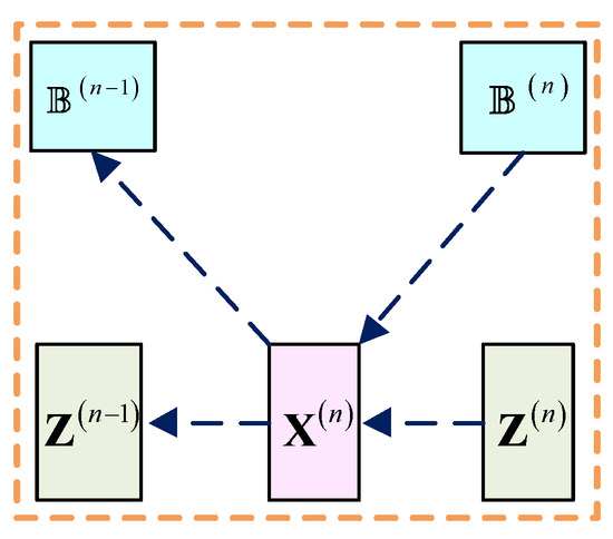
Figure 5.
Back-propagation of the reconstruction layer.
For , the gradient of the loss function transferred to equals to:
The gradient of is:
where:
and the gradients transferred to and are calculated by:
where:
where represents the matrix with all ones:
where:
As shown in Figure 6, the gradient transferred to the nonlinear transform layer through and satisfies:
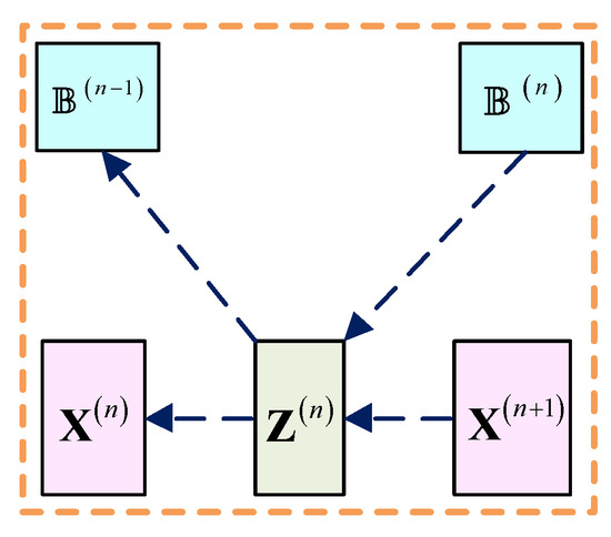
Figure 6.
Back-propagation of the nonlinear transform layer.
The gradient calculations of , , and are consistent with the derivation of the piecewise linear function defined in [29].
As shown in Figure 7, the gradient transferred to the multiplier update layer through , , and for satisfies:
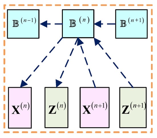
Figure 7.
Back-propagation of the multiplier update layer.
For , the gradient transferred from the last reconstruction layer to is:
The gradient of is:
where:
and the gradient of this layer transferred to , and are calculated by:
where:
where:
where:
The training stage can be summarized as follows:
Step1: Define the NMSE between the network output and the label image as the loss function;
Step2: Back-propagation. Calculate the gradients of the loss function with respect to the penalty parameter, the piecewise linear function, and the learning rate of each stage;
Step3: Utilize the L-BFGS algorithm to update the network parameters according to their current values and the gradients;
Step4: Repeat Step2~Step4 until the difference between the loss functions of the two adjacent iterations is less than 10−6.
For multiple training samples, we utilized the average gradient and loss function.
4.3. 2D High-Resolution ISAR Imaging Based on 2D-ADN
According to the above discussions, high-resolution 2D ISAR imaging based on 2D-ADN includes the following steps:
Step1: Training set generation. Initialize the phase error matrix , construct and according to the radar parameters and data missing pattern, generate randomly distributed scattering centers with Gaussian amplitudes, calculate according to (1), and obtain the data set .
Step2: Network training. Initialize the adjustable parameters , and utilize to train the network according to Section IV-B.
Step3: Testing. For simulated data, feed echoes in the wavenumber domain into the trained 2D-ADN and obtain the high-resolution image. For measured data with random phase errors, estimate the high-resolution image and random phase errors by the trained 2D-ADN and (13) iteratively until convergence.
As the distribution and the amplitudes of simulated scattering centers mimic true ISAR targets, optimal network parameters suitable for measured data imaging can be learned after network training. By this means, the issue of insufficient measured training data is effectively tackled.
In 2D-ADN the number of stages determines the network depth. It is observed that the loss function first decreases rapidly and then tends to be stable with the increment of . Therefore, we choose according to the convergence condition given below:
where is the loss function of the trained network with stages, is the loss function of the trained network with stages, and is a threshold.
For a single iteration, 2D-ADN and 2D-FISTA share the same computational complexity of . As the number of stages in 2D-ADN is much smaller than the number of iterations required for 2D-FISTA to converge, the computational time of 2D-ADN is shorter.
5. Experimental Results
In this section, we will demonstrate the effectiveness of 2D-ADN by high-resolution ISAR imaging of complete data, incomplete range data, incomplete azimuth data, and 2D incomplete data. The SNR of the range-compressed echoes is set to 0 dB by adding Gaussian noise, and the loss rate of the incomplete data is 50%.
For network training, 40 samples are generated following Step1 in Section IV-C, and a typical label image is shown in Figure 8a. Specifically, the first 20 samples constitute the training set and the rest constitute the test set. Later experiments will demonstrate that a small training set is adequate as unfolded deep networks have the potential to developing efficient high-performance architectures from reasonably sized training sets [22].
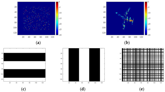
Figure 8.
(a) Label image of a test sample. (b) RD image of the Yak-42 aircraft with complete data and high SNR. (c) Data missing pattern of the incomplete range data. (d) Data missing pattern of the incomplete azimuth data. (e) Data missing pattern of the 2D incomplete data.
In the training stage, the adjustable parameters are initialized as and . In addition, the piecewise linear function is initialized as a soft threshold function with , and the control points are equally spaced with . Then, the 2D-ADN is trained following Section 4.2, and the number of stages is set to 7 according to (40).
For the simulated test data, we fed the test samples into the trained 2D-ADN, and calculated the NMSE, the peak signal-to-noise ratio (PSNR), the structure similarity index measure (SSIM), and the entropy of the image (ENT) according to the output and the label for quantitative performance evaluation. In addition, we compared the imaging results of the 2D-FISTA, untrained 2D-ADN, UNet [32], and trained 2D-ADN. In particular, as a data-driven method, the UNet has much more trainable parameters than the 2D-ADN. To avoid overfitting, we generated 1000 samples as the simulated data set, where 800 samples constituted the training set and the rest constituted the test set. The network was trained by 28 epochs, and the training time was 22 min. For 2D-ADN, the training terminated when the relative error of the loss fell below , and the training time was 19 min. For 2D-FISTA, the parameters were initialized as and the algorithm terminated when the image NMSE in adjacent iterations fell below .
Additionally, we fed the measured data of a Yak-42 aircraft with random phase errors into the trained 2D-ADN and obtained the high-resolution imaging in various observation conditions. The original RD image with complete data and high SNR is shown in Figure 8b. The algorithm terminated when the NMSE between adjacent iterations fell below .
The imaging results were obtained with MATLAB coding without optimization, using an Intel i9-10920X 3.50-GHz computer with a 12-core processor.
5.1. Complete Data
For the test sample illustrated in Figure 8a, imaging results are shown in Figure 9 and the corresponding metrics are shown in Table 1. It was observed that the image obtained by 2D-FISTA and untrained 2D-ADN are noisy with spurious scattering centers. On the contrary, the image obtained by trained 2D-ADN has the smallest NMSE and ENT, and the highest PSNR and SSIM, demonstrating its superior imaging performance. In addition, 2D-FISTA has the longest running time due to slow convergence. The UNet obtains satisfying denoising performance and has the shortest running time of only 0.01 s.
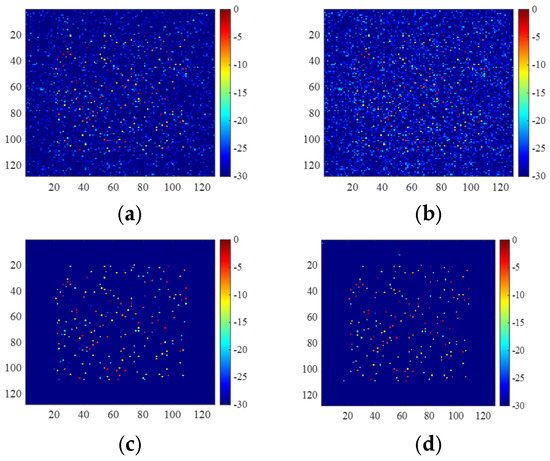
Figure 9.
Images of the complete data obtained by (a) 2D-FISTA, (b) untrained 2D-ADN, (c) UNet, and (d) trained 2D-ADN.

Table 1.
Quantitative performance evaluation for the complete simulation data.
For measured data of the Yak-42 aircraft, imaging results are shown in Figure 10 and the corresponding entropies and running times are shown in Table 2. Compared with the available methods, the trained 2D-ADN obtained better-focused images with a clearer background. In addition, the running time increased because 2D-ADN was implemented multiple times for phase error estimation. The untrained 2D-ADN had the longest running time since the strong background noise hindered fast convergence.
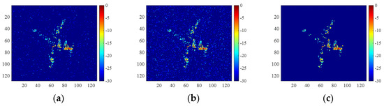
Figure 10.
Yak-42 images of complete data obtained by (a) 2D-FISTA, (b) untrained 2D-ADN, and (c) trained 2D-ADN.
Table 2.
Quantitative performance evaluation for the complete measured data.
5.2. Incomplete Range Data
The data missing pattern of the incomplete range data is shown in Figure 8c, where the white bars denote the available echoes and the black ones denote the missing echoes.
For the same test sample, the reconstruction results are shown in Figure 11, and the metrics for quantitative comparison are shown in Table 3. Still, the trained 2D-ADN demonstrated the best reconstruction performance.
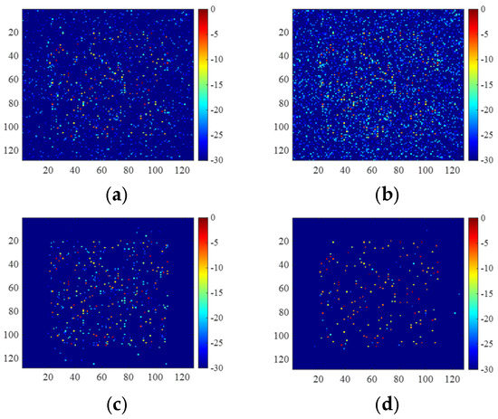
Figure 11.
Images of the incomplete range data with data missing pattern shown in Figure 8c, which are obtained by (a) 2D-FISTA, (b) untrained 2D-ADN, (c) UNet, and (d) trained 2D-ADN.
Table 3.
Quantitative performance evaluation for the incomplete range simulation data.
For the same measured data of the Yak-42 aircraft, the reconstruction results are shown in Figure 12, where the trained 2D-ADN generated better-focused images with a clearer background than other methods. The corresponding entropies and running times are shown in Table 4, where 2D-FISTA has the longest time.
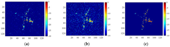
Figure 12.
Yak-42 images of the incomplete range data obtained by (a) 2D-FISTA, (b) untrained 2D-ADN, and (c) trained 2D-ADN.
Table 4.
Quantitative performance evaluation for the incomplete range measured data.
5.3. Incomplete Azimuth Data
The data missing pattern of the incomplete azimuth data is shown Figure 8d. For the same test sample, the reconstruction results are shown in Figure 13, and the metrics for quantitative comparison are shown in Table 5.
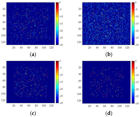
Figure 13.
Images of the incomplete azimuth data with data missing pattern shown in Figure 8d, which are obtained by (a) 2D-FISTA, (b) untrained 2D-ADN, (c) UNet, and (d) trained 2D-ADN.
Table 5.
Quantitative performance evaluation for the incomplete azimuth simulation data.
For the same measured data, the imaging results are shown in Figure 14, and the corresponding entropies and running times are shown in Table 6. Similarly, 2D-ADN achieved well-focused imaging with the shortest running time.
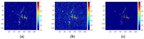
Figure 14.
Yak-42 images of the incomplete azimuth data obtained by (a) 2D-FISTA, (b) untrained 2D-ADN, and (c) trained 2D-ADN.
Table 6.
Quantitative performance evaluation for the incomplete azimuth measured data.
5.4. 2D Incomplete Data
The data missing pattern of the 2D incomplete data is shown in Figure 8e. For the same test sample, the reconstruction results are shown in Figure 15, and the metrics for the quantitative comparison are shown in Table 7.
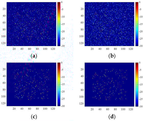
Figure 15.
Images of the 2D incomplete data with data missing pattern shown in Figure 8e, which are obtained by (a) 2D-FISTA, (b) untrained 2D-ADN, (c) UNet, and (d) trained 2D-ADN.
Table 7.
Quantitative performance evaluation for the 2D incomplete simulation data.
For the same measured data, the reconstruction results are shown in Figure 16, and the corresponding metrics are shown in Table 8, which demonstrate the superiority of 2D-ADN over the other available methods under complex observation conditions.
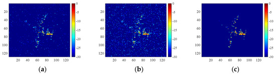
Figure 16.
Yak-42 images of the 2D incomplete data obtained by (a) 2D-FISTA, (b) untrained 2D-ADN, and (c) trained 2D-ADN.
Table 8.
Quantitative performance evaluation for the 2D incomplete measured data.
6. Discussion
6.1. Influence of the Data Loss Rate and SNR
To further analyze the reconstruction performance of the proposed method, we designed more experiments using only 25% and 10% of the available data, where the SNRs were set to 0 dB, 5 dB, and 10 dB, respectively. The imaging results are shown in Figure 17 and Figure 18. The corresponding metrics are shown in Table 9 and Table 10.
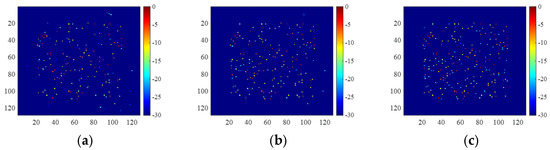
Figure 17.
Images generated using 25% of available data with SNRs of (a) 0 dB, (b) 5 dB, and (c) 10 dB.
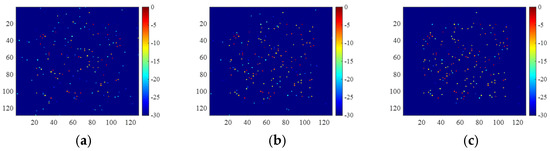
Figure 18.
Images generated using 10% of available data with SNRs of (a) 0 dB, (b) 5 dB, and (c) 10 dB.
Table 9.
Quantitative performance evaluations using 25% available data.
Table 10.
Quantitative performance evaluations using 10% available data.
It was observed that the imaging quality degraded heavily with the decrease of the available data for SNR of 0 dB. If we raised the SNR to 5 dB or 10 dB, however, the imaging performance improved rapidly. Therefore, the SNR has a greater impact on the imaging quality than the data loss rate. Furthermore, although it inherits the reconstruction performance of 2D-ADMM and utilizes a more flexible piecewise linear function as the denoiser, the 2D-ADN is still sensitive to low SNR.
6.2. Choice of the Optimal Regularization Parameter
In 2D-ADMM, it is necessary to perform multiple manual adjustments of the regularization parameter and penalty parameter to obtain the best results. In addition, the adjustable parameters of the 2D-ADMM are fixed during iteration, which lacks flexibility. On the contrary, the 2D-ADN learns the optimal parameters of each layer separately, thus having more flexibility and a better reconstruction performance than the 2D-ADMM.
For a data loss rate of 50% and an SNR of 0dB, we obtained the optimal parameters with the minimum NSME by manual tuning, i.e., and . Imaging results of the optimal 2D-ADMM are shown in Figure 19 and Table 11. It was observed that the quality of the 2D-ADN image was better than the 2D-ADMM image obtained by parameter tuning.
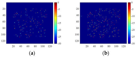
Figure 19.
Images obtained by (a) optimal 2D-ADMM and (b) trained 2D-ADN.
Table 11.
Quantitative performance evaluation for different methods.
6.3. Difference Between 2D-ADMM and 2D-ADN
Through the use of the unrolling method, 2D-ADN deviates from the original 2D-ADMM algorithm. Figure 20 shows the variations of NMSE for 2D-ADMM and 2D-ADN, respectively. Figure 21 shows the outputs of each stage for 2D-ADN. It was observed that the NMSE of the 2D-ADMM gradually decreased; while the NMSE of the 2D-ADN fluctuated and then reached the minimum. Therefore, end-to-end training guarantees the rapid dropping of NMSE, and the flexible network structure boosts the reconstruction performance.
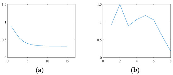
Figure 20.
NMSE of (a) 2D-ADMM and (b) 2D-ADN.
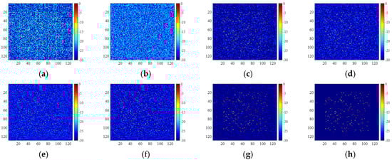
Figure 21.
Images of 2D-ADN at different stages: (a) , (b) , (c) , (d) , (e) , (f) , (g) , (h) .
7. Conclusions
This article proposed 2D-ADN for high-resolution 2D ISAR imaging and autofocusing under complex observational environments. Firstly, the 2D mapping from the ISAR images to echoes in the wavenumber domain was established. Then, iteration formulae based on the 2D-ADMM were derived for high-resolution ISAR imaging and, combined with the phase error estimation method, an imaging and autofocusing method was proposed. On this basis, the 2D-ADMM was generalized and unrolled into an -stage 2D-ADN, which consisted of reconstruction layers, nonlinear transform layers, and multiplier update layers. The 2D-ADN effectively tackles the parameter adjustment problem of model-driven methods and possesses more interpretability than data-driven methods. Experiments have shown that after the end-to-end training by randomly generated samples off-line, the 2D-ADN achieves the better-focused 2D imaging of measured data with random phase errors than the available methods while maintaining computational efficiency.
Future work will be focused on designing network architectures which incorporate residual translational motion compensation and 2D imaging, and on designing noise and jamming-robust network architectures in a Bayesian framework.
Author Contributions
X.L. proposed the method, designed the experiment, and wrote the manuscript; X.B. and F.Z. revised the manuscript. All authors have read and agreed to the published version of the manuscript.
Funding
This paper was funded in part by the National Natural Science Foundation of China under Grant No. 61971332, 61801344, and 61631019.
Conflicts of Interest
The authors declare no conflict of interest.
References
- Kang, L.; Luo, Y.; Zhang, Q.; Liu, X.-W.; Liang, B.-S. 3-D Scattering Image Sparse Reconstruction via Radar Network. IEEE Trans. Geosci. Remote Sens. 2020. [Google Scholar] [CrossRef]
- Bai, X.R.; Zhou, X.N.; Zhang, F.; Wang, L.; Zhou, F. Robust pol-ISAR target recognition based on ST-MC-DCNN. IEEE Trans. Geosci. Remote Sens. 2019, 57, 9912–9927. [Google Scholar] [CrossRef]
- Carrara, W.G.; Goodman, R.S.; Majewski, R.M. Spotlight Synthetic Aperture Radar: Signal Processing Algorithms; Artech House: Boston, MA, USA, 1995; Chapter 2. [Google Scholar]
- Zhao, L.F.; Wang, L.; Yang, L.; Zoubir, A.M.; Bi, G.A. The race to improve radar imagery: An overview of recent progress in statistical sparsity-based techniques. IEEE Signal Process. Mag. 2016, 33, 85–102. [Google Scholar] [CrossRef]
- Bai, X.R.; Zhang, Y.; Zhou, F. High-resolution radar imaging in complex environments based on Bayesian learning with mixture models. IEEE Trans. Geosci. Remote Sens. 2019, 57, 972–984. [Google Scholar] [CrossRef]
- Li, R.Z.; Zhang, S.H.; Zhang, C.; Liu, Y.X.; Li, X. Deep Learning Approach for Sparse Aperture ISAR Imaging and Autofocusing Based on Complex-Valued ADMM-Net. IEEE Sens. J. 2021, 21, 3437–3451. [Google Scholar] [CrossRef]
- Shao, S.; Zhang, L.; Liu, H.W. High-Resolution ISAR Imaging and Motion Compensation With 2-D Joint Sparse Reconstruction. IEEE Trans. Geosci. Remote Sens. 2020, 58, 6791–6811. [Google Scholar] [CrossRef]
- Kang, M.; Lee, S.; Lee, S.; Kim, K. ISAR imaging of high-speed maneuvering target using gapped stepped-frequency waveform and compressive sensing. IEEE Trans. Image Process. 2017, 26, 5043–5056. [Google Scholar] [CrossRef]
- Hu, P.J.; Xu, S.Y.; Wu, W.Z.; Chen, Z.P. Sparse subband ISAR imaging based on autoregressive model and smoothed algorithm. IEEE Sens. J. 2018, 18, 9315–9323. [Google Scholar] [CrossRef]
- Beck, A.; Teboulle, M. A fast iterative shrinkage-thresholding algorithm for linear inverse problems. SIAM J. Imag. Sci. 2009, 2, 183–202. [Google Scholar] [CrossRef]
- Li, S.; Amin, M.; Zhao, G.; Sun, H. Radar imaging by sparse optimization incorporating MRF clustering prior. IEEE Geosci. Remote Sens. Lett. 2020, 17, 1139–1143. [Google Scholar] [CrossRef]
- Afonso, M.V.; Bioucas-Dias, J.M.; Figueiredo, M.A.T. Fast image recovery using variable splitting and constrained optimization. IEEE Trans. Image Process. 2010, 19, 2345–2356. [Google Scholar] [CrossRef]
- Bai, X.R.; Zhou, F.; Hui, Y. Obtaining JTF-signature of space-debris from incomplete and phase-corrupted data. IEEE Trans. Aerosp. Electron. Syst. 2017, 53, 1169–1180. [Google Scholar] [CrossRef]
- Bai, X.R.; Wang, G.; Liu, S.Q.; Zhou, F. High-Resolution Radar Imaging in Low SNR Environments Based on Expectation Propagation. IEEE Trans. Geosci. Remote Sens. 2020, 59, 1275–1284. [Google Scholar] [CrossRef]
- Li, S.Y.; Zhao, G.Q.; Zhang, W.; Qiu, Q.W.; Sun, H.J. ISAR imaging by two-dimensional convex optimization-based compressive sensing. IEEE Sens. J. 2016, 16, 7088–7093. [Google Scholar] [CrossRef]
- Hashempour, H.R. Sparsity-Driven ISAR Imaging Based on Two-Dimensional ADMM. IEEE Sens. J. 2020, 20, 13349–13356. [Google Scholar] [CrossRef]
- Pu, W. Deep SAR Imaging and Motion Compensation. IEEE Trans. Image Process. 2021, 30, 2232–2247. [Google Scholar] [CrossRef]
- Pu, W. Shuffle GAN with Autoencoder: A Deep Learning Approach to Separate Moving and Stationary Targets in SAR Imagery. IEEE Trans. Neural Netw. Learn. Syst. 2021. [Google Scholar] [CrossRef]
- Hu, C.Y.; Wang, L.; Li, Z.; Sun, L.; Loffeld, O. Inverse synthetic aperture radar imaging using complex-value deep neural network. J. Eng. 2019, 2019, 7096–7099. [Google Scholar] [CrossRef]
- Zhang, J.; Ghanem, B. ISTA-Net: Interpretable optimization-inspired deep network for image compressive sensing. In Proceedings of the IEEE Conference on Computer Vision and Pattern Recognition, Salt Lake City, UT, USA, 19–21 June 2018; pp. 1828–1837. [Google Scholar]
- Ramírez, J.M.; Torre, J.I.M.; Fuentes, H.A. LADMM-Net: An Unrolled Deep Network for Spectral Image Fusion from Compressive Data. 2021. Available online: https://arxiv.org/abs/2103.00940 (accessed on 10 June 2021).
- Monga, V.; Li, Y.; Eldar, Y.C. Algorithm Unrolling: Interpretable, Efficient Deep Learning for Signal and Image Processing. IEEE Signal Process. Mag. 2021, 38, 18–44. [Google Scholar] [CrossRef]
- Hu, C.Y.; Li, Z.; Wang, L.; Guo, J.; Loffeld, O. Inverse synthetic aperture radar imaging using a Deep ADMM Network. In Proceedings of the 20th International Radar Symposium (IRS), Ulm, Germany, 26–28 June 2019; pp. 1–9. [Google Scholar]
- Qiu, W.; Zhao, H.; Zhou, J.; Fu, Q. High-resolution fully polarimetric ISAR imaging based on compressive sensing. IEEE Trans. Geosci. Remote Sens. 2014, 52, 6119–6131. [Google Scholar] [CrossRef]
- Liu, L.; Zhou, F.; Tao, M.L.; Sun, P.G.; Zhang, Z.J. Adaptive translational motion compensation method for ISAR imaging under low SNR based on particle swarm optimization. IEEE J. Sel. Top. Appl. Earth Obs. Remote Sens. 2015, 8, 5146–5157. [Google Scholar] [CrossRef]
- Wang, Y.; Yang, J.; Yin, W.; Zhang, Y. A new alternating minimization algorithm for total variation image reconstruction. SIAM J. Imag. Sci. 2009, 1, 248–272. [Google Scholar] [CrossRef]
- Combettes, P.; Wajs, V. Signal recovery by proximal forward-backward splitting. Siam J. Multiscale Modeling Simul. 2005, 4, 1168–1200. [Google Scholar] [CrossRef]
- Zhao, L.; Wang, L.; Bi, G.A.; Yang, L. An autofocus technique for high-resolution inverse synthetic aperture radar imagery. IEEE Trans. Geosci. Remote Sens. 2014, 52, 6392–6403. [Google Scholar] [CrossRef]
- Sun, J.; Li, H.B.; Xu, Z.B. Deep ADMM-Net for compressive sensing MRI. In Proceedings of the 30th International Conference on Neural Information Processing Systems, Barcelona, Spain, 5–10 December 2016; pp. 10–18. [Google Scholar]
- Yang, Y.; Sun, J.; Li, H.B.; Xu, Z.B. ADMM-CSNet: A deep learning approach for image compressive sensing. IEEE Trans. Pattern Anal. Mach. Intell. 2020, 42, 521–538. [Google Scholar] [CrossRef] [PubMed]
- Petersen, K.B.; Pedersen, M.S. The Matrix Cookbook; Version 20121115; Technical University of Denmark: Copenhagen, Denmark, 2012; p. 24. Available online: http://www2.compute.dtu.dk/pubdb/pubs/3274-full.html (accessed on 10 June 2021).
- Yang, T.; Shi, H.Y.; Lang, M.Y.; Guo, J.W. ISAR imaging enhancement: Exploiting deep convolutional neural network for signal reconstruction. Int. J. Remote Sens. 2020, 41, 9447–9468. [Google Scholar] [CrossRef]
Publisher’s Note: MDPI stays neutral with regard to jurisdictional claims in published maps and institutional affiliations. |
© 2021 by the authors. Licensee MDPI, Basel, Switzerland. This article is an open access article distributed under the terms and conditions of the Creative Commons Attribution (CC BY) license (https://creativecommons.org/licenses/by/4.0/).