MDCwFB: A Multilevel Dense Connection Network with Feedback Connections for Pansharpening

Abstract

In most practical applications of remote sensing images, high-resolution multispectral images are needed. Pansharpening aims to generate high-resolution multispectral (MS) images from the input of high spatial resolution single-band panchromatic (PAN) images and low spatial resolution multispectral images. Inspired by the remarkable results of other researchers in pansharpening based on deep learning, we propose a multilevel dense connection network with a feedback connection. Our network consists of four parts. The first part consists of two identical subnetworks to extract features from PAN and MS images. The second part is a multilevel feature fusion and recovery network, which is used to fuse images in the feature domain and to encode and decode features at different levels so that the network can fully capture different levels of information. The third part is a continuous feedback operation, which refines shallow features by feedback. The fourth part is an image reconstruction network. High-quality images are recovered by making full use of multistage decoding features through dense connections. Experiments on different satellite datasets show that our proposed method is superior to existing methods, through subjective visual evaluation and objective evaluation indicators. Compared with the results of other models, our results achieve significant gains on the multiple objective index values used to measure the spectral quality and spatial details of the generated image, namely spectral angle mapper (SAM), relative global dimensional synthesis error (ERGAS), and structural similarity (SSIM).

1. Introduction

Remote sensing satellite images are a type of image that has been widely concerned and applied at present. They provide an important reference for applications in digital maps, disaster emergency, and geological observation [1,2]. In practical remote sensing image applications, the images must simultaneously have the highest spatial resolution and spectral resolution. The two most important metrics, the incident radiation energy of the sensor and the amount of data collected by the sensor, are limited by the physical structure of the satellite sensor, making it impossible to obtain remote sensing images with a high spatial resolution and spectral resolution at the same time.

To address this problem, current Earth observation satellites generally use two different types of sensors simultaneously. They are used to obtain single-band panchromatic (PAN) images with a high spatial resolution, but low spectral resolution, and multi-band spectral (MS) images with complementary characteristics. As far as possible, the information from the two images is used simultaneously, and a pansharpening algorithm is typically used to fuse the two images so as to obtain images with both a high spatial resolution and high spectral resolution.

Because of the demand for high-quality remote sensing images, much pansharpening-based work has been carried out, and various algorithms for remote sensing image fusion have been proposed, namely: (1) component substitution (CS) [3,4,5,6], (2) multi-resolution analysis (MRA) [7,8,9,10,11], (3) hybrid methods [12,13], and (4) model-based algorithms [14,15,16]. The core idea of the CS method is to first rely on conversion to project MS images into another space to separate the spatial structure and the spectral information. The PAN image and spatial structure component are then matched and replaced by the histogram so that the PAN image has the same mean value and equation as the replaced component, and finally, the pansharpening task is completed by an inverse transformation operation. Methods such as intensity-hue-saturation (IHS) [3], principal component analysis (PCA) [4], Gram–Schmidt (GS) [5], and partial substitution (PRACS) [6] all adopt this concept. These methods achieve good results when the PAN image and MS image are highly correlated, but because of the local differences caused by a spectral mismatch between the PAN image and MS image, there is obvious spectral distortion in the fusion results.

In the MRA method, three main steps are used to fuse the image. The first step is to use the pyramid transform or wavelet transform to process the source image and divide it into multiple scales. Then, the fusion of each scale of the source image is carried out, and the inverter operation generates the fusion result. This method provides both spatial and frequency domain localisation. Decimated wavelet transform [7], à trous wavelet transform [8], Laplacian Pyramid [9], Contourlet [10], and Curvelet [11] are examples of this approach.

The hybrid method combines the advantages of CS and MRA methods in a combination of ways to achieve higher-performance fusion results. Model-based algorithms operate mainly by establishing the MS image, PAN image, and high-resolution multispectral (HRMS) image relationship model. They rely on prior knowledge for image fusion. A hierarchical Bayesian model to fuse many multi-band images with various spectral and spatial resolutions is proposed in [14]. An online coupled dictionary learning (OCDL) [15], and, in [16], two fusion algorithms by incorporating the contextual constraints via MRF models into the fusion model, have been proposed.

In recent years, deep learning and convolutional neural networks have achieved outstanding results in all fields of image processing [17,18,19,20,21,22,23,24,25,26,27,28,29,30,31,32]. Inspired by image super-resolution using deep convolutional neural networks (SRCNN) [17,18], Masi et al. [19] proposed a network called pansharpening by convolutional neural networks (PNN), which adopts the same three-layer structure as the other and combines specific knowledge in the field of remote sensing to introduce nonlinear radiation indicators so as to increase the input. This was the first application of a CNN in the pansharpening field. With the remarkable effect of the residual structure, Wei et al. [20] designed a deep residual network (DRPNN) for pansharpening. He et al. [21] proposed two detail-based networks to clarify the role of CNN in pansharpening tasks from a theoretical perspective, and clearly explained the effectiveness of the residual structures for pansharpening.

Yang et al. [22] proposed a deep network architecture for pansharpening (PanNet), which is different from the other methods. A hopping connection called spectral mapping was used to compensate for spectral loss caused by training in the high-pass domain. This approach has achieved remarkable results, but it still has significant limitations. It is generally accepted that PAN and MS images contain different information. The PAN image is a carrier of geometric detail (spatial) information, while the MS image preserves spectral information. PanNet is trained by directly superimposing the PAN and MS image input network, resulting in the network’s inability to fully extract the different features contained in the PAN and MS images, and results in an insufficient use of different spatial information and spectral information. It only uses a simple residual structure, which cannot fully extract the image features of different scales, and lacks the ability to recover details. The network directly outputs the fusion results through one convolutional layer, and fails to make full use of all of the features extracted by the network, affecting the final fusion effect.

In this paper, we propose a multilevel dense connection network with feedback connections (MDCwFB), including two branches, a detail branch, and an approximate branch, based on the idea of detail injection and super-resolution work. Different spatial and spectral information are extracted from PAN images and MS images by the dual-stream structure. Multi-scale blocks with attention mechanisms are used on both lines to extract more abundant and effective multi-scale features from the image. The image fusion and reconstruction work are carried out in the feature domain. The fused features are encoded and decoded based on the idea of a dense connection. The shallow network is limited by the size of the receptive field, and can only extract rough features; however, these features are repeatedly used in the subsequent network, which further limits the learning ability of the network. Therefore, we introduce the feedback connection mechanism to transfer the deep features back to the shallow network through a long jump connection, which is used to optimise the rough low-level features and enhance the early reconstruction ability of the network. Through the interaction between the PAN image and MS image features, the detail branch can fully extract the details of the low-resolution multispectral (LRMS) image supplemented as an approximate branch, and the two can help each other obtain an excellent HRMS image.

In summary, the main contributions of this study are as follows:

• We propose a multi-scale feature extraction block with an attention mechanism (MEBwAM) to solve the problems of insufficient feature extraction and the lack of multi-scale feature extraction ability of PAN images and MS images using multiple depth cascaded networks. The spatial information and channel information are compressed separately to obtain an importance index.
• We use multilevel coding and decoding combined with densely connected structures to fuse and reconstruct the extracted spatial and spectral information in the feature domain. Deep networks encode the language and abstract information of the images, making it difficult to recover the texture, boundary, and color information from the advanced features; however, shallow structures are very good at identifying these details. We inject low-level features into high-level features through long jump connections, which can more easily recover fine realistic images, and dense connections to make the feature graph semantic level in the encoder closer to the feature graph in the decoder.
• We propose using multiple subnetworks. We iterate the deep structure in the subnetwork to inject the deep features from the previous subnetwork, that is, the HRMS that completes rough reconstruction, into the shallow structure of the latter subnetwork. This is done by way of a feedback connection to optimize the shallow features of the latter, enabling the network to obtain a better reconstruction ability earlier.
• We use the L₁ loss function to optimise the network and attach the loss function to each subnet to monitor its output in order to ensure that useful information can be transmitted backwards in each iteration.

The remainder of this paper is arranged as follows. We present the CNN background knowledge and work that has achieved remarkable results in other areas and other related work based on CNN pansharpening in Section 2. Section 3 introduces the motivation of our proposed multilevel dense connected network with a feedback connection, and explains the structure of each part of the network in detail. In Section 4, we show the experimental results and compare them with the other methods. We discuss the effectiveness of the network structure in Section 5, and we summarise the paper in Section 6.

2. Background and Related Work

2.1. Convolutional Neural Networks

VGG-Net [25] and GoogLe-Net [26] show the possibility of obtaining better results by increasing the depth and width of the network. Using multiple continuous small-size instead of large-size convolution kernels to reduce the network parameters and using different-size convolution kernels to obtain multi-scale features will inspire the design of CNN frames in the future.

Previous work has shown that increasing the depth of the network improves the performance of the network significantly, but because of the gradient explosion and gradient disappearance, deeper networks are difficult to train. He et al. [27] proposed a residual learning framework to reduce the difficulty of network optimisation and to reduce degradation problems so that deeper network structures could be used. ResNet, a method of fast identity mapping, is used to design residual blocks; adding shortcut connections between the input and output neither introduces additional parameters nor increases computational complexity. Simply learning the difference between input and output makes network optimisation simple, allowing for the design of deeper and more complex network structures to improve the results. However, even when dealing with a minimal dataset, it is easy to result in network overfitting. To overcome this difficulty, Huang et al. [28] proposed the dense connection network (DenseNet), designed for all of the previous layers and the rear layers, which has excellent protection against overfitting. DenseNet makes comprehensive use of simple features from shallow networks through feature reuse, and achieves a better performance than ResNet, with fewer parameters and lower computational costs.

Olaf et al. [29] proposed the U-Net network, which has a fully symmetric encoder-decoder structure. The compression path in the first half is used for feature extraction, and the symmetric extended path is used for image recovery. The encoder acquires the multi-scale features by reducing the spatial dimension, and the decoder gradually recovers the details and spatial dimensions of the image. The loss of information during the downsampling process is compensated by adding a shortcut connection between the encoder and the decoder, which helps the decoder to better repair the details of the target. This concept is widely used by other computer vision and image processing tasks. Inspired by the idea that humans choose the next picture according to pictures they have already seen, Li et al. [32] proposed a picture super-resolution feedback network to refine the low-level information through high-level information. The design concept of these image processing network frameworks has inspired other researchers who carried out the pansharpening task and promoted the development of the convolutional neural network and specific knowledge for pansharpening work in the remote sensing field.

2.2. CNN-Based Pansharpening

Inspired by the remarkable results of image super-resolution work based on CNNs, Masi et al. [19] first proposed using a CNN to complete the pansharpening task. The MS image and PAN image channels are superimposed into the network to obtain a form similar to the SRCNN single input and single output. In a follow-up work, a nonlinear radiation index was introduced to increase the input and further improve performance. Wei et al. [20] introduced a residual network into the pansharpening work and designed a deep residual network with an 11-layer network. Traditional pansharpening methods generally use the high-pass information contained in PAN images to enhance the structural consistency. Inspired by this concept, Yang et al. [22] proposed a network called PanNet, which combines knowledge and deep learning technology in the remote sensing field. It uses high-pass components as the network input. Before entering the network, the original image is used to subtract the low-pass content obtained using the mean filter so as to obtain the high-frequency information of the MS and PAN images used for training. To compensate for the loss of spectral information caused by obtaining high-frequency information in the early stage, PanNet uses a jump connection called spectral mapping to inject the up-sampled MS image into the fusion image. Enhancing the spatial information capture ability and forcing the network to fuse spectral information through the high-frequency information training network delivers excellent results. To further improve the network performance, Fu et al. [33] introduced cavity convolution based on PanNet. By using multi-scale expansion blocks with convolution layers with different expansion rates, the ability of the network to fully capture the multi-scale features of the PAN images and MS images is enhanced, and high-precision fusion images are obtained. The above networks use the L₂ loss function to optimise the network. Because early work using the L₂ loss function to optimise the network produces image blur, follow-up work uses the L₁ loss function to train the new network.

Liu et al. [34] proposed a two-stream fusion network for pansharpening tasks. Because PAN and MS images have different spatial and spectral information features, TFNet uses a two-stream structure to extract features from the PAN and MS images, respectively. The image fusion reconstruction task is completed in the feature domain through the encoder–decoder structure. Fu et al. [35] proposed an improvement to TFNet called ResTFNet, in which a basic residual structure to improve the network performance replaces the common CNN unit used by the former. Fu et al. [36] proposed a generation countermeasure network for remote sensing image pansharpening (PSGAN) using a two-stream structure to extract complementary information from the MS and PAN images. A generator is then built to produce high-quality HRMS images using encoders and decoders. In PSGAN and RED-cGAN [37], which are GAN-based models, the generator tries to generate images similar to the ground truth and the discriminator tries to distinguish between the generated images and the HRMS images. In RED-cGAN, the results are further improved by introducing the residual encoder–decoder network and conditional GAN. So, both the generator and the discriminator network in these two methods need the HRMS images for supervised learning. The two models are different from other methods, and during training, they use multiple loss functions to constrain network learning.

3. Proposed Network

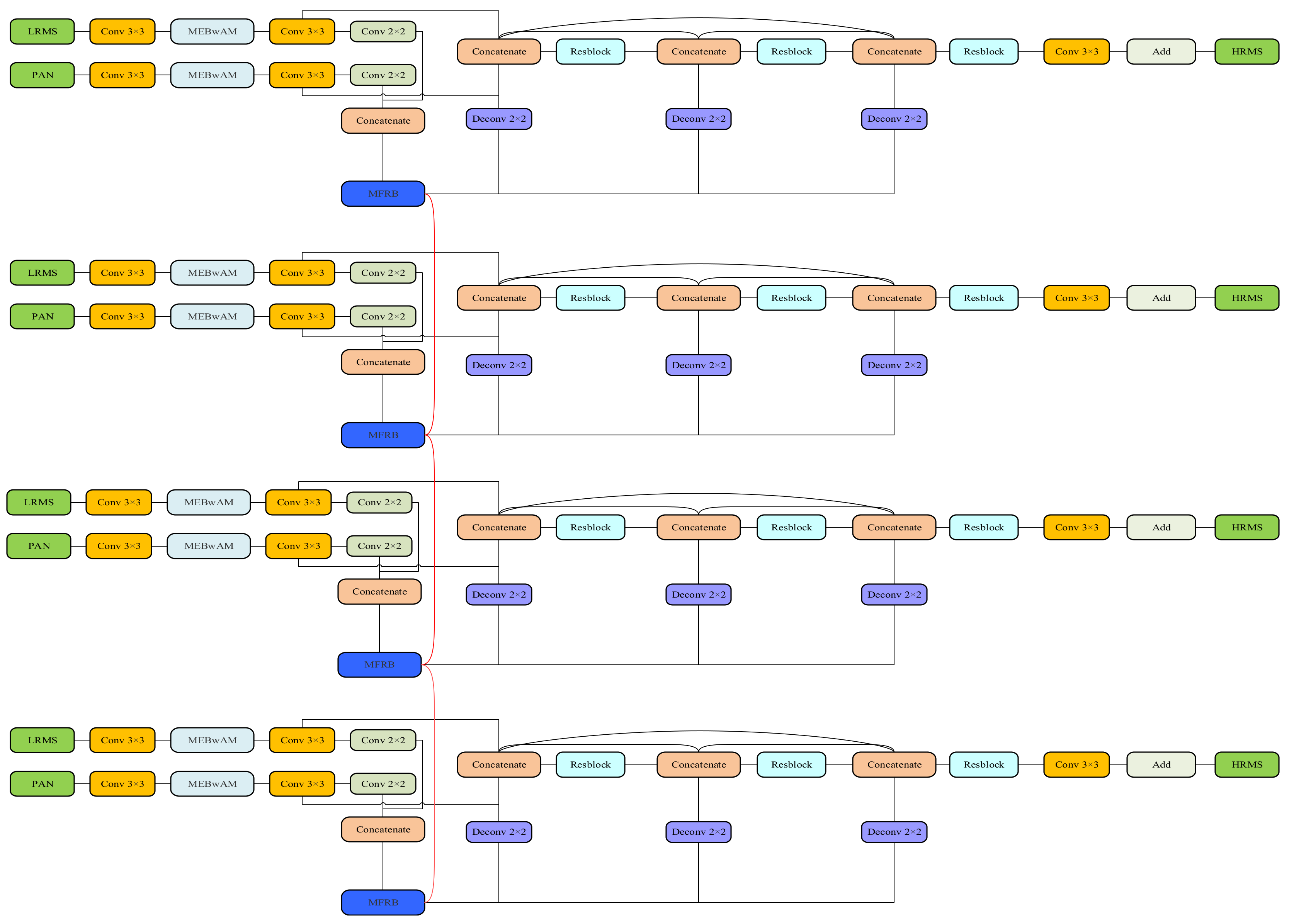
In this section, we will introduce in detail the specific structure of the MDCwFB model proposed in this study, which not only has a clear interpretability, but also has an excellent ability to prevent overfitting and to reconstruct images early. We will introduce the algorithm solution for the proposed model and give a detailed description of each part of the network framework. The schematic framework of our proposed network is shown in Figure 1 and Figure 2. It can be seen that our model includes two branches: one, the merely approximate branch of the LRMS graph, enhances the retention of spectral information, and the other is the detail branch for extracting spatial details. Such a structure has a clear physical interpretability and reduces uncertainty in the network training. The detail branch, which has a structure similar to the encoder–decoder system, consists of four parts: feature extraction, feature fusion and recovery, feedback connection, and image reconstruction.

3.1. Feature Extraction Networks

A PAN image is considered the carrier of spatial detail in the pansharpening task, and the MS image is the carrier of spectral information. Spatial and spectral information are combined to generate high-resolution images through the PAN and MS image interaction. Based on the ideas described previously, we rely on a CNN to fully extract the different spatial and spectral information and to complete the feature fusion reconstruction and image restoration in the feature domain.

We use two networks with the same structure to extract features from the PAN and MS images, respectively. One network takes a single-band PAN image (size H × W) as the input, and the other takes a multi-band MS image (size H×W×N) as the input. Before entering the network, we upsampled the MS image to the same size as the PAN image via transposing convolution. Each feature extraction subnet consists of two separate convolution layers, followed by a parameter rectified linear unit (PReLU).

Many studies on the CNN framework indicate that the depth and width of the network significantly affect the quality of the results. A deeper and wider network structure can help the network learn richer feature information and can capture the mapping between the semantic information and context information in features. He et al. [26] proposed a residual network structure, and Szegedy et al. [27] proposed an inception network structure that significantly increased the depth and width of the network. The jump connection proposed by the former reduces the training difficulty after the network deepens. The latter points out the direction for the network to extract multi-scale features.

Inspired by the multi-scale expansion blocks proposed by the above work and Yang et al. [33] in PanNet, and the spatial and channel extrusion and excitation blocks proposed by Roy et al. [38] to extract more fully the different-scale features in the image and enhance the more important parts of the features for pansharpening tasks, we propose an MEBwAM to use different receptive fields on a monolayer network and to add to the middle of two convolution layers. The first 3 × 3 convolution layer preliminarily extracts the image features. The second 3 × 3 convolution layer preliminarily fuses the enhanced features of the two branches.

This MEBwAM structure is shown in Figure 3. We did not use cavity convolution to extract multi-scale features, even if it can arbitrarily expand the receptive field without introducing additional parameters. Because of the grid effect, cavity convolution is a sparse sampling method. The superposition of the cavity convolution with multiple different scales causes some features to be unused. Thus, the extracted features will also lose their correlation and continuity of information, which will affect the feature fusion reconstruction. We use convolution kernels of size 3 × 3, 5 × 5, 7 × 7, and 9 × 9 in four branches, respectively. To reduce the high computational cost, we used multiple cascading size 3 × 3 convolution layers to replace the large-size convolution kernels in the other three branches. Each convolution layer is followed by a PReLU. Finally, the results after the four path cascades are fused through one 1 × 1 convolution layer. We then extract the spatial attention and channel attention through two branches and recalibrate the extracted multi-scale features using the obtained indexes to measure the importance. The information that is more important to the fusion results is enhanced, and the relatively invalid parts are suppressed. The channel attention branch uses the global average pooling layer to compress the spatial characteristics, and it combines the 1 × 1 convolution layer and PReLU function to obtain more nonlinearity and better fit the complex correlation between channels. The spatial attention branches use 1 × 1 convolutional layers to compress the channel features. At the end, the two branches use the sigmoid function to obtain an index to measure the spatial information and the importance of the channel, and the jump connection of the whole module effectively reduces the training difficulty and the possible degradation problem, as follows:

$$F_{CSE}(x)=\mathsf{\sigma }(Con{v}_{1,64}(\mathsf{\delta }(Con{v}_{1,32}(\mathsf{\mu }(x)))))$$

(1)

$$F_{SSE}(x)=\mathsf{\sigma }(Con{v}_{1,1}(x))$$

(2)

$$F_{MFRB}=F_{CSE}(x)\ast x+F_{SSE}(x)\ast x+x$$

(3)

$$f_{MS}=Con{v}_{3,64}(\mathsf{\delta }(F_{MFRB}(\mathsf{\delta }(Con{v}_{3,64}(I_{LRMS})))))$$

(4)

$$f_{Pan}=Con{v}_{3,64}(\mathsf{\delta }(F_{MFRB}(\mathsf{\delta }(Con{v}_{3,64}(I_{Pan})))))$$

(5)

$$f_{P+M}=Con{v}_{2,64}(f_{MS})\otimes Con{v}_{2,64}(f_{Pan})$$

(6)

We use $Con{v}_{f,n}(\cdot )$ to represent convolution layers with size f × f convolution kernels and n channels, and $\mathsf{\sigma }(\cdot )$, $\mathsf{\delta }(\cdot )$, and $\mathsf{\mu }(\cdot )$ represent the sigmoid activation functions, PReLU activation function, and global average pooling layer, respectively. LRMS and PAN represent the images as the input, $F_{MFRB}$ represents the multi-scale feature extraction layer, and x refers to the feature fused together by four branches. f_MS and f_Pan represent the extracted MS and PAN image features, respectively, and $\otimes$ represents the concatenation operation.

3.2. Multistage Feature Fusion and Recovery Network

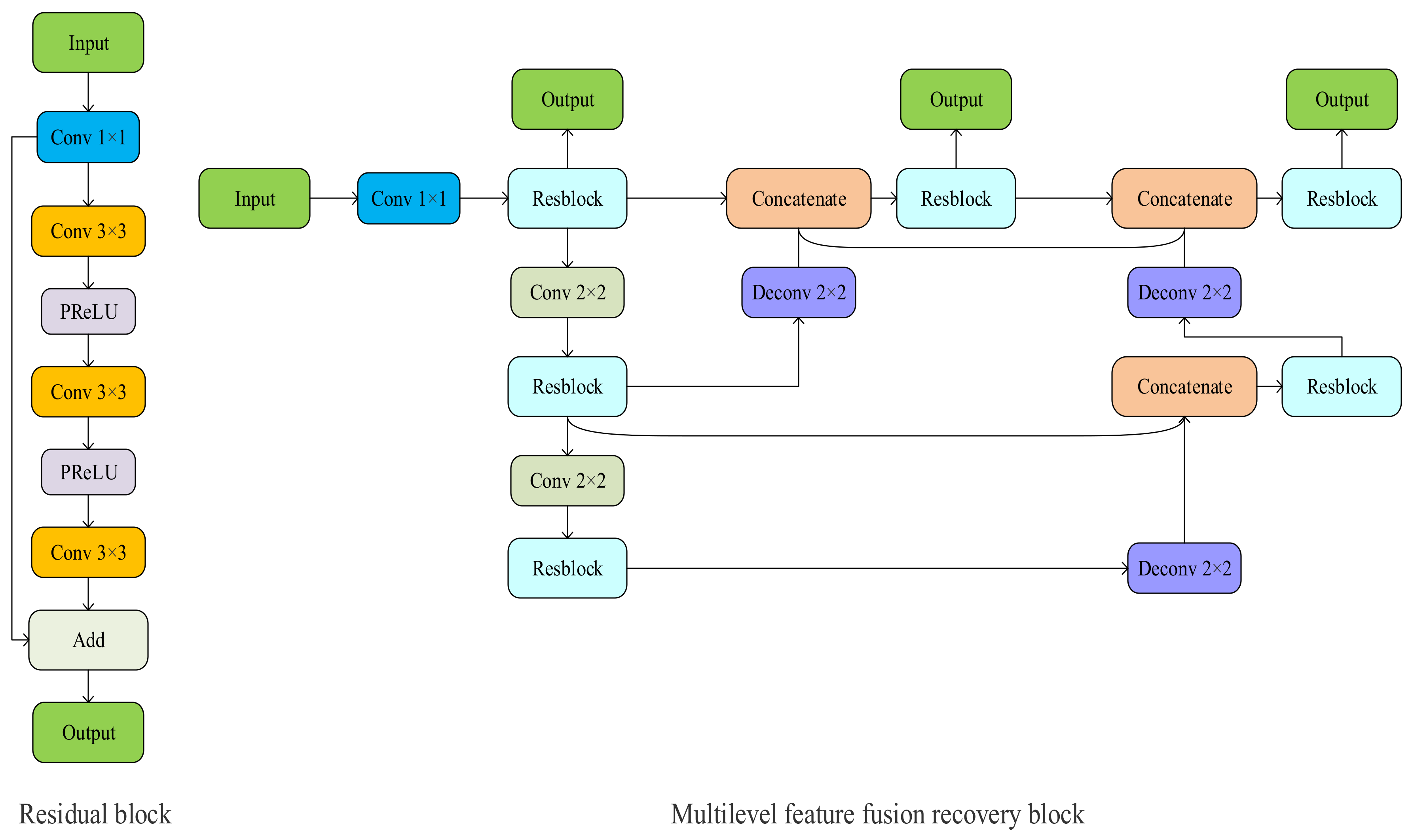
For the encoder–decoder architecture in our proposed network, we propose a multilevel feature fusion recovery block (MFRB) to implement the encoding and decoding operations and subsequent feedback connections. The concrete structures of the MFRB and residual block are shown in Figure 4. We use three residual blocks and two downsampling operations to form the encoder structure. Unlike the symmetric structure of traditional encoder and decoder networks, our decoder structure includes three residual blocks and three upsampling operations. The downsampling operation increases the robustness to some interference of the input image, while obtaining the features of translation invariance, rotation invariance, and scale invariance and reducing the risk of overfitting. Continuous downsampling can increase the size of the receptive field and help the network fully capture multi-scale features. In this study, we choose to use a convolution layer with a step size of two to complete the downsampling operation. The two feature extraction subnets are downsampled after two convolution layers and multi-scale feature extraction blocks.

The structure shown in Figure 4 is inspired by Zhou et al. [39], who proposed the U-Net++ structure for a multilevel feature fusion recovery module. Many studies have shown that because of the different size of the receptive field, the shallow structure focuses on some simple features of the captured image, such as boundary, colour, and texture information. After many convolution operations, the deep structure captures the contextual language information and abstract features of the image. Downsampling operations help the encoder fuse and encode features at different levels, and the features are recovered through upsampling operations and decoders. However, edge information and small parts of large objects are easily lost during multiple downsampling and upsampling operations. It is very difficult to recover detailed texture information from encoded image semantics and abstract information, which seriously affects the quality of the pansharpening. Adding jump connections between encoders and decoders with the same feature map size and using shallow features to help the decoder complete the feature recovery solves this problem to some extent.

Different levels of characteristics focus on different informations, but the importance of the pansharpening tasks is consistent. To obtain higher-precision images, we need to make full use of different levels of features, and simultaneously, we need to solve the problem of using jump connections between the encoder and decoder because of the different feature levels. As shown in Figure 4, we decode the features after each encoding level, which means that our MFRB produces multiple outputs, each corresponding to a feature level. We decode each level of features and then connect the same level of encoder and decoder using a dense connection, which not only makes the feature graph in the encoder and decoder want a closer semantic, level but also increases the ability of the network to resist overfitting. In the network, we double the number of feature graph channels at each downsampling layer and halve the number of feature graph channels at each upsampling layer. The residual blocks in the network include one 1 × 1 convolutional layer and two 3 × 3 convolutional layers. Each convolutional layer is followed by a PReLU. Because we double the number of channels after each downsampling, and the input and output of the residual units need to have the same size, we change the number of channels by 1 × 1 convolutional layers to create hopping connections. The input of each decoder consists of features recovered from the upper decoder and features in the same level of encoder and decoder.

3.3. Feedback Connection Structure

Feedback is the use of one set of conditions to regulate another set of conditions, which is done to increase or suppress changes in the system. The mechanism is called positive feedback when processes tend to increase system changes. Negative feedback refers to processes that try to counter changes and maintain balance. Feedback mechanisms usually exist in human visual systems. In cognitive theory, feedback connections connecting cortical visual regions can transmit response signals from higher-order regions to lower-order regions. Inspired by the work carried out by Li et al. [32] on image super-resolution, they carefully designed a feedback block to extract powerful high-level representations for low-level computer vision tasks and transmit high-level representations to perfect low-level functions. Fu et al. [40] added this feedback connection mechanism for super-resolution tasks to the network of pansharpening tasks. Our proposed network is similar to their network structure with four time steps in the above study, but we use different feedback blocks. We use four identical subnetworks to add feedback connections between adjacent subnetworks. The specific structure of the subnetwork is shown in Figure 2.

Because of the feedforward connection, each network layer can only accept information from the previous layer. The dense connection structure in the subsequent network reuses these features repeatedly, which further limits the network reconstruction ability. The feedback connection solves this problem very well. We complete the initial reconstructed features through the MFRB and input them into the next subnetwork as deep information. This way of bringing high-level information back to the previous layer can supplement the semantic and abstract information lacking in the low-level features, improve the error information carried in the low-level features, and correct some of the previous states so that the network has a solid ability to rebuild early:

$$f_1,f_2,f_3=F_{MFRB}(f_{P+M})$$

(7)

$$f_1,f_2,f_3=F_{MFRB}(f_{P+M}\otimes f_3)$$

(8)

where f₁, f₂, and f₃ represent the three-level features extracted using MFRB, and the subscripts represent the number of downsamplings. The first subnetwork uses only the PAN image and MS image features added after one downsampling as the input to the MFRB structure. The following three subnetworks fuse the recovered feature of the previous subnet and the features of f₃ for the two feature extraction subnets f_P+M, and carry out the subsequent feature fusion recovery work in the input MFRB after the cascade operation represented by the $\otimes$.

3.4. Image Reconstruction Network

For image reconstruction, we use three residual blocks and a convolution layer to process the features after the fusion and recovery operations. Each residual block corresponds to a feature recovered to the original size after upsampling. By adding dense connections between different modules, we use the decoded features from different levels of encoders. Finally, the results of the detail branch are added to the LRMS image, as follows:

$$f_{rb1}=Con{v}_{3,64}(Con{v}_{3,64}(Con{v}_{1,64}(f_{MS}\otimes f_{Pan}\otimes Decon{v}_{2,128}(f_1))))$$

(9)

$$f_{rb2}=Con{v}_{3,64}(Con{v}_{3,64}(Con{v}_{1,64}(f_{MS}\otimes f_{Pan}\otimes f_{rb1}\otimes Decon{v}_{2,128}(f_2))))$$

(10)

$$f_{rb3}=Con{v}_{3,64}(Con{v}_{3,64}(Con{v}_{1,64}(f_{MS}\otimes f_{Pan}\otimes f_{rb1}\otimes f_{rb2}\otimes Decon{v}_{2,128}(f_3))))$$

(11)

$$f_{rb}=Con{v}_{3,4}(f_{MS}\otimes f_{Pan}\otimes f_{rb1}\otimes f_{rb2}\otimes f_{rb3})$$

(12)

$$I_{out}=I_{LRMS}+f_{rb}$$

(13)

We use $\otimes$ to represent cascading operations; and $Decon{v}_{f,n}(\cdot )$ represent convolutional and deconvolutional layers, respectively; and f and n represent the size and number of channels of convolutional kernels, respectively. f_rb1, f_rb2, and f_rb3 restore the multilevel image by reconstructing the three-level features through three residual blocks. Finally, a convolution layer is used to recover the details needed for the LRMS image from the features extracted from the two-stream branches and the reconstructed multilevel image, combined with the LRMS images, and the two branches interact to generate high-precision HRMS images.

3.5. Loss Function

The effectiveness of the network junction is an important factor affecting the final HRMS image quality, while the loss function is another important factor. Early CNN-based pansharpening methods use the L₂ loss function to optimise the network parameters, but the L₂ loss function could give rise to the local minimum value problem and cause artefacts in the flat region. Subsequent studies have proven that the L₁ loss function obtains a better minimum value. Moreover, the L₁ loss function better retains spectral information such as colour and brightness than the L₂ loss function. Hence, the L₁ loss function is chosen to optimise the parameters of the proposed network. We attach the loss function to each subnetwork to monitor the training results while ensuring that the information delivered to the latter subnet in the feedback connection is valid:

$$\mathit{loss}=\frac{1}{N}\sum _{i=1}^N{\left|\Phi (X_p^{(i)},X_m^{(i)};\theta )-Y^{(i)}\right|}_1$$

(14)

where $X_p^{(i)}$, $X_m^{(i)}$, and $Y^{(i)}$ represent a set of training samples; $X_p^{(i)}$ and $X_m^{(i)}$ mean the PAN image and low-resolution MS image, respectively; $Y^{(i)}$ represents high-resolution MS images; $\Phi$ represents the entire network; and $\theta$ is the parameter in the network.

4. Experiments and Analysis

In this section, we will demonstrate the effectiveness and superiority of our proposed method through experiments using the QuickBird, WorldView-2, WorldView-3, and Ikonos datasets. The best model was selected for the experiment by comparing and evaluating the training and test results of models with different network structures and parameters. Finally, the visual and objective indicators of our best model were compared with several other existing traditional algorithms and CNN methods to demonstrate the superior performance of the proposed method.

4.1. Datasets

For QuickBird data, the MS image has four bands, including blue, green, red, and near-infrared (NIR) bands, and a spectral resolution of 450–900 nm. For WorldView-2 and WorldView-3 data, the MS image has eight bands, including coastal, blue, green, yellow, red, edge, NIR, and NIR 2 bands, and the spectral resolutions of the image are 400–1040 nm. For Ikonos data, the MS image has four bands, including blue, green, red, and near NIR bands, and a spectral resolution of 450–900 nm. The spatial resolution information for the different datasets is shown in

Table 1. Spatial resolution and number of bands of datasets for different satellites.

Sensors	Bands	PAN	MS
QuickBird	4	0.61 m	2.44 m
WorldView-2	8	0.46 m	1.85 m
WorldView-3	8	0.31 m	1.24 m
Ikonos	4	1 m	4 m

.

The network architecture in this study was implemented with the Pytorch deep learning framework and was trained on an NVIDIA RTX 2080Ti GPU. The training time for the whole program was about 8 h. We used the Adam optimisation algorithm to minimise the l₁ loss function and optimise the model. We set the learning rate to 0.001, the exponential decay factor to 0.9, and the weight decay to 10⁻⁶. The LRMS and PAN images were both downsampled by the Wald protocol in order to use the original LRMS images as the ground truth images. The image patch size was set to 64 × 64 and the batch size to 64. To facilitate visual observation, the red, green, and blue bands of the multispectral images were used as imaging bands of RGB images to form colour images. The results are presented using ENVI. In the calculation of the image evaluation indexes, other bands of the images were used at the same time. The training set was used to train the network, and the validation set was used to evaluate the performance. The size of the training and test sets for the four datasets is shown in

Table 2. Size of training and test sets for different satellite datasets.

Dataset	Train Set	Validation Set	The Size of the Original PAN
QuickBird	750	200	7472 × 6020
WorldView-2	600	150	8080 × 7484
WorldView-3	1000	300	13,632 × 11,244
Ikonos	144	16	5192 × 4632

.

4.2. Evaluation Indexes

Below, we introduce some widely used indicators to quantitatively evaluate the performance of the proposed and comparative methods.

• SAM [41]: The spectral angle mapper (SAM) measures the spectral distortion of the pansharpened image compared with the reference image. It is defined as the angle between the spectral vectors of the pansharpened image and the reference image in the same pixel, where $x_1$ and $x_2$ refer to two spectrum vectors, as follows:

  $$SAM(x_1,x_2)=\arccos (\frac{x_1\cdot x_2}{‖x_1‖\cdot ‖x_2‖})$$

  (15)
• CC [35]: The correlation coefficient (CC) is a widely used index for measuring the spectral quality of pansharpened images. It calculates the correlation coefficient between the generated image X and the corresponding reference image Y, where w and h represent the width and height of the image, respectively, and is the average value of the image:

  $$CC=\frac{{\displaystyle \sum _{i=1}^w{\displaystyle \sum _{j=1}^h(X_{i,j}-u_X)(Y_{i,j}-u_Y)}}}{\sqrt{{\displaystyle \sum _{i=1}^w{\displaystyle \sum _{j=1}^h{(X_{i,j}-u_X)}^2{\displaystyle \sum _{i=1}^w{\displaystyle \sum _{j=1}^h{(Y_{i,j}-u_Y)}^2}}}}}}$$

  (16)
• Q₄ [42]: The quality indicator (Q₄) is defined as follows: where $z_1$ and $z_2$ are two quaternions; ${\mathsf{\mu }}_{z_1}$ and ${\mathsf{\mu }}_{z_2}$ formed by spectral vectors of MS images are the means of $z_1$ and $z_2$, respectively; ${\mathsf{\sigma }}_{z_1{z}_2}$ denotes the covariance between $z_1$ and; and ${\mathsf{\sigma }}_{z_1}^2$ and ${\mathsf{\sigma }}_{z_2}^2$ are the variances of $z_1$ and $z_2$, respectively.

  $$Q_4=\frac{4\left|{\mathsf{\sigma }}_{z_1{z}_2}\right|\cdot \left|{\mathsf{\mu }}_{z_1}\right|\cdot \left|{\mathsf{\mu }}_{z_2}\right|}{({\mathsf{\sigma }}_{z_1}^2+{\mathsf{\sigma }}_{z_2}^2)\cdot ({\mathsf{\mu }}_{z_1}^2+{\mathsf{\mu }}_{z_2}^2)}$$

  (17)
• RASE [34]: The relative average spectral error (RASE) estimates the overall spectral quality of the pansharpened image, where $RMSE{(B_i)}^2$ is the root mean square error between the i band of the pansharpened image and the third band of the reference image, and M is the mean of the N bands.

  $$RASE=\frac{100}{M}\sqrt{\frac{1}{N}{\displaystyle \sum _{i=1}^{N}RMSE{(B_i)}^2}}$$

  (18)
• ERGAS [22]: The relative global dimensional synthesis error (ERGAS), also known as the relative overall two-dimensional comprehensive error, is generally used as the overall quality index, where p and m are the spatial resolution of the PAN and MS images, respectively; $RMSE(B_i)$ is the root mean square error between the i bands of the fused image and the reference image; and $Mean(B_i)$ is the mean of the B_i band of the MS image.

  $$ERGAS=100\frac{P}{M}\sqrt{{\displaystyle \sum _{i=1}^N{(\frac{RMSE(B_i)}{Mean(B_i)})}^2}}$$

  (19)
• SSIM [43]: Structural similarity (SSIM) is a measure of similarity between two images, where x and y are the pansharpened and reference images, respectively; ${\mathsf{\mu }}_{*}$ and ${\mathsf{\sigma }}_{*}^2$ are the mean and variance of the corresponding images, respectively; ${\mathsf{\sigma }}_{xy}$ is the covariance of the fused image and the reference image; and $c_1$ and $c_2$ are constants used to maintain stability.

  $$SSIM(x,y)=\frac{(2{\mathsf{\mu }}_x{\mathsf{\mu }}_y+c_1)(2{\mathsf{\sigma }}_{xy}+c_2)}{({\mathsf{\mu }}_x^2+{\mathsf{\mu }}_y^2+c_1)({\mathsf{\sigma }}_x^2+{\mathsf{\sigma }}_y^2+c_2)}$$

  (20)

4.3. Experiments and Analysis

To demonstrate the superiority of the proposed model, we considered several state-of-the-art pansharpening methods based on CNNs for comparison in our experiments, including PNN [19], DRPNN [20], PanNet [33], ResTFNet [35], and TPNwFB [40]. The first three methods were trained with the input network after stacking the PAN and MS images, and the latter two methods used the two-stream network structure.

Moreover, we chose several representative traditional methods, including CS-based methods, MRA-based methods, and model-based methods, including GS [5], HPF [44], DWT [7], GLP [41], and PPXS [45]. Several widely used full-reference performance indicators were selected to assess sharpening quality, namely: SAM [41], RASE [34], ${\mathrm{Q}}_4$ [42], ERGAS [22], CC [35], and SSIM [43].

4.3.1. Experiment with QuickBird Dataset

The fusion results using the QuickBird dataset with four bands are shown in Figure 5. Figure 5a shows the HRMS (with a resolution of 256 × 256 pixels), Figure 5b–f shows the fusion results of the traditional algorithms, and Figure 5g–l showx the fusion results of the deep learning methods. It can be intuitively observed that the fused images of the five non-deep learning methods have obvious colour differences. There is obvious spectral distortion in these images, the edge details of the images are blurred, and obvious artefacts appear around the moving object. Among these methods, the DWT image exhibits the most severe spectral distortion. PPXS has the worst RASE index evaluation and the most severe spatial distortion, and the fusion image is fuzzy. The GLP and GS images show obvious edge blur in the spectral distortion region, while the HPF image shows slight blur and edge texture blur on the image. For the six deep neural network methods, there is good fidelity in the spectrum and spatial information, and there is no obvious difference in image texture, so it is difficult to further distinguish the difference through naked-eye observation. Therefore, we used the following indicators for further comparison to objectively analyse the advantages and disadvantages of each fusion method.

Table 3. Evaluations using the QuickBird dataset (best result is in bold).

Method	SAM	RASE	Q_AVE	ERGAS	CC	Q4	SSIM
DWT	13.3873	39.0162	0.6557	9.9660	0.8359	0.8190	0.6132
GLP	7.1609	25.0432	0.8239	6.8099	0.9370	0.9175	0.8051
GS	7.4490	27.8070	0.7868	7.5485	0.9391	0.8769	0.7705
HPF	6.9484	25.3087	0.8153	6.8842	0.9381	0.9105	0.7948
PPXS	7.2280	39.7749	0.5429	10.6433	0.8343	0.7297	0.4780
PNN	5.4652	22.1989	0.8472	5.9944	0.9528	0.9334	0.8332
DRPNN	4.4166	17.6795	0.8839	4.7854	0.9698	0.9573	0.8759
PanNet	4.1151	14.8537	0.8988	4.0121	0.9782	0.9684	0.8914
ResTFNet	3.1698	13.1028	0.9259	3.5548	0.9832	0.9766	0.9234
TPNwFB	2.6576	10.6316	0.9470	2.9099	0.9895	0.9846	0.9462
Ours	1.9839	9.2234	0.9596	2.4948	0.9917	0.9880	0.9569

shows the results of analysing each method objectively according to the index values.

As shown in Table 3, the objective evaluation index of the QuickBird experiments shows that the performance of the deep learning-based pansharpening methods using the four-band dataset is significantly better than that of traditional methods. Of the five traditional methods, the HPF method achieved the best performance. Although the HPF method and the GLP method only differed a little in the other indicators, the HPF method outperformed the GLP method in maintaining spectral information. However, the spatial details were better in the GLP. Since the beginning of PNN, the effects of image fusion based on deep learning have significantly improved, although the results obtained by PNN and DRPNN have obvious distortions in edge details compared with other network structures.

As the network widened and deepened, the more complex networks produced better fusion effects. For the QuickBird dataset, the network with a double-stream structure showed a strong ability, giving the fused image more detailed texture and spectral information closer to the original image. Whether an index evaluated spatial or spectral information, the performance of the neural network proposed in this study was superior to all comparison fusion methods, with no obvious artefacts or spectral distortion visible to the naked eye in the fusion results. These results prove the effectiveness of our proposed method.

4.3.2. Experiment with WorldView-2 Dataset

The fusion results using the WorldView-2 dataset with eight bands are shown in Figure 6. Figure 6a shows the HRMS (with a resolution of 256 × 256 pixels), Figure 6b–f shows the fusion results of the traditional algorithms, and Figure 6g–l shows the fusion results of the deep learning methods. It can be intuitively observed from the figure that the fused images of the five non-deep learning methods have obvious colour differences, and the results of the traditional methods are affected by some spatial blur. With this dataset, the GLP and HPF algorithms recovered spatial details and spectral information to some extent, and the overall fusion images obtained were comparable to the deep learning results. As shown in

Table 4. Evaluations using the WorldView-2 dataset (best result is in bold).

Method	SAM	RASE	Q_AVE	ERGAS	CC	Q4	SSIM
DWT	8.2285	27.0587	0.6555	6.7675	0.8618	0.7906	0.6101
GLP	5.1016	18.6561	0.8215	4.5684	0.9413	0.9030	0.7947
GS	5.2705	20.4123	0.7956	4.9990	0.9468	0.8730	0.7714
HPF	5.0426	19.0910	0.8041	4.6748	0.9403	0.8946	0.7744
PPXS	5.3303	29.4923	0.5077	7.3115	0.8470	0.7221	0.4323
PNN	4.8141	19.2690	0.8138	4.7262	0.9380	0.8986	0.7866
DRPNN	4.7541	19.3807	0.8120	4.7610	0.9372	0.8971	0.7855
PanNet	4.6892	20.1068	0.8143	4.9474	0.9344	0.9012	0.7853
ResTFNet	4.4584	19.2466	0.8291	4.7270	0.9389	0.9083	0.8010
TPNwFB	4.0041	17.0178	0.8540	4.1836	0.9517	0.9255	0.8280
Ours	3.7239	16.1352	0.8705	3.9623	0.9572	0.9342	0.8468

, the GLP and HPF algorithms obtained better results, as measured by the RASE and CC indicators.

Although the quantitative indicators more clearly indicate the performance differences of different methods, we also focused on visual inspection to find distortion in the fusion results. In the lower half of the image, the fusion results obtained by the traditional methods have obvious artefacts and blur. The deep learning-based approaches performed better in some ways, especially in the SAM index, where there were impressive performance improvements. It is worth noting that the network with a feedback connection mechanism obtained significantly better results than the other methods in this analysis, which resulted in the best quantitative evaluation results, which means that the fused images were more similar to the ground truth. In each objective evaluation index, our proposed method showed excellent quality in spatial details and spectral fidelity.

4.3.3. Experiment with WorldView-3 Dataset

The fusion results using the WorldView-3 dataset with eight bands are shown in Figure 7. Figure 7a shows the HRMS (with a resolution of 256 × 256 pixels), Figure 7b–f shows the fusion results of the traditional algorithms, and Figure 7g–l shows the fusion results of the deep learning methods. Figure 7 shows that the five non-deep learning methods had relatively obvious spectral deviations, especially in the roofs of dense buildings, accompanied by blurred details visible to the naked eye. The GLP, GS, and HPF methods performed well in the overall spatial structure, but their images were distorted and blurred in spectrum and detail, and some areas of spectral distortion led to local detail loss, as well as fuzzy artefacts in the edges of vehicles and buildings. For the fusion methods based on deep learning, it is difficult to distinguish the image texture information with the naked eye. There is no obvious difference in the local region spectrum. The quantitative indicators more clearly indicate the performance differences of different methods, so to further distinguish the image quality, and we used the following indicators to analyse the advantages and disadvantages of each fusion method objectively.

Table 5. Evaluations using the WorldView-3 dataset (best result is in bold).

Method	SAM	RASE	Q_AVE	ERGAS	CC	Q4	SSIM
DWT	9.1148	29.7271	0.6512	7.4942	0.8865	0.7862	0.6165
GLP	3.6949	15.1595	0.8340	3.7954	0.9748	0.9354	0.8182
GS	3.7643	17.5827	0.8182	4.4745	0.9709	0.9125	0.8087
HPF	3.5543	16.0405	0.8236	4.0530	0.9697	0.9351	0.8016
PPXS	3.5398	25.7945	0.6753	6.7897	0.9206	0.8584	0.6379
PNN	3.1461	12.4780	0.8769	3.1131	0.9815	0.9540	0.8779
DRPNN	2.9596	12.0899	0.8844	3.0088	0.9830	0.9579	0.8848
PanNet	2.5685	11.7391	0.8898	2.9607	0.9840	0.9618	0.8898
ResTFNet	2.6448	12.2164	0.8969	3.0638	0.9828	0.9617	0.8975
TPNwFB	2.6331	11.9128	0.8906	2.9720	0.9834	0.9617	0.8888
Ours	2.3971	11.2365	0.9048	2.8235	0.9853	0.9660	0.9061

shows the results of analysing each method objectively according to the index values.

The objective evaluation index using the WorldView-3 dataset shows that the pansharpening methods using deep learning are clearly superior to the non-deep learning fusion methods. The GLP algorithm achieved the best results out of the traditional algorithms in the indexes, other than SAM, but there was still a big gap compared with the deep learning-based methods. HPF and GS achieved good results in preserving spatial information, and the spectral information obtained in the fusion results was better than that obtained by other non-deep learning methods. However, the evaluation index related to the spatial details showed obvious disadvantages compared with the GLP method, which means that the fused images appear to have more detail blur and artefacts in some parts. The effectiveness of the network structure directly affected the fusion effects in the deep learning-based pansharpening methods. The PanNet network fully retained spectral and spatial information on this dataset, resulting in good fusion results. Based on all of the evaluation indexes, the performance of the proposed method was obviously superior to that of the existing fusion methods, which proves the effectiveness of the proposed method.

4.3.4. Experiment with Ikonos Dataset

The fusion results of the Ikonos dataset with four bands are shown in Figure 8. Figure 8a shows the HRMS (with a resolution of 256 × 256 pixels), Figure 8b–f shows the fusion results of the traditional algorithms, and Figure 8g–l shows the fusion results of the deep learning methods. All of the traditional methods produced images with obvious spectral distortion and blurred or lost edge details. It can be clearly observed from the figure that the images obtained using the PNN and DRPNN methods had obvious spectral distortion. At the same time, because the spatial structure is too smooth, much of the edge information was lost and many artefacts were produced.

The index values shown in

Table 6. Evaluations using the Ikonos dataset (best result is in bold).

Method	SAM	RASE	Q_AVE	ERGAS	CC	Q4	SSIM
DWT	10.5533	27.6226	0.3325	6.6046	0.8132	0.3591	0.3485
GLP	4.1592	18.6534	0.5146	4.0825	0.9214	0.6853	0.5322
GS	4.4746	19.3090	0.4943	4.2446	0.9140	0.6560	0.5299
HPF	4.0864	18.6456	0.5015	4.0770	0.9208	0.6803	0.5210
PPXS	4.1144	18.5605	0.4182	4.0434	0.9233	0.6615	0.4756
PNN	3.2697	10.5819	0.7377	2.5439	0.9749	0.8434	0.7786
DRPNN	3.4152	10.7096	0.7233	2.5020	0.9755	0.8422	0.7711
PanNet	2.1556	6.4254	0.8191	1.5415	0.9909	0.9148	0.8525
ResTFNet	0.7217	1.7198	0.9497	0.5064	0.9994	0.9816	0.9712
TPNwFB	1.3316	3.7853	0.9022	1.0422	0.9969	0.9563	0.9276
Ours	0.6157	1.4487	0.9558	0.4389	0.9996	0.9831	0.9748

objectively show a comparison of the various methods, and the overall effect of deep learning is clearly better than that of the traditional methods. These data show that the networks with encoder–decoder structures achieved a better performance than the other structures. ResTFNet [40] obtained significantly superior results using this dataset. The image from our proposed method is closest to the original image, and the evaluation index clearly shows the effectiveness of the proposed method.

4.3.5. Full-Resolution Experiment

The fusion results of the Ikonos dataset with four bands are shown in Figure 9. Figure 9a shows the LRMS (with a resolution of 256 × 256 pixels), Figure 9b–f shows the fusion results of the traditional algorithms, and Figure 9g–l shows the fusion results of the deep learning methods. For the full-resolution experiment, we used the model trained by the reduced-resolution experiment and the real data as the input to generate fused images. In this experiment, we directly input MS and PAN images into models without any resolution reduction, which guarantees the ideal full-resolution experimental results, and follows a similar approach as the other models.

In contrast with the reduced-resolution experiment, we used LRMS as the target for comparison with the fused image, so the greater the texture, the better the fusion effect. By observing the fusion images, DWT, and GS, all were found to have obvious spectral distortion, and the edge information of GS appeared fuzzy. Although the overall spatial structure information was well preserved in the GLP and HPF methods, local information was lost. The merged image in the PPXS method was too smooth, resulting in severe loss of edge details.

ResTFNet, TPNwFB, and our proposed method had the best overall performance. The objective data analysis demonstrated that PPXS is very competitive in Dλ, but becomes slightly worse in QNP and Ds. Notably, the methods based on deep learning exhibited a performance gap from the non-deep learning methods.

Table 7. Evaluations using the QuickBird real dataset (best result is in bold).

Method	QNP	Dλ	Ds
DWT	0.5691	0.2569	0.2342
GLP	0.8978	0.0436	0.0613
GS	0.9218	0.0222	0.0573
HPF	0.8647	0.0309	0.1077
PPXS	0.7407	0.0045	0.2559
PNN	0.7763	0.1274	0.1103
DRPNN	0.8601	0.0293	0.0889
PanNet	0.9074	0.0361	0.0586
ResTFNet	0.9198	0.0265	0.0551
TPNwFB	0.9215	0.0260	0.0539
Ours	0.9253	0.0260	0.0500

shows that the network proposed in this paper achieved a better effect in the full-resolution experiment, which fully demonstrated that the innovation proposed in this paper plays a positive role in pansharpening. As shown in

Table 8. Different deep learning methods for processing time.

Method	TIME
PNN	1.8064
DRPNN	1.8562
PanNet	2.0114
ResTFNet	2.2514
TPNwFB	2.6903
Ours	2.7232

, for different deep learning methods, we had the longest processing time in the test mode. The data clearly show that the more complex the model, the more time it takes to generate a single fusion image, but a more complex structure can achieve higher performance results. Our method is mainly to optimize the structure from the perspective of improving the effect of the fusion result. The issue of optimizing the network runtime was not considered.

5. Discussion

5.1. Discussion of MFEBwAM

In this subsection, we examine the influence of each part of the model through ablation learning in order to obtain the best performance of the model. We propose a multi-scale block with an attention mechanism to fully grasp and use the multi-scale features in the model.

To verify the effectiveness of the proposed module and the effect of different receiving field parameters on the fusion results, several convolutional blocks with different receiving field sizes were cascaded to form a multi-scale feature extraction module. We compared the multi-scale blocks of different scales with test their effect. We selected the best multi-scale blocks using convolutional kernel combinations with different receptive field sizes, where the convolutional kernel sizes were K = {1,3,5,7,9}. These convolutional kernels of different sizes were combined in various ways to determine the multi-scale blocks with the highest performance experimentally. The experimental results are shown in

Table 9. Quantitative evaluation results of multi-scale feature extraction modules with different combinations are shown in bold.

Scale	SAM	RASE	Q_AVE	ERGAS	CC	Q4	SSIM
K = 1,3,3,5	2.2015	9.7735	0.9571	2.6459	0.9907	0.9869	0.9542
K = 1,3,5,5	2.3236	10.7120	0.9519	2.9033	0.9889	0.9843	0.9487
K = 1,3,5,7	2.2028	10.0900	0.9557	2.7201	0.9901	0.9858	0.9524
K = 3,3,5,7	2.1144	9.5339	0.9605	2.5787	0.9913	0.9874	0.9567
K = 3,5,5,7	2.2613	10.4199	0.9538	2.8112	0.9894	0.9849	0.9506
K = 3,5,7,7	2.3164	10.3704	0.9530	2.7964	0.9895	0.9853	0.9501
K = 3,5,7,9	1.9839	9.2234	0.9596	2.4948	0.9917	0.9880	0.9569

.

Many studies on the CNN framework indicate that the depth and width of the network significantly impact the quality of the results. A deeper and wider network structure helps the network learn richer feature information and captures the mapping between the semantic information and context information in the features. As shown in the table, the objective evaluation index clearly indicates that our proposed method is superior to the other composite multi-scale blocks. We used four branches with receptive field sizes of 3, 5, 7, and 9, separately, although if we increased the parameters and the amount of calculations, we would obtain clearly better results.

To verify the effectiveness of multi-scale modules with attention mechanisms in our overall model, we compared them using four datasets. We experimented with networks without multi-scale modules and dual branch networks with multi-scale modules and compared the fusion results. The experimental results are shown in

Table 10. Quantitative evaluation results of different structures using different datasets. The best performance is shown in bold. In A, a contrasting network of multi-scale modules without attention mechanisms is used. In B, our network is used.

Scale	SAM	RASE	Q_AVE	ERGAS	CC	Q4	SSIM
QuickBird (A)	2.2933	10.1812	0.9553	2.7446	0.9899	0.9855	0.9525
QuickBird (B)	1.9839	9.2234	0.9596	2.4948	0.9917	0.9880	0.9569
WorldView-2 (A)	3.8541	16.1349	0.8678	3.9645	0.9574	0.9332	0.8435
WorldView-2 (B)	3.7239	16.1352	0.8705	3.9623	0.9572	0.9342	0.8468
WorldView-3 (A)	2.4843	11.9051	0.8945	2.9258	0.9662	0.9466	0.8848
WorldView-3 (B)	2.3971	11.2365	0.9048	2.8235	0.9853	0.9660	0.9061
Ikonos (A)	0.8433	2.1165	0.9517	0.5979	0.9990	0.9810	0.9710
Ikonos (B)	0.6157	1.4487	0.9558	0.4389	0.9996	0.9831	0.9748

.

The objective evaluation index is shown in the table. Increasing the width and depth of the network made the network extract richer feature information and identify additional mapping relationships that met the expectations. Deleting multi-scale modules led to a lack of multi-scale feature learning ability and detail learning, which cannot enhance the use of more effective features in the current task, thereby decreasing the image reconstruction ability. Therefore, according to the experimental results, we choose to use a multi-scale module with an attention mechanism to extract the PAN and MS image features separately, thus improving the function of our network.

5.2. Discussion of Feedback Connections

To make full use of the deep features with powerful representation, we used multiple subnets to obtain useful information from the deep features in the middle of the subnetwork through feedback, and we refined the weak shallow features. From the application of the feedback connections in other image processing fields, we know that the number of iterations of the subnetwork significantly impacts the final results. We evaluated the network with different numbers of iterations using the QuickBird dataset. The experimental results are shown in

Table 11. Results of the network quantitative evaluation with different iterations. The best performance is shown in bold.

Scale	SAM	RASE	Q_AVE	ERGAS	CC	Q4	SSIM
1	2.4321	11.0341	0.9511	2.9753	0.9881	0.9833	0.9465
2	2.1202	10.0387	0.9576	2.7089	0.9902	0.9861	0.9529
3	1.9839	9.2234	0.9596	2.4948	0.9917	0.9880	0.9569
4	1.9929	9.6510	0.9607	2.6114	0.9910	0.9872	0.9563

.

According to the experimental results, an insufficient number of iterations made the feedback connection less effective, so that the deep features could not fully refine the shallow features, whereas too many iterations led to convergence difficulties or feature explosions. This increases the computation and affects the convergence of the network. Hence, we chose to do the pansharpening task using a network that iterated the subnet three times and added feedback to the continuous network.

To demonstrate the effectiveness of the feedback connectivity mechanism using different datasets, we trained a network with the same four subnet structures and attached the loss function to each subnet, but we disconnected the feedback connection between each subnetwork to make the network unable to use valuable information to perfect the low-level function. A comparison of the resulting indexes is shown in

Table 12. Quantitative evaluation results of various structures using different datasets. The best performance is shown in bold. In A, a contrasting network of multi-scale modules without attention mechanisms is used. In B, our network is used.

Scale	SAM	RASE	Q_AVE	ERGAS	CC	Q4	SSIM
QuickBird (A)	2.2933	10.1812	0.9553	2.7446	0.9899	0.9855	0.9525
QuickBird (B)	1.9839	9.2234	0.9596	2.4948	0.9917	0.9880	0.9569
WorldView-2 (A)	3.8541	16.1349	0.8678	3.9645	0.9574	0.9332	0.8435
WorldView-2 (B)	3.7239	16.1352	0.8705	3.9623	0.9572	0.9342	0.8468
WorldView-3 (A)	2.4843	11.9051	0.8945	2.9258	0.9662	0.9466	0.8848
WorldView-3 (B)	2.3971	11.2365	0.9048	2.8235	0.9853	0.9660	0.9061
Ikonos (A)	0.8433	2.1165	0.9517	0.5979	0.9990	0.9810	0.9710
Ikonos (B)	0.6157	1.4487	0.9558	0.4389	0.9996	0.9831	0.9748

. We can see that the feedback connection significantly improves the network performance and gives the network a solid early reconstruction ability.

5.3. Discussion of MFRB

In contrast with other two-stream networks for pansharpening, which used encoder-decoder structures to decode only the results after the last level encoding, and we decoded the results after each level encoding. Moreover, we added dense connections among the multilevel features obtained in order to enhance the ability of the network to make full use of all of the features and to reduce the loss of information during upsampling and downsampling. To show that this further improves the network performance, we trained a network that only begins decoding operations from the features after the last level of encoding, and we compared the results with those of our proposed network using four datasets. The experimental results are shown in

Table 13. Quantitative evaluation results of different structures using different datasets. The best performance is shown in bold. In A, a contrasting network without MFRB is used. In B, our network is used.

Scale	SAM	RASE	Q_AVE	ERGAS	CC	Q4	SSIM
QuickBird (A)	2.2933	10.1812	0.9553	2.7446	0.9899	0.9855	0.9525
QuickBird (B)	1.9839	9.2234	0.9596	2.4948	0.9917	0.9880	0.9569
WorldView-2 (A)	3.8541	16.1349	0.8678	3.9645	0.9574	0.9332	0.8435
WorldView-2 (B)	3.7239	16.1352	0.8705	3.9623	0.9572	0.9342	0.8468
WorldView-3 (A)	2.4843	11.9051	0.8945	2.9258	0.9662	0.9466	0.8848
WorldView-3 (B)	2.3971	11.2365	0.9048	2.8235	0.9853	0.9660	0.9061
Ikonos (A)	0.8433	2.1165	0.9517	0.5979	0.9990	0.9810	0.9710
Ikonos (B)	0.6157	1.4487	0.9558	0.4389	0.9996	0.9831	0.9748

.

The objective evaluation index clearly indicates that the multilevel coding features were decoded separately, and the dense connections effectively used the information of various scales to reduce the differences in the semantic feature level in the encoder and decoder, reduce the difficulty of training the network, and further improve the network image reconstruction ability.

6. Conclusions

In this study, we proposed a deep learning-based approach to solve the pansharpening problem by combining convolutional neural network technology with domain-specific knowledge. We proposed a multilevel dense connection network with feedback connections (MDCwFB). This method draws on the U-Net++ [38] network architecture, increasing a small number of parameters, significantly improving the network depth and width, and enhancing the network reconstruction ability and pansharpening image quality. We considered the two objectives of spectral information preservation and spatial information preservation. We chose to use a two-stream structure to process the PAN and LRMS images, respectively, in order to make full use of the two images. Special multi-scale feature extraction blocks were used to extract powerful multi-scale features and to enhance the more important features using attention mechanisms. Feedback mechanisms maintain powerful deep functions to refine low-level functions and help shallow networks obtain useful information from rough reconstructed HRMS. Many experiments proved that our proposed pansharpening method is fully effective. The proposed method uses a structure to enhance the multi-scale feature extraction, and it decodes and reconstructs different levels of coding features, making it more sensitive to multi-scale features. It has a remarkable effect on remote sensing image fusion with complex image information. Our method achieves better results for images with rich spectral and spatial information, such as images with large vegetation, large buildings, and various features of different objects.

References

1. Wang, R.S.; Xiong, S.Q.; Ni, H.F.; Liang, S.N. Remote sensing geological survey technology and application research. Acta Geol. Sin. 2011, 85, 1699–1743. [Google Scholar]
2. Li, C.Z.; Ni, H.F.; Wang, J.; Wang, X.H. Remote Sensing Research on Characteristics of Mine Geological Hazards. Adv. Earth Sci. 2005, 1, 45–48. [Google Scholar]
3. Tu, T.-M.; Su, S.-C.; Shyu, H.-C.; Huang, P.S. A new look at IHS-like image fusion methods. Inf. Fusion 2001, 2, 177–186. [Google Scholar] [CrossRef]
4. Kwarteng, P.; Chavez, A. Extracting spectral contrast in Landsat Thematic Mapper image data using selective principal component analysis. Photogramm. Eng. Remote Sens. 1989, 55, 339–348. [Google Scholar]
5. Laben, C.A.; Brower, B.V. Process for Enhancing the Spatial Resolution of Multispectral Imagery Using Pan-Sharpening. U.S. Patent 6,011,875, 4 January 2000. [Google Scholar]
6. Choi, J.; Yu, K.; Kim, Y. A new adaptive component-substitution-based satellite image fusion by using partial replacement. IEEE Trans. Geosci. Remote Sens. 2011, 49, 295–309. [Google Scholar] [CrossRef]
7. Zhou, J.; Civco, D.L.; Silander, J.A. A wavelet transform method to merge Landsat TM and SPOT panchromatic data. Int. J. Remote Sens. 1998, 19, 743–757. [Google Scholar] [CrossRef]
8. Nunez, J.; Otazu, X.; Fors, O.; Prades, A.; Pala, V.; Arbiol, R. Multiresolution-based image fusion with additive wavelet decomposition. IEEE Trans. Geosci. Remote Sens. 1999, 37, 1204–1211. [Google Scholar] [CrossRef] [Green Version]
9. Burt, P.J.; Adelson, E.H. The Laplacian pyramid as a compact image code. IEEE Trans. Commun. 1983, 3, 532–540. [Google Scholar] [CrossRef]
10. Shah, V.P.; Younan, N.H.; King, R.L. An Efficient Pan-Sharpening Method via a Combined Adaptive PCA Approach and Contourlets. IEEE Trans. Geosci. Remote Sens. 2008, 46, 1323–1335. [Google Scholar] [CrossRef]
11. Ghahremani, M.; Ghassemian, H. Remote-sensing image fusion based on Curvelets and ICA. Int. J. Remote Sens. 2015, 36, 4131–4143. [Google Scholar] [CrossRef]
12. Cheng, J.; Liu, H.; Liu, T.; Wang, F.; Li, H. Remote sensing image fusion via wavelet transform and sparse representation. ISPRS J. Photogramm. Remote Sens. 2015, 104, 158–173. [Google Scholar] [CrossRef]
13. Li, Z.; Jing, Z.; Yang, X.; Sun, S. Color transfer based remote sensing image fusion using nonseparable wavelet frame transform. Pattern Recognit. Lett. 2005, 26, 2006–2014. [Google Scholar] [CrossRef]
14. Wei, Q.; Dobigeon, J.N.; Tourneret, Y. Bayesian fusion of multi-band images. IEEE J. Sel. Top. Signal Process. 2015, 9, 1117–1127. [Google Scholar] [CrossRef] [Green Version]
15. Guo, M.; Zhang, H.; Li, J.; Zhang, L.; Shen, H. An Online Coupled Dictionary Learning Approach for Remote Sensing Image Fusion. IEEE J. Sel. Top. Appl. Earth Obs. Remote. Sens. 2014, 7, 1284–1294. [Google Scholar] [CrossRef]
16. Xu, M.; Chen, H.; Varshney, P.K. An Image Fusion Approach Based on Markov Random Fields. IEEE Trans. Geosci. Remote Sens. 2011, 49, 5116–5127. [Google Scholar]
17. Dong, C.; Loy, C.C.; He, K.; Tang, X. Learning a deep convolutional network for image super-resolution. In Proceedings of the European Conference on Computer Vision, Zurich, Switzerland, 6–12 September 2014; pp. 184–199. [Google Scholar]
18. Dong, C.; Loy, C.; He, K.; Tang, X. Image super-resolution using deep convolutional networks. IEEE Trans. Pattern Anal. Mach. Intell. 2016, 38, 295–307. [Google Scholar] [CrossRef] [Green Version]
19. Masi, G.; Cozzolino, D.; Verdoliva, L.; Scarpa, G. Pansharpening by convolutional neural networks. Remote Sens. 2016, 8, 594. [Google Scholar] [CrossRef] [Green Version]
20. Wei, Y.; Yuan, Q.; Shen, H.; Zhang, L. Boosting the accuracy of multispectral image pansharpening by learning a deep residual network. IEEE Geosci. Remote Sens. Lett. 2017, 14, 1795–1799. [Google Scholar] [CrossRef] [Green Version]
21. He, L.; Rao, Y.; Li, J.; Chanussot, J.; Plaza, J.; Zhu, J.; Li, B. Pansharpening via Detail Injection Based Convolutional Neural Networks. IEEE J. Sel. Top. Appl. Earth Observ. Remote Sens. 2019, 12, 1188–1204. [Google Scholar] [CrossRef] [Green Version]
22. Yang, J.; Fu, X.; Hu, Y.; Huang, Y.; Ding, X.; Paisley, J. PanNet: A deep network architecture for pan-sharpening. In Proceedings of the IEEE International Conference on Computer Vision, Venice, Italy, 22–29 October 2017; pp. 5449–5457. [Google Scholar]
23. Lecun, Y.; Bottou, L.; Bengio, Y.; Haffner, P. Gradient-based learning applied to document recognition. Proc. IEEE 1998, 86, 2278–2324. [Google Scholar] [CrossRef] [Green Version]
24. Krizhevsky, A.; Sutskever, I.; Hinton, G.E. Imagenet classification with deep convolutional neural networks. Adv. Neural Inf. Process. Syst. 2012, 25, 1097–1105. [Google Scholar] [CrossRef]
25. Simonyan, K.; Zisserman, A. Very Deep Convolutional Networks for Large-Scale Image Recognition. arXiv 2015, arXiv:1409.1556v6. [Google Scholar]
26. He, K.; Zhang, X.; Ren, S.; Sun, J. Deep residual learning for image recognition. In Proceedings of the IEEE Conference on Computer Vision and Pattern Recognition, Las Vegas, NV, USA, 27–30 June 2016; pp. 770–778. [Google Scholar]
27. Wald, L.; Ranchin, T.; Marc, M. Fusion of satellite images of different spatial resolutions: Assessing the quality of resulting images. Photogramm. Eng. Remote Sens. 1997, 63, 691–699. [Google Scholar]
28. Huang, G.; Liu, Z.; Van, L.; Weinberger, K.Q. Densely Connected Convolutional Networks. In Proceedings of the IEEE Conference on Computer Vision and Pattern Recognition, Honolulu, HI, USA, 21–26 July 2017; pp. 4700–4708. [Google Scholar]
29. Ronneberger, O.; Fischer, P.; Brox, T. U-Net: Convolutional Networks for Biomedical Image Segmentation; Springer: Cham, Germany, 2015. [Google Scholar]
30. Ledig, C.; Theis, L.; Huszar, F. Photo-Realistic Single Image Super-Resolution Using a Generative Adversarial Network. In Proceedings of the IEEE Conference on Computer Vision and Pattern Recognition, Honolulu, HI, USA, 21–26 July 2017; pp. 105–114. [Google Scholar]
31. Wang, X.; Yu, K.; Wu, S. ESRGAN: Enhanced Super-Resolution Generative Adversarial Networks. In Proceedings of the European Conference on Computer Vision, Munich, Germany, 8–14 September 2018; Springer: Cham, Germany, 2018. [Google Scholar]
32. Li, Z.; Yang, J.; Liu, Z.; Yang, X.; Jeon, G.; Wu, W. Feedback Network for Image Super-Resolution. In Proceedings of the IEEE Conference on Computer Vision and Pattern Recognition, Long Beach, CA, USA, 15–20 June 2019; pp. 3867–3876. [Google Scholar]
33. Fu, X.; Wang, W.; Huang, Y.; Ding, X.; Paisley, J. Deep Multiscale Detail Networks for Multiband Spectral Image Sharpening. IEEE Trans. Neural Netw. Learn. Syst. 2020, 99, 1–15. [Google Scholar] [CrossRef]
34. Liu, X.; Liu, Q.; Wang, Y. Remote sensing image fusion based on two-stream fusion network. In Proceedings of the 24th International Conference on Multimedia Modeling, Bangkok, Thailand, 5–7 February 2018; Springer: Berlin/Heidelberg, Germany, 2018; pp. 1–12. [Google Scholar]
35. Liu, X.; Liu, Q.; Wang, Y. Remote sensing image fusion based on two-stream fusion network. Inf. Fusion 2020, 55, 1–15. [Google Scholar] [CrossRef] [Green Version]
36. Liu, X.; Wang, Y.; Liu, Q. PSGAN: A generative adversarial network for remote sensing image pan-sharpening. In Proceedings of the IEEE International Conference on Image Processing, Athens, Greece, 7–10 October 2018; pp. 873–877. [Google Scholar]
37. Shao, Z.; Lu, Z.; Ran, M.; Fang, L.; Zhou, J.; Zhang, Y. Residual encoder-decoder conditional generative adversarial network for pansharpening. IEEE Geosci. Remote Sens. Lett. 2019, 17, 1573–1577. [Google Scholar] [CrossRef]
38. Roy, A.G.; Navab, N.; Wachinger, C. Concurrent Spatial and Channel Squeeze & Excitation in Fully Convolutional Networks; Springer: Cham, Germany, 2018. [Google Scholar]
39. Zhou, Z.; Siddiquee, M.; Tajbakhsh, N. UNet++: A Nested U-Net Architecture for Medical Image Segmentation. In Deep Learning in Medical Image Analysis and Multimodal Learning for Clinical Decision Support; Springer: Cham, Germany, 2018; pp. 3–11. [Google Scholar]
40. Fu, S.; Meng, W.; Jeon, G. Two-Path Network with Feedback Connections for Pan-Sharpening in Remote Sensing. Remote Sens. 2020, 12, 1674. [Google Scholar] [CrossRef]
41. Yuhas, R.H.; Goetz, A.F.; Boardman, J.W. Discrimination among semi-arid landscape endmembers using the spectral angle mapper (SAM) algorithm. In Proceedings of the Summaries 3rd Annual JPL Airborne Geoscience Workshop, Pasadena, CA, USA, 1–5 June 1992; pp. 147–149. [Google Scholar]
42. Alparone, L.; Baronti, S.; Garzelli, A.; Nencini, F. A global quality measurement of pan-sharpened multispectral imagery. IEEE Geosci. Remote Sens. Lett. 2004, 1, 313–317. [Google Scholar] [CrossRef]
43. Wang, Z. Image Quality Assessment: From Error Visibility to Structural Similarity. IEEE Trans. Image Process. 2004, 13, 600–612. [Google Scholar] [CrossRef] [Green Version]
44. Witharana, C.; Civco, D.L.; Meyer, T.H. Evaluation of pansharpening algorithms in support of earth observation based rapid-mapping workflows. Appl. Geogr. 2013, 37, 63–87. [Google Scholar] [CrossRef]
45. Shi, Y.; Wanyu, Z.; Wei, L. Pansharpening of Multispectral Images based on Cycle-spinning Quincunx Lifting Transform. In Proceedings of the IEEE International Conference on Signal, Information and Data Processing, Chongqing, China, 11–13 December 2019; pp. 1–5. [Google Scholar]
Figure 1. Detailed structure of the proposed multistage densely connected network with feedback connection. Red lines are defined as feedback connections.
Remotesensing 13 02218 g001
Figure 2. Specific structure of each subnet.
Remotesensing 13 02218 g002
Figure 3. Multi-scale feature extraction block with attention mechanism structure. The left shows the complete structure of the entire module, and the right shows the specific structure of the four different sensory branches.
Remotesensing 13 02218 g003
Figure 4. Structure of the proposed residual block and multilevel feature fusion recovery block.
Remotesensing 13 02218 g004
Figure 5. Results using the QuickBird dataset with four bands (resolutions of 256 × 256 pixels): (a) reference image; (b) DWT; (c) GLP; (d) GS; (e) HPF; (f) PPXS; (g) PNN; (h) DRPNN; (i) PanNet; (j) ResTFNet; (k) TPNwFB; (l) ours.
Remotesensing 13 02218 g005
Figure 6. Results using the WorldView-2 dataset with eight bands (resolutions of 256 × 256 pixels): (a) reference image; (b) DWT; (c) GLP; (d) GS; (e) HPF; (f) PPXS; (g) PNN; (h) DRPNN; (i) PanNet; (j) ResTFNet; (k) TPNwFB; (l) ours.
Remotesensing 13 02218 g006
Figure 7. Results using the WorldView-3 dataset with eight bands (resolutions of 256 × 256 pixels): (a) reference image; (b) DWT; (c) GLP; (d) GS; (e) HPF; (f) PPXS; (g) PNN; (h) DRPNN; (i) PanNet; (j) ResTFNet; (k) TPNwFB; (l) ours.
Remotesensing 13 02218 g007
Figure 8. Results using the Ikonos dataset with four bands (resolutions of 256 × 256 pixels): (a) reference image; (b) DWT; (c) GLP; (d) GS; (e) HPF; (f) PPXS; (g) PNN; (h) DRPNN; (i) PanNet; (j) ResTFNet; (k) TPNwFB; (l) ours.
Remotesensing 13 02218 g008
Figure 9. Results using the QuickBird real dataset with four bands (resolutions of 256 × 256 pixels): (a) reference image; (b) DWT; (c) GLP; (d) GS; (e) HPF; (f) PPXS; (g) PNN; (h) DRPNN; (i) PanNet; (j) ResTFNet; (k) TPNwFB; (l) ours.
Remotesensing 13 02218 g009