Abstract
High-frequency (HF) surface-wave radar has a wide range of applications in marine monitoring due to its long-distance, wide-area, and all-weather detection ability. However, the accurate detection of HF radar vessels is severely restricted by strong clutter and interference, causing the echo of vessels completely submerged by clutter. As a result, the target cannot be detected and tracked for a period of time under the influence of strong clutter, which causes broken trajectories. To solve this problem, we propose an HF radar-vessel trajectory-prediction method based on a multi-scale convolutional neural network (MSCNN) that combines a gated recurrent unit and attention mechanism (GRU-AM) and a fusion with an autoregressive (AR) model. The vessel’s latitude and longitude information obtained by the HF radar is sent into the convolutional neural network (CNN) with different window lengths in parallel, and feature fusion is performed on the extracted multi-scale features. The deep GRU model is built to learn the time series with the GRU structure to preserve historical information. Different weights are given to the features using the temporal attention mechanism (AM), which helps the network learn the key information. The linear information on latitude and longitude at the current timestep is forecast by combining the AR model with the trajectory output from the AM to achieve a combination of linear and nonlinear prediction models. To make full use of the HF radar tracking information, the broken trajectory prediction is carried out by forward and backward computation using data from before and after the fracture, respectively. Weights are then assigned to the two predicted results by the entropy-value method to obtain the final ship trajectory by weighted summation. Field experiments show that the proposed method can accurately forecast the trajectories of vessels concealed in clutter. In comparison with other mainstream methods, the new method performs better in estimation accuracy for HF radar vessels concealed in clutter.
1. Introduction
High-frequency (HF) surface-wave radar has the advantages of a wide monitoring range and over-the-horizon detection ability [1,2], which is widely used in the field of vessel inspection and is a common means of marine monitoring. However, the working environment of HF radar is often filled with a large number of interfering factors, including ground clutter, sea clutter, ionospheric clutter, and radio-frequency interference. When the vessel faces interference from strong clutter, whether in a strong maneuvering state or a dense waterway, it cannot be tracked by HF radar, causing broken trajectories [3].
Methods of vessel-tracking prediction can be broadly classified into two types: model-based prediction using the ship dynamics model and non-model-based prediction that fits track data without the ship dynamics model.
The vessel trajectory estimation method based on the dynamic model needs to set the target’s motion model in advance and estimate the trajectory according to the position parameters. Rigatos [4] used the Kalman filter combined with the particle filter to estimate the state of the vessel. Perera et al. [5] used the extended Kalman filter to estimate the ship’s motion state. Vivone et al. [6] combined HF radar field data with AIS historical information to extract the routes of vessels, constrained the motion model of the vessels, and forecast the traces using a variable-structure interactive multiple model. Ship motion models generally use strict assumptions. In addition, different ships have different patterns of motion in sea areas covered by HF radar, so it is necessary to establish an appropriate kinematics model, otherwise this will affect the final prediction performance [7].
For a method of track prediction not based on a kinetic model, Zhou et al. [8] employed the trajectory at three consecutive moments as inputs and the track at the fourth moment as the output in order to train the back-propagation (BP) neural network. Because BP neural networks tend to fall into local optimums, Liu et al. [9] proposed a trace-estimation model based on support vector regression and optimized the model’s parameters through an improved differential evolution algorithm. Giulia et al. [10] proposed a radial basis function artificial neural network to build a short-term prediction model for vessels. However, none of these methods can effectively solve the long-term sequence dependence problem.
Through the analysis of mass HF radar field data, it is evident that ship trajectory is a time-varying sequence. Recurrent neural networks (RNN) were first used to predict time series. However, as the time steps grow, the RNN causes the gradient to disappear when back-propagating so that the subsequent parameters do not receive critical information updates, i.e., the long-range dependence problem [11]. To solve the gradient-vanishing problem of RNN, Hochreiter et al. [12] proposed long short-term memory (LSTM), which is widely used in text translation, speech recognition, and other sequence-processing fields. The gated recurrent unit (GRU) [13], an excellent variant of LSTM [14], has the gate structure that can not only preserve long-term sequence information but also filter and modify historical information to better respond to the effects of this information on current time inputs. This way of selecting historical sequences is useful for formulating predictions, and combining these selections with current inputs for unit output effectively solves the problem of long-term dependence in the traditional RNN algorithm.
Essentially, the trajectory belongs to time series data, so it is feasible to use the method of time series prediction to forecast the ship’s trajectory. Ferrandis et al. [15] introduced the LSTM algorithm to forecast the trace and solved the problem of the RNN algorithm leading to gradient error due to increasing data length. Yuan [16] introduced the LSTM algorithm to vessel track restoration to estimate the missing track values and facilitate better utilization of ship monitoring data. Gao et al. [17] used a bidirectional LSTM (Bi-LSTM) to detect trajectories and implemented a bidirectional structure to enhance the contextual relevance. Zhang [18] used a particle swarm algorithm to optimize the Bi-LSTM parameters to improve the accuracy of the track prediction model. The gate structure of GRU has the ability to remember historical information, so it can train both past and current data to make full use of the sequence. Agarap [19] used the GRU algorithm for time series prediction and demonstrated that GRU is a suitable algorithm for time series forecasting. Suo et al. [20] confirmed the effectiveness of GRU by using the GRU algorithm to forecast vessel trajectory. Forti [21] proposed an LSTM-based sequence-to-sequence model for track prediction. The AM [22], by assigning different weights to the features, can highlight information that has a significant effect on the results. Cheng et al. [23] applied AM to the field of track prediction, where the channel attention module enhances the features extracted by each convolutional block, and the feature attention module classifies the features.
The trajectory reflects the trends of variables of the target vessel, such as longitude and latitude, over time. In order to accurately predict HF radar vessel traces, we propose a method that combines GRU with AM (GRU-AM) through a multi-scale convolutional neural network (MSCNN) and performs parallel integration with an autoregressive (AR) model. In this article, we use the HF radar field data to find the vessel motion variation pattern and use the proposed prediction model to correctly estimate future vessel positions. When the ship target is in the clutter area, it is covered up and cannot be detected by the HF radar for a period of time, resulting in two traces: one before and one after the fracture [24]. To make full use of data from fractured tracks and improve the accuracy of vessel detection, we estimate the forward trajectories on the basis of the pre-break latitude and longitude information and the reverse trajectories using the post-break information. Then, after assigning corresponding weights by the entropy method to the two results, we can obtain the final positions of vessels concealed in clutter.
The main contributions of this paper are as follows.
- We build a dual-input, multi-scale feature-extraction network. This network processes trajectory information into a three-dimensional time series and then divides it into two sub-series with parallel inputs. Multiple convolution kernels of different sizes are designed for the input data to extract features at different scales. In this way, the obtained features are more diversified than those from a single convolutional kernel.
- We jointly design a stacked GRU algorithm, which is more efficient than alternatives, and AM, which can help the model obtain more key information, for the track prediction of HF radar targets.
- We combine MSCNN and GRU-AM with AR linear models in parallel to achieve the combination of linear and nonlinear models. The sum of the two results can be obtained to improve trajectory prediction accuracy.
- For broken trajectories, both pre- and post-break trajectory data are considered as training data in order to make full use of historical information. We use the pre-break information to get the prediction result 1, and the post-break track information to get the prediction result 2. The bidirectional prediction results are assigned corresponding weights by the entropy method, and the two are weighed to obtain the final predicted trajectory to further improve the accuracy compared to the one-way prediction.
This article is organized as follows: Section 2 describes the system model, which includes multi-scale feature extraction and fusion, the GRU network, the attention mechanism, the AR model, the entropy method, and the overall model structure. Section 3 shows the error changes over the integration weights before and after the fusion of trajectories. The comparison and ablation experiments in this section verify the superiority of the method and the effectiveness of the overall structure, respectively. In addition, we discuss how when a ship is covered by sea clutter in the range-Doppler (RD) spectrum and cannot be identified, our method can be used to predict it from the perspective of the trajectory. Section 4 describes the prediction performance when the vessel goes through significant course and speed maneuvers. Finally, conclusions are drawn in Section 5.
2. Methodology
2.1. Multi-Scale Feature Fusion
Convolutional neural networks are used as an end-to-end feature extraction method in which two-dimensional convolution is suitable for processing images and one-dimensional convolution (1D CNN) is usually used for data such as time series [25]. We transform the high-dimensional data of the trajectory in the input layer to the hidden layers using 1D CNN and pooling operations, reducing the dimensionality of the original data set and extracting its temporal features effectively. The 1D CNN slides along the time dimension to obtain features of the trajectory. As Figure 1 shows, the vessel track is a multi-dimensional sequence that varies with time and has dimension N. Red boxes represent the convolution kernel with window length and step size 1, and the feature dimension obtained by convolution is N − + 1. Blue boxes represent another convolution kernel with window length 1, and the feature dimension obtained after convolution is N. We built two kinds of 1D CNN with different window lengths to obtain the multi-scale features of the ship’s track, and the feature mapping is as in Equation (1):
where is the feature mapping of the output of the -th neuron in layer , is the output of layer , which is the input of layer , is the convolution kernel from the -th neuron in layer to the -th neuron in layer , is the deviation of the -th neuron in layer , and is the Relu activation function.
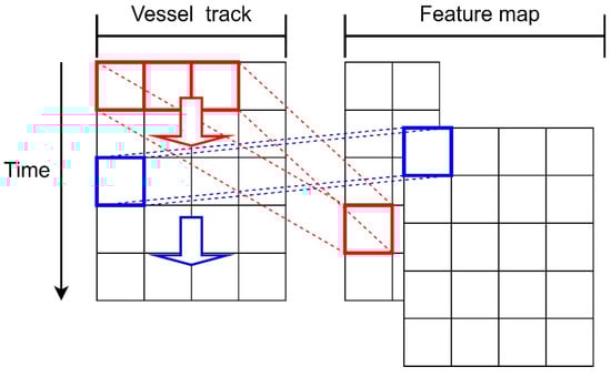
Figure 1.
Convolution kernel sliding over time. The red and blue convolutions represent two different window lengths of 1D CNN, and the feature maps are obtained by sliding over the vessel trajectory.
For this paper, the parallel multi-branch structure was used to fuse multi-scale features because it can acquire the features of different sensory fields at the same level of the data [26,27]. The multi-scale feature extraction and fusion of tracks is shown in Figure 2. The features are extracted by convolutional kernels of different sizes and are then passed to the next layer after concatenation in the dimension. Because relatively recent time steps have a great impact on the current time, we designed a one-dimensional convolution with window lengths of 1 (CNN-a) and 3 (CNN-b) to extract the features of the trajectory. Max-pooling was used after CNN to retain the main features while reducing parameters and preventing overfitting to improve the generalizability of the model.
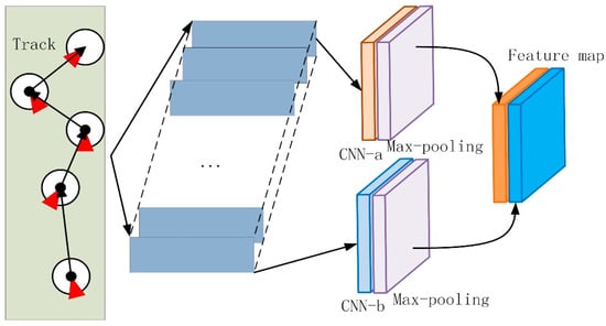
Figure 2.
Multi-scale feature extraction and fusion of tracks. The vessel tracks are pre-processed and input to the CNN with different window lengths to obtain the multi-scale feature map, and we subsequently fuse the feature maps in dimension.
In summary, multi-scale CNN extracts and concatenates specific features of multiple input data, which are subsequently fed into GRU for learning. We take advantage of the lightweight and fast computation of 1D CNN to obtain low-dimensional features, and we then use GRU for training, which is helpful for predicting long sequence information.
2.2. GRU Model
The gate structure of GRU can store and learn long sequence information that is suitable for trajectory prediction. In comparison with LSTM, the GRU model has one fewer gate function, and the prediction task can be accomplished with fewer model parameters, so we use GRU to forecast the trajectory in the complex environment of HF radar.
The internal structure of GRU is shown in Figure 3: is the sequence information input at time , is the hidden cell output at time , is the update gate, and is the reset gate.
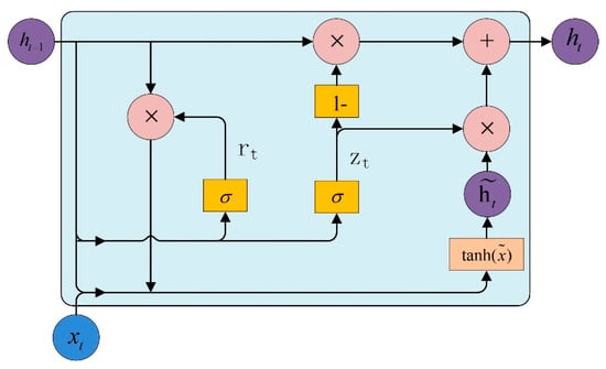
Figure 3.
Schematic diagram of the GRU neural network structure, which describes the detailed information of the transfer process.
The specific calculation process of GRU is as follows: First, the reset and update gates are generated by the sigmoid function from and the previous moment input . The reset gate determines how much state information from the previous moment should be retained. Second, the product of and is spliced with to obtain the hidden variable through the activation function. The update gate is the coefficient of the hidden variable. Larger coefficients indicate that more implicit variables are retained in the final output. Lastly, the linear combination of the historical information and the hidden variable contributes to the output of GRU unit . The GRU formula is as follows:
where , and are the weight matrix in the reset gate, the update gate, and the hidden variable, respectively, is the sigmoid function, and the function is a hyperbolic sine function. They are defined in Equations (6) and (7), respectively.
2.3. Attention Mechanism (AM)
In this paper, we use an AM to assign different weights to features in order to prevent the results from being disturbed by unimportant information and to improve the accuracy of the track prediction by helping the model filter useful information.
The AM is a weighted summation process [28]. In this paper, we use the temporal AM shown in Figure 4 to weight the characteristics learned by the stacked GRU. The algorithm distributes higher weights to features that have significant effects on the results, which is useful for improving the network’s forecasting.
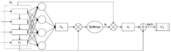
Figure 4.
Schematic diagram of the attention mechanism structure. The attention mechanism assigns different weights to the D-dimensional feature vectors.
First, the D-dimensional feature vectors () outputted by GRU are fully connected to obtain .
The feature of the last time step is multiplied by to get the value of score .
Then, after the function generates a weight corresponding to each feature. The larger the weight, the higher the relevance of the feature to the result.
The weights and the input features are multiplied to obtain the context vector .
Finally, and are merged in dimension, and the activation function is used to generate the weighted feature vector . is the fully connected layer weight after dimensional fusion.
2.4. AR Model
As a representative of linear prediction, the AR model has the advantages of simple structure and easy implementation by fitting the historical data to predict the future data. AR model is a linear regression model that employs a linear combination of random variables from several moments in the previous period to describe random variables at a later moment [29].
The AR model with random variable at time is based on a multiple linear regression of the previous moments . In this method, is considered to be primarily influenced by the serial values of past moments , and the error term is the random disturbance at that moment. The structure of the AR model is as follows:
The latitude and longitude information are sent to the network in parallel, and the AR model predicts them separately. The prediction of model is obtained by adding the outputs of the neural network part and the AR component.
2.5. Entropy Method
The entropy method belongs to a kind of objective assignment, which forms an objective and real evaluation system. This method uses information entropy, i.e., amount of information, to judge the weight of the index. The more information is provided by an indicator, the smaller the uncertainty and the corresponding information entropy.
The entropy weighting method works as follows. When our model uses the pre-break and post-break trajectories for forward and backward prediction, two results can be obtained. Then, we use the entropy weighting method to assign weights to both results by calculating the richness of information. The sum of the weights of the forward and backward estimation results in this article is 1, and the value of the weight reflects the importance of the two prediction results. The experiments in 3.4.1 show that the accuracy of the results after weighting is improved.
The entropy weighting method requires first normalizing the evaluation matrix to the range of . The information entropy of the -th indicator is then calculated as follows:
where is the -th sample value under the -th indicator.
In accordance with the information entropy, the weight of each indicator is calculated as follows:
2.6. Overall Model
In this paper, an HF radar-vessel broken-track prediction method based on MSCNN combined with GRU-AM and AR model is proposed, as shown in Figure 5. The trajectory was divided into a three-dimensional, structured time series, and the latitude and longitude information in the original HF radar data are processed in parallel. We used 1D CNNs with different window lengths to extract latitude and longitude features at different scales. The feature maps were concatenated in dimensions, and the features were fed into the stacked GRU. The stacked GRU model consisted of three layers of GRUs, and as the layers deepened, the GRU model became more capable of learning. The AM performs feature analysis on the input data and gives each feature a corresponding weight. Finally, the predicted track can be obtained from the fully connected layer. Because the AM can highlight information that has a significant impact on the results, the GRU model along with the AM can more fully mine effective information from the input data. In order to further improve the prediction accuracy of the algorithm, GRU-AM were then combined with the traditional AR linear model, and the two results are added to estimate the next time step of the trajectory, which improved the accuracy of track prediction.
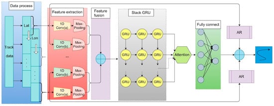
Figure 5.
Network structure of the proposed model.
We divided track into the pre-break track, the post-break track and the track at the break. We train the model using the pre-break track to get forward prediction, which is obtained by adding the prediction result of GRU-AM and the prediction result of AR. Similarly, we use the post-break track to obtain reverse prediction. The details are that the pre-break track was inputted into the model in the normal time step order, while the post-break track was inputted into the model in the opposite order, i.e., reversed. The reverse prediction results are again inverted to become the normal time order trajectories. The weights of the bidirectional prediction results are calculated by the entropy weight method, and we obtain the final predicted track by fusing the weighted sum of the two results. The process is shown in Figure 6.
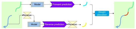
Figure 6.
Track fusion of the proposed model. The forward prediction is obtained by using the pre-break trajectory, the reverse prediction is obtained by using the post-break trajectory, and the final predicted trajectory is obtained by inverting the reverse prediction and weighting the two results by the entropy method.
3. Experiments and Analysis
In this section, we describe an experiments carried out on the basis of field HF radar data obtained from Huanghai, China on 20 July 2019. The parameters of the HF radar setting are as follows: carrier frequency 4.7M Hz, the number of array element 8. The signal-to-noise ratio of the radar is 9.47 dB, and the clutter-to-noise ratio is 6.86 dB.
As Figure 7 shows, the three traces have 1652, 1802, and 1002 time points, and the predicted intervals at the break are 36 min, 42 min, and 41 min, respectively. The longitude and latitude information and the relative positions of the three broken tracks can be seen on the HF radar detection map.
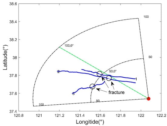
Figure 7.
Broken tracks of three vessels detected by HF radar. The red dot represents shore-based HF radar. The black corner sectors indicate the detection area of the HF radar. The blue lines indicate the moving trajectories of the three vessels, labeled 1, 2 and 3. The black oval is the mark of the fracture.
Section 3.1 describes the data processing before the experiment. Section 3.2 describes the parameter settings for the time steps and the number of iterations. Section 3.3 illustrates the specific parameters of the experimental network. Section 3.4 presents the prediction results, a comparison with other methods, and the ablation experiment. Section 3.5 illustrates how when the target in the RD spectrum is covered by sea clutter, the method in this paper can be used to make effective predictions.
3.1. Data Processing
The traces are processed into a three-dimensional time series structure that includes the number of points of a track , time step and feature dimension, which is suitable for GRU prediction. Longitude and latitude are each a single variable, so the shape of each input to the model is (, , 1).
To speed up the convergence of the model and improve its accuracy, the maximum-minimum normalization (min–max scaler) is used so that the values are all concentrated in the range . The formula is as follows:
where and represent the initial data and the normalised data, respectively.
In this paper, we adopt the sliding window method for data training, as shown in Figure 8. The sliding window is equivalent to a slider of a specified length sliding along the time series. The final data of the current slider can be predicted by sliding each unit until all the data in the training set have been traversed to complete an epoch of training.
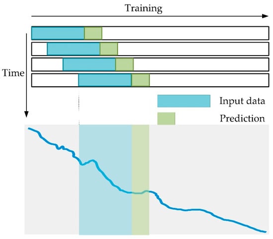
Figure 8.
Schematic diagram of track training over time, with blue representing the input training data and green representing the output corresponding to each batch of input. With the change of the training time, an epoch is finished when all the training sets are used.
3.2. Parameters Setting
The time step (tstep), i.e., the data from the first tstep moments used to forecast the data for the present moment, directly affects the accuracy of the estimation. To choose the appropriate value, the result errors are compared by setting different time steps (step = 3, 4, 5, 6, 7, 8, 9, 10). As Figure 9a shows, the error gradually decreases as the time step grows, while the error starts to rise after a time step of 8. The reason is that as the time step increases, more information can be used, leading to a more accurate prediction model. After the time step goes beyond a certain amount, however, the overly long series has less correlation with the current time, resulting in error accumulation and increase. The mean absolute error (MAE) and root mean square error (RMSE) are at a minimum when tstep = 8, so the time step is set at 8.
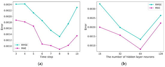
Figure 9.
(a) Error variation with time step. (b) Error variation with the number of hidden layer neurons. The blue line represents RMSE variation, and the purple line represents MAE variation.
To verify the effect of the number of neurons on the experiment, we set up a comparison experiment with the number of GRU neurons {16, 32, 64, 128}. The results are shown in Figure 9b, and we can see that the error decreases as the number of GRU neurons increases at the beginning. The error reaches the minimum when the number of GRU neurons is 64, but the error increases when the number of neurons increases further, so we set the number of neurons as 64.
Because the number of samples for each of the three traces is different, the early stopping method is used to find the most suitable number of iterations for each trace. The process consists of obtaining the test results of the verification set after the training of each epoch. As the training progresses, if the test error of the validation set decreases below a preset threshold, then the training is stopped and the current weights are saved as network parameters. This method can reduce overfitting, prevent overtraining, and reduce training time. We use the validation set loss (val-loss) as the data interface for monitoring, and set the threshold of loss reduction to 0 and the epoch of tolerance to 10; that is, the training is stopped when the loss is not reduced within 10 epochs. As Figure 10 shows, the loss of forward prediction for the three datasets converges at epoch = 120, 154, and 73, and the loss of the reverse estimation converges at epoch = 87, 128, and 68. The training ends when the loss converges, and the model parameters are saved immediately at that point.
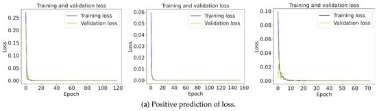
Figure 10.
Loss variation curve with the number of iterations. (a) represents forward training and (b) represents reverse training. The blue line is the training set and the yellow line is the validation set.
3.3. Implementation Details
All experiments were performed on a server equipped with a GTX1080Ti and 24 GB RAM. The software environment used was Python 3.7.6, Keras 2.1.4, and TensorFlow 1.14.
Our model embeds the input vector into 32 dimensions using the 1D CNN with kernel sizes of 1 and 3. The dimensions of the GRU hidden states are set to 64, and a total of 3 layers of GRUs are stacked. A sliding time window with a length of 8 and a stride size of 1 is used to get the training samples. The two fully connected layers have hidden state dimensions of 64 and 2. The network model weights are updated using the Adam optimizer, with MSE as the loss function. The batch size is 32 and the learning rate is 0.001.
After training, the test data are fed into the model for prediction and the results are inverse normalized to change them into the original order of magnitude. This process is shown in Figure 11.
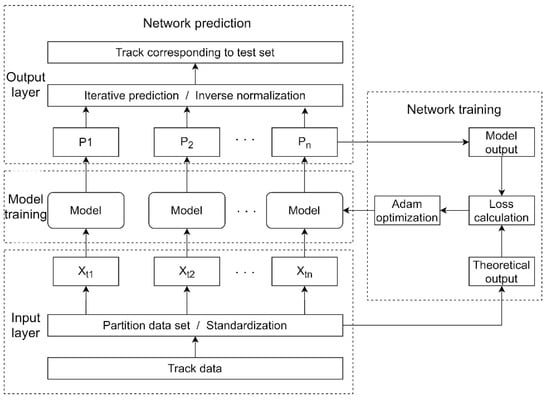
Figure 11.
Training process of the proposed network. The original ship trajectory data are input to the prediction model after data segmentation and normalization. The model is trained through iterations to output the prediction results, and the results are back-normalized to obtain the predicted trajectories.
The root mean square error (RMSE) and mean absolute error (MAE) are used to test the degree of deviation of the model-forecast trajectory from the correct value, and we use () as the unit of measurement. They are defined by Equations (17) and (18):
where is the number of fracture points of a track, i.e., points of coordinates, and indicate the predicted and true values, respectively.
3.4. Experiment Results Analysis
3.4.1. Experiment Results
We use the pre-break track information to obtain forward prediction track, and the post-break track information to obtain reverse prediction track. The entropy method calculates the corresponding weights of the two forecast results by analyzing the trajectories predicted by the data before and after the fracture. The weighting parameters assigned by the entropy method are shown in Table 1.

Table 1.
Weighting parameters assigned by the entropy method.
The forward and reverse predicted results are added by the assigned weights to get the final trajectory. Table 2 shows the error of the forward prediction track, the error of the reverse prediction track, and the error of the final track obtained by the weighted fusion of the two, respectively. It can be seen that the fused track errors are further reduced.
Table 2.
Changes in indicators before and after fusion.
The data before and after the break in the three traces are used as training samples for prediction, and the results are weighted and fused into new traces. The final trace result figures are shown in Figure 12. It can be seen that the method proposed in this paper can effectively predict HF radar-vessel broken tracks.
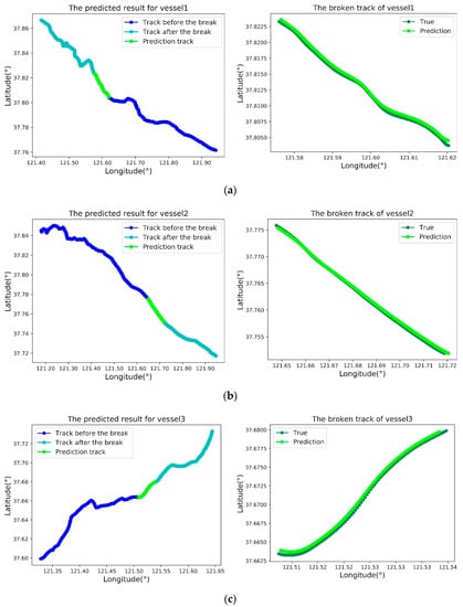
Figure 12.
(a–c) represent the 3 broken tracks, respectively. The diagrams on the left show the predicted results of the three fractured trajectories. The blue, cyan, and green lines represent, respectively, the trace before the break, the trace after the break, and the predicted track at the fracture. The graphs on the right show the comparison between the predicted and real values at the fracture.
3.4.2. Comparison Experiments
The performance of the proposed method is compared with four deep learning methods: sequence to sequence (Seq2Seq), LSTM, bidirectional LSTM (Bi-LSTM), and a statistical filtering algorithm: the extended Kalman filter (EKF). To ensure the fairness of the experiment, the parameters of the four methods are kept as consistent as possible. Figure 13 shows the prediction results of the proposed method and the other four methods. It can be observed that the method in this article is closest to the actual track.
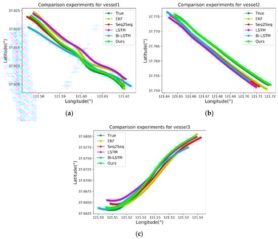
Figure 13.
The effect of the compared methods is shown. The prediction results of the proposed method and other mainstream algorithms including EKF, Seq2Seq, LSTM and Bi-LSTM for the three trajectories are shown in (a–c), respectively.
- EKF: The system noise variance matrix and the observation noise variance , where is a diagonal matrix.
- Seq2Seq: The encoder has three layers of GRU, and the decoder has one layer of GRU. Each GRU layer has 128 neurons.
- LSTM: Three stacked layers are used in LSTM with 128 neurons in each layer, and is used as the activation function.
- Bi-LSTM: Three stacked layers are used in LSTM with 64 neurons in each layer.
In addition to the regression metrics RMSE and MAE as the evaluation criteria, we added the mean range error (MRE) to provide a more intuitive understanding of the prediction effect of each method. MRE uses Haversine formula to convert two corresponding latitude and longitude coordinates and into the actual distance between the two points. Finally, the average distance in km of this track is calculated. The formula is as follows:
where , 6371 km and is the number of fracture points of a track, i.e., points of coordinates.
Taking the regression indicators RMSE, MAE and MRE as evaluation criteria, it can be seen from Table 3 that the prediction performance of the new method is better than those of the other four methods.
Table 3.
Comparison of the proposed method with other four baseline methods for different tracks.
3.4.3. Ablation Experiments
To verify the effectiveness of the proposed method, the AR model, the AM, and the MSCNN are removed and named no-ar, no-am, and no-mscnn, respectively. The results of the ablation experiments are shown in Figure 14. The following conclusions can be drawn:
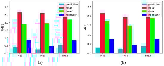
Figure 14.
Ablation experiments with RMSE in (a) and MAE in (b). The values of line 1 and line 3 are 10−3, and line 2 is 10−2.
- The complete model has the least RMSE and MAE, indicating that all components contribute to the effectiveness and robustness of the overall model.
- The performance of the model without AR and AM drops significantly, indicating that the AR and AM models play a crucial role. The main reason is that the AM model can enhance the results, and the AR network can effectively predict the linear information in the trajectory. In addition, it was found that the network performance decreases the most after the AR model is removed, showing that this model has a significant impact on the results. The reason is that the time series signal can be modeled by AR [30] and AR is generally robust to the scale changing of the data [31].
- There is also a performance loss when multiscale convolution is removed from the model, but the loss is less than when the AM and AR models are removed. This is due to the strong learning ability of stacked GRUs, together with the screening ability of attention and the joint effect of AR. Even if the multi-scale convolution module is removed, causing a performance loss, some of the missing features can still be obtained by other components of the model.
3.5. Comparison with RD Spectrum
This section illustrates the prediction performance using the method of this paper when the vessel is concealed in clutter with an RD spectrum. The RD spectrum can show the distance and speed of the marine target detected by HF radar and the distribution of the clutter. The AIS data can provide specific position information for the ship, so the AIS data superimposed on the RD spectrum can obtain the vessel’s orientation data and the real time of the ship’s entering and leaving the clutter [32,33]. When the vessel target is submerged in sea clutter and produces a broken track, it is difficult to identify the vessel in the RD spectrum obtained by HF radar. For this reason, we used the data from before and after the break to predict the trajectory at the sea clutter in both directions, and then obtained the vessel’s trajectory within the clutter.
Figure 15 shows the whole process of a target vessel, ship number 413134000 (framed by a black square), encountering sea clutter while passing an area in the Yellow Sea on 20 July 2019. It can be seen that the vessel entered the sea clutter at the moment in Figure 15a and started to be covered by the sea clutter. At that time, the vessel could not be accurately detected by HF radar alone. At the moment, in Figure 15b, the vessel was completely covered in the clutter region. The vessel left the sea clutter area at the moment in Figure 15c and was detected by HF radar again. The whole disappearance process passed through 11 batches, i.e., 11 min.
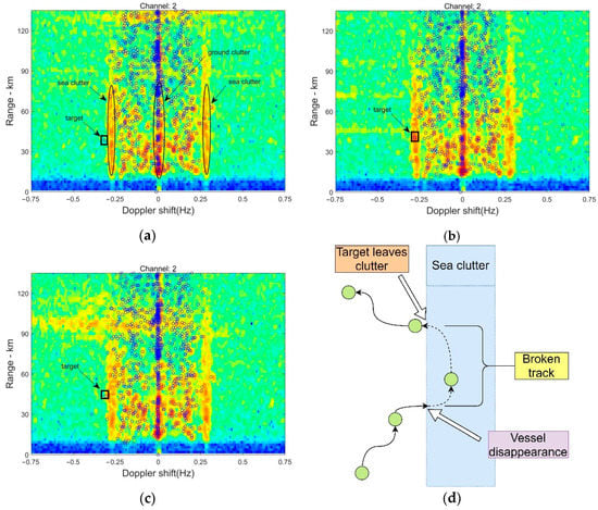
Figure 15.
The black ellipses are clutter (sea clutter on both sides and ground clutter in the middle), the blue circles are the vessels detected by AIS, and the black box is the target vessel. (a) The target vessel is sailing toward the sea clutter zone. (b) The target vessel is covered by the clutter region. (c) The target vessel is leaving the sea clutter zone. (d). Schematic diagram of the target vessel entering and leaving the sea clutter.
Our model can effectively resolve the difficulties of vessel tracking under strong clutter. The comparative experimental index is shown in Table 4.
Table 4.
Comparison of the proposed method with the other four baseline methods in terms of RMSE, MAE and MRE.
As Figure 16 shows, by forecasting the trajectory during the time of the vessel’s disappearance and comparing the prediction result with the real AIS data, it can be seen that even if the target disappears temporarily, its location can be accurately estimated using the method proposed in this paper.
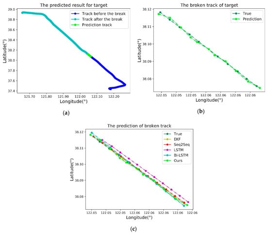
Figure 16.
(a) The real target trajectory verification. The blue, cyan, and green lines represent, respectively, the track before the break, the track after the break, and the predicted track at the break. (b) Comparison of the forecast and the real AIS data. (c) Comparison of the broken track prediction with the other mainstream algorithms including EKF, Seq2Seq, LSTM and Bi-LSTM.
4. Discussion
To investigate whether the method is effective in the case of substantial course and speed maneuvers, we select real track data with strong course maneuvers and speed maneuvers for experiments.
4.1. Course Maneuvers
We select the course maneuver in the vessel 1 trajectory and set the break in the course maneuvers at 7 min. Figure 17 shows that the points near the beginning and end of the turn are predicted more accurately, while several points in the middle of the turn are slightly off. Because this paper uses the trajectory before and after the break to predict the break in both directions, the start and end points of the blue line segment are at the beginning of the forward and the reverse predictions. For this reason, the prediction is more accurate. With the increase in accumulated errors, the prediction points in the middle section of the trajectory deviate slightly, but the overall course maneuvers are well predicted, with RMSE = 0.002256, MSE = 0.001790 and MRE = 0.165710.

Figure 17.
The part of the trajectory broken during the course maneuvers. The blue and brown lines show the real and predicted tracks, respectively. The box in the lower left compares the real and predicted tracks at the point where the break occurred.
4.2. Speed Maneuvers
We select the speed maneuver in the vessel 3 trajectory and set the break in the speed maneuvers at 8 min. In Figure 18, the blue line segment shows that the ship is performing an accelerated motion, and the proposed method in this paper can make a good prediction of the speed maneuver, with RMSE = 0.001686, MAE = 0.001484 and MRE = 0.131175.
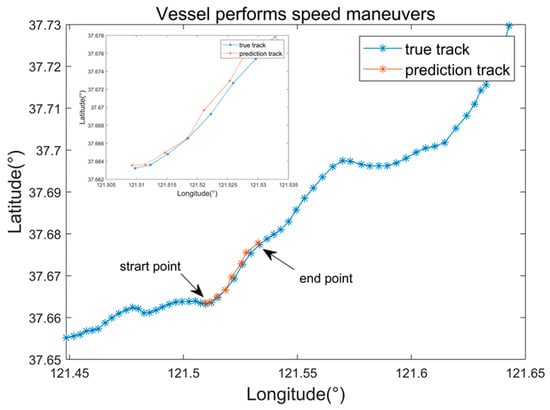
Figure 18.
The track breaking during a speed maneuver. The blue and brown lines show the real and predicted tracks, respectively. The figure in the upper left compares the real and predicted tracks at the point where the break occurred during the maneuver.
5. Conclusions
To overcome the difficulties of tracking targets concealed in strong clutter or interference, we propose a method based on MSCNN, combing GRU-AM and fusion with the AR model to solve the problem of broken track prediction with HF radar vessels. According to the findings in this paper, diverse features are extracted more effectively by MSCNN than by other methods. The features are sent into the stacked GRU, which can retain effective memory information as much as possible and solve the gradient dispersion problem. By using the temporal AM to calculate the weights of different features, we can give more attention to important features. Additionally, by integrating the AR model with nonlinear neural networks in parallel, we achieve univariate time series and multivariate time series predictions, and the combination of linear and nonlinear models.
Unlike traditional one-way track-estimation methods, we use the pre-break trajectory for forward estimation and the post-break trajectory for backward forecasting. This not only fully utilizes the available data, it also demonstrates that fusing the bidirectional prediction results can further improve the estimation accuracy. The field experiments show that the new method in this paper outperforms the other mainstream methods in terms of RMSE, MAE and MRE index evaluation, so our method is suitable for HF radar vessel broken-track prediction in complex environments with strong clutter and interference. In addition, the prediction results are validated by AIS data, which show the effectiveness of our method in estimating the broken tracks of HF radar targets concealed in clutter.
Furthermore, simulation experiments on the vessel performing course and speed maneuvers were conducted to verify the effectiveness of our method. In our future work, if more trajectory sample data concealed in clutters can be obtained, a deeper network model for multi-scale feature extraction such as ResNet can be designed. This scheme can be applied to HF radar target tracking in more complex environments with strong sea clutter, ionospheric clutter, and radio frequency interference.
Author Contributions
Conceptualization: L.Z.; Methodology: J.Z. and G.L.; Software: J.Z. and G.L.; Validation: J.Z. and J.N.; Investigation: J.Z.; Resources: J.N.; Data curation: L.Z.; Writing—original draft preparation: L.Z. and J.Z.; Project administration: L.Z.; Writing—review and editing: Q.M.J.W.; J.Z. and L.Z. are co-first authors and contribute equally to this work. All authors have read and agreed to the published version of the manuscript.
Funding
This project is sponsored by National Key R&D Program of China (No. 2017YFC1405202), and the National Natural Science Foundation of China (No. 51979256).
Institutional Review Board Statement
Not applicable.
Informed Consent Statement
Not applicable.
Data Availability Statement
The data presented in this study are available on request from the corresponding author. The data are not publicly available due to privacy restrictions.
Conflicts of Interest
The authors declare no conflict of interest. The funders had no role in the design of the study; the collection, analyses, or interpretation of the data; the writing of the manuscript; or the decision to publish the results.
References
- Ponsford, A.M.; Wang, J. A review of High Frequency Surface Wave Radar for detection and tracking of ships. Turk. J. Electr. Eng. Comput. Sci. 2010, 18, 409–428. [Google Scholar] [CrossRef]
- Sun, W.; Ji, M.; Huang, W.; Ji, Y.; Dai, Y. Vessel tracking using bistatic compact HFSWR. Remote Sens. 2020, 12, 1266. [Google Scholar] [CrossRef]
- Zhang, L.; Mao, D.; Niu, J.; Jonathan Wu, Q.M.; Ji, Y. Continuous tracking of targets for stereoscopic HFSWR based on IMM filtering combined with ELM. Remote Sens. 2020, 12, 272. [Google Scholar] [CrossRef]
- Rigatos, G.G. Sensor fusion-based dynamic positioning of ships using Extended Kalman and Particle Filtering. Robotica 2013, 31, 389–403. [Google Scholar] [CrossRef]
- Perera, L.P.; Oliveira, P.; Soares, C.G. Maritime traffic monitoring based on vessel detection, tracking, state estimation, and trajectory prediction. IEEE Trans. Intell. Transp. Syst. 2012, 13, 1188–1200. [Google Scholar] [CrossRef]
- Vivone, G.; Braca, P.; Horstmann, J. Knowledge-Based Multitarget Ship Tracking for HF Surface Wave Radar Systems. IEEE Trans. Geosci. Remote Sens. 2015, 53, 3931–3949. [Google Scholar] [CrossRef]
- Osborne, R.W.; Blair, W.D. Update to the hybrid conditional averaging performance prediction of the IMM algorithm. IEEE Trans. Aerosp. Electron. Syst. 2011, 47, 2967–2974. [Google Scholar] [CrossRef]
- Zhou, H.; Chen, Y.; Zhang, S. Ship Trajectory Prediction Based on BP Neural Network. J. Artif. Intell. 2019, 1, 29–36. [Google Scholar] [CrossRef]
- Liu, J.; Shi, G.; Zhu, K. Vessel trajectory prediction model based on ais sensor data and adaptive chaos differential evolution support vector regression (ACDE-SVR). Appl. Sci. 2019, 9, 2983. [Google Scholar] [CrossRef]
- De Masi, G.; Gaggiotti, F.; Bruschi, R.; Venturi, M. Ship motion prediction by radial basis neural networks. In Proceedings of the 2011 IEEE Workshop On Hybrid Intelligent Models And Applications, Paris, France, 11–15 April 2011; pp. 28–32. [Google Scholar] [CrossRef]
- Pascanu, R.; Mikolov, T.; Bengio, Y. On the difficulty of training recurrent neural networks. In Proceedings of the 30th International Conference on Machine Learning. ICML 2013, Atlanta, GA, USA, 16–21 June 2013; pp. 2347–2355. [Google Scholar]
- Hochreiter, S.; Schmidhuber, J. Long Short-Term Memory. Neural Comput. 1997, 9, 1735–1780. [Google Scholar] [CrossRef]
- Cho, K.; Van Merriënboer, B.; Gulcehre, C.; Bahdanau, D.; Bougares, F.; Schwenk, H.; Bengio, Y. Learning phrase representations using RNN encoder-decoder for statistical machine translation. In Proceedings of the EMNLP 2014—2014 Conference on Empirical Methods in Nature Language Processing Proceeding of the Conference, Doha, Qatar, 25–29 October 2014; pp. 1724–1734. [Google Scholar] [CrossRef]
- Yang, S.; Yu, X.; Zhou, Y. LSTM and GRU Neural Network Performance Comparison Study: Taking Yelp Review Dataset as an Example. In Proceedings of the 2020 International Workshop on Electronic Communication and Artificial Intelligence. IWECAI 2020, Qing Dao, China, 12–14 June 2020; pp. 98–101. [Google Scholar] [CrossRef]
- del Águila Ferrandis, J.; Triantafyllou, M.; Chryssostomidis, C.; Karniadakis, G. Learning functionals via LSTM neural networks for predicting vessel dynamics in extreme sea states. arXiv 2019, arXiv:1912.13382. [Google Scholar] [CrossRef]
- Yuan, Z.; Liu, J.; Liu, Y.; Zhang, Q.; Liu, R.W. A multi-task analysis and modelling paradigm using LSTM for multi-source monitoring data of inland vessels. Ocean Eng. 2020, 213, 107604. [Google Scholar] [CrossRef]
- Gao, M.; Shi, G.; Li, S. Online prediction of ship behavior with automatic identification system sensor data using bidirectional long short-term memory recurrent neural network. Sensors (Switzerland) 2018, 18, 4211. [Google Scholar] [CrossRef] [PubMed]
- Zhang, G.; Tan, F.; Wu, Y. Ship Motion Attitude Prediction Based on an Adaptive Dynamic Particle Swarm Optimization Algorithm and Bidirectional LSTM Neural Network. IEEE Access 2020, 8, 90087–90098. [Google Scholar] [CrossRef]
- Agarap, A.F.M. A neural network architecture combining gated recurrent unit (GRU) and support vector machine (SVM) for intrusion detection in network traffic data. ACM Int. Conf. Proceeding Ser. 2018, 26–30. [Google Scholar] [CrossRef]
- Suo, Y.; Chen, W.; Claramunt, C.; Yang, S. A ship trajectory prediction framework based on a recurrent neural network. Sensors (Switzerland) 2020, 20, 5133. [Google Scholar] [CrossRef]
- Forti, N.; Millefiori, L.M.; Braca, P.; Willett, P. Prediction oof Vessel Trajectories from AIS Data Via Sequence-To-Sequence Recurrent Neural Networks. In Proceedings of the 2020 IEEE International Conference on Acoustics, Speech and Signal Processing (ICASSP), Barcelona, Spain, 4–8 May 2020; pp. 8936–8940. [Google Scholar] [CrossRef]
- Luong, M.T.; Pham, H.; Manning, C.D. Effective approaches to attention-based neural machine translation. In Proceedings of the Conference Proceedings-EMNLP 2015: Conference Empirical Methods in Nature Language Processing, Lisbon, Portugal, 17–21 September 2015; pp. 1412–1421. [Google Scholar] [CrossRef]
- Cheng, X.; Li, G.; Ellefsen, A.L.; Chen, S.; Hildre, H.P.; Zhang, H. A Novel Densely Connected Convolutional Neural Network for Sea-State Estimation Using Ship Motion Data. IEEE Trans. Instrum. Meas. 2020, 69, 5984–5993. [Google Scholar] [CrossRef]
- Raghu, J.; Srihari, P.; Tharmarasa, R.; Kirubarajan, T. Comprehensive Track Segment Association for Improved Track Continuity. IEEE Trans. Aerosp. Electron. Syst. 2018, 54, 2463–2480. [Google Scholar] [CrossRef]
- Meliboev, A.; Alikhanov, J.; Kim, W. 1D CNN based network intrusion detection with normalization on imbalanced data. arXiv 2020, arXiv:2003.00476. [Google Scholar]
- Szegedy, C.; Liu, W.; Jia, Y.; Sermanet, P.; Reed, S.; Anguelov, D.; Erhan, D.; Vanhoucke, V.; Rabinovich, A. Going deeper with convolutions. In Proceedings of the IEEE Computer Society Conference Computer Vision and Pattern Recognition, Boston, MA, USA, 7–12 June 2015; pp. 1–9. [Google Scholar] [CrossRef]
- Shelhamer, E.; Long, J.; Darrell, T. Fully Convolutional Networks for Semantic Segmentation. IEEE Trans. Pattern Anal. Mach. Intell. 2017, 39, 640–651. [Google Scholar] [CrossRef]
- Abedinia, O.; Amjady, N.; Zareipour, H. A New Feature Selection Technique for Load and Price Forecast of Electrical Power Systems. IEEE Trans. Power Syst. 2017, 32, 62–74. [Google Scholar] [CrossRef]
- Javeri, I.Y.; Toutiaee, M.; Arpinar, I.B.; Miller, T.W.; Miller, J.A. Improving Neural Networks for Time Series Forecasting using Data Augmentation and AutoML. arXiv 2021, arXiv:2103.01992. [Google Scholar]
- Moon, J.; Hossain, M.B.; Chon, K.H. AR and ARMA model order selection for time-series modeling with ImageNet classification. Signal Processing 2021, 183, 108026. [Google Scholar] [CrossRef]
- Lai, G.; Chang, W.C.; Yang, Y.; Liu, H. Modeling long- and short-term temporal patterns with deep neural networks. In Proceedings of the 41st International ACM SIGIR Conference Research and Development in Information Retrieval, SIGIR 2018, Ann Arbor, MI, USA, 8–12 July 2018; pp. 95–104. [Google Scholar] [CrossRef]
- Yang, K.; Zhang, L.; Niu, J.; Ji, Y.; Jonathan Wu, Q.M. Analysis and Estimation of Shipborne HFSWR Target Parameters Under the Influence of Platform Motion. IEEE Trans. Geosci. Remote Sens. 2020, 1–14. [Google Scholar] [CrossRef]
- Redoutey, M.; Scotti, E.; Jensen, C.; Ray, C.; Claramunt, C. Efficient vessel tracking with accuracy guarantees. In Proceedings of the International Symposium on Web and Wireless Geographical Information Systems, Shanghai, China, 11–12 December 2008; 2008; pp. 140–151. [Google Scholar] [CrossRef]
Publisher’s Note: MDPI stays neutral with regard to jurisdictional claims in published maps and institutional affiliations. |
© 2021 by the authors. Licensee MDPI, Basel, Switzerland. This article is an open access article distributed under the terms and conditions of the Creative Commons Attribution (CC BY) license (https://creativecommons.org/licenses/by/4.0/).