Article

An Optimal Image–Selection Algorithm for Large-Scale Stereoscopic Mapping of UAV Images

1
Image Engineering Research Center, 3DLabs Co. Ltd., Incheon 21984, Korea
2
Department of Geoinformatic Engineering, Inha University, Incheon 22212, Korea
3
Center of RS & GIS, Korea Polar Research Institute, Incheon 21990, Korea
4
Department of Civil Engineering, Gyeongsangnam National University of Science and Technology, Jinju 52725, Korea
*
Author to whom correspondence should be addressed.
Remote Sens. 2021, 13(11), 2118; https://doi.org/10.3390/rs13112118
Submission received: 31 March 2021 / Revised: 17 May 2021 / Accepted: 20 May 2021 / Published: 28 May 2021
(This article belongs to the Special Issue UAV Photogrammetry and Remote Sensing)

Abstract

:
Recently, the mapping industry has been focusing on the possibility of large-scale mapping from unmanned aerial vehicles (UAVs) owing to advantages such as easy operation and cost reduction. In order to produce large-scale maps from UAV images, it is important to obtain precise orientation parameters as well as analyzing the sharpness of they themselves measured through image analysis. For this, various techniques have been developed and are included in most of the commercial UAV image processing software. For mapping, it is equally important to select images that can cover a region of interest (ROI) with the fewest possible images. Otherwise, to map the ROI, one may have to handle too many images, and commercial software does not provide information needed to select images, nor does it explicitly explain how to select images for mapping. For these reasons, stereo mapping of UAV images in particular is time consuming and costly. In order to solve these problems, this study proposes a method to select images intelligently. We can select a minimum number of image pairs to cover the ROI with the fewest possible images. We can also select optimal image pairs to cover the ROI with the most accurate stereo pairs. We group images by strips and generate the initial image pairs. We then apply an intelligent scheme to iteratively select optimal image pairs from the start to the end of an image strip. According to the results of the experiment, the number of images selected is greatly reduced by applying the proposed optimal image–composition algorithm. The selected image pairs produce a dense 3D point cloud over the ROI without any holes. For stereoscopic plotting, the selected image pairs were map the ROI successfully on a digital photogrammetric workstation (DPW) and a digital map covering the ROI is generated. The proposed method should contribute to time and cost reductions in UAV mapping.

1. Introduction

Unmanned aerial vehicles (UAVs) were initially developed for military uses, such as reconnaissance and surveillance. Their utilization has been expanded to industrial and civilian purposes, such as precision agriculture, change detection and facility management. UAVs are equipped with various sensors, such as optical and infrared sensors. Optical sensors installed in UAVs are small non-metric digital cameras due to their limited weight and power. UAVs usually capture images at higher resolutions than manned aerial vehicles due to their low flight altitudes. They also acquire images rapidly. Due to these advantages, the mapping industry has developed a great interest in large-scale map production using UAVs [1,2,3].
For large-scale mapping, it is important to have precise orientation parameters (OPs) for UAV images. OPs can be classified into interior orientation parameters (IOPs) and exterior orientation parameters (EOPs). IOPs are related to imaging sensors mounted on UAVs, such as focal length and lens distortion. They can be estimated through camera calibration processes [4,5,6]. EOPs are related to the pose of the UAVs during image acquisition, such as position and orientation. Initial EOPs are provided by navigation sensors installed in the UAV. They are refined through bundle adjustment processes [7,8]. These techniques are also included in most commercial UAV image processing software.
For large-scale mapping, it is important to select optimal images to be used. UAVs need a large number of images to cover a region of interest (ROI), often with a high overlap ratio. One needs to cover the ROI with the fewest possible images. Otherwise, to map the ROI, one may have to handle too many UAV images. For this reason, stereo plotting of UAV images in particular is time consuming and costly.
Previous research on large-scale mapping using UAVs dealt with mapping accuracy analysis [9], accuracy in 3D model extraction [10,11,12] and image mosaicking [13,14,15,16]. On the other hand, studies on reducing the number of images for mapping or stereoscopic plotting were difficult to find. We believe there is a strong need for research on how to select optimal UAV images for stereoscopic mapping in particular.
This study proposes an intelligent algorithm to select a minimum number of image pairs that can cover the ROI, or to select a minimum number of the most accurate image pairs to cover the ROI. UAV images are grouped into strips and the initial image pairs are formed from among images within the same strip. We then apply an intelligent scheme to iteratively select the optimal image pairs from the start to the end of an image strip. Through the proposed image selection method, the ROI can be covered by either the minimum number of image pairs or the most accurate image pairs. The selected image pairs produce a dense 3D point cloud over the ROI without any holes. For stereoscopic plotting, the selected image pairs successfully mapped the ROI on a digital photogrammetric workstation (DPW), and a digital map covering the ROI was generated.

2. Proposed Method

The steps of the proposed algorithm are shown in Figure 1. Images are first grouped into strips. In this paper, we assume that images with bundle adjustment are taken in multiple linear strips. We need this process to confine pair selection and stereoscopic mapping to images within the same strip. Secondly, overlaps among images within the same strip are calculated. Any two images with overlapping regions are defined as initial image pairs. For initial pair composition, one may impose geometric constraints such minimum overlap ratio or Y-parallax limits. The Y-parallax is a vertical coordinate difference between left and right tie points mapped from an origin image to an epipolar image through epipolar resampling. The closer the Y-parallax is to zero, the higher the accuracy [17]. Next, optimal image pairs are determined by an iterative pair-selection process. Among images paired with the first image within a strip, a first optimal pair is selected by using prioritized geometric constraints. Images paired with subsequent images within the strip are checked against the pair selected first. All image pairs overlapping the selected pair are candidates for the next optimal pair. We select the next pair according to specific criteria. All other pairs are considered redundant and are removed from further processing. Selection is repeated with the new optimal pair until reaching the end of the image strip.

2.1. Image Grouping into Strips

For optimal image-pair selection, images are first grouped into strips. In this paper, we develop a scheme for image grouping based on linear strips. This scheme needs to be adapted to other types, such as circular strips.
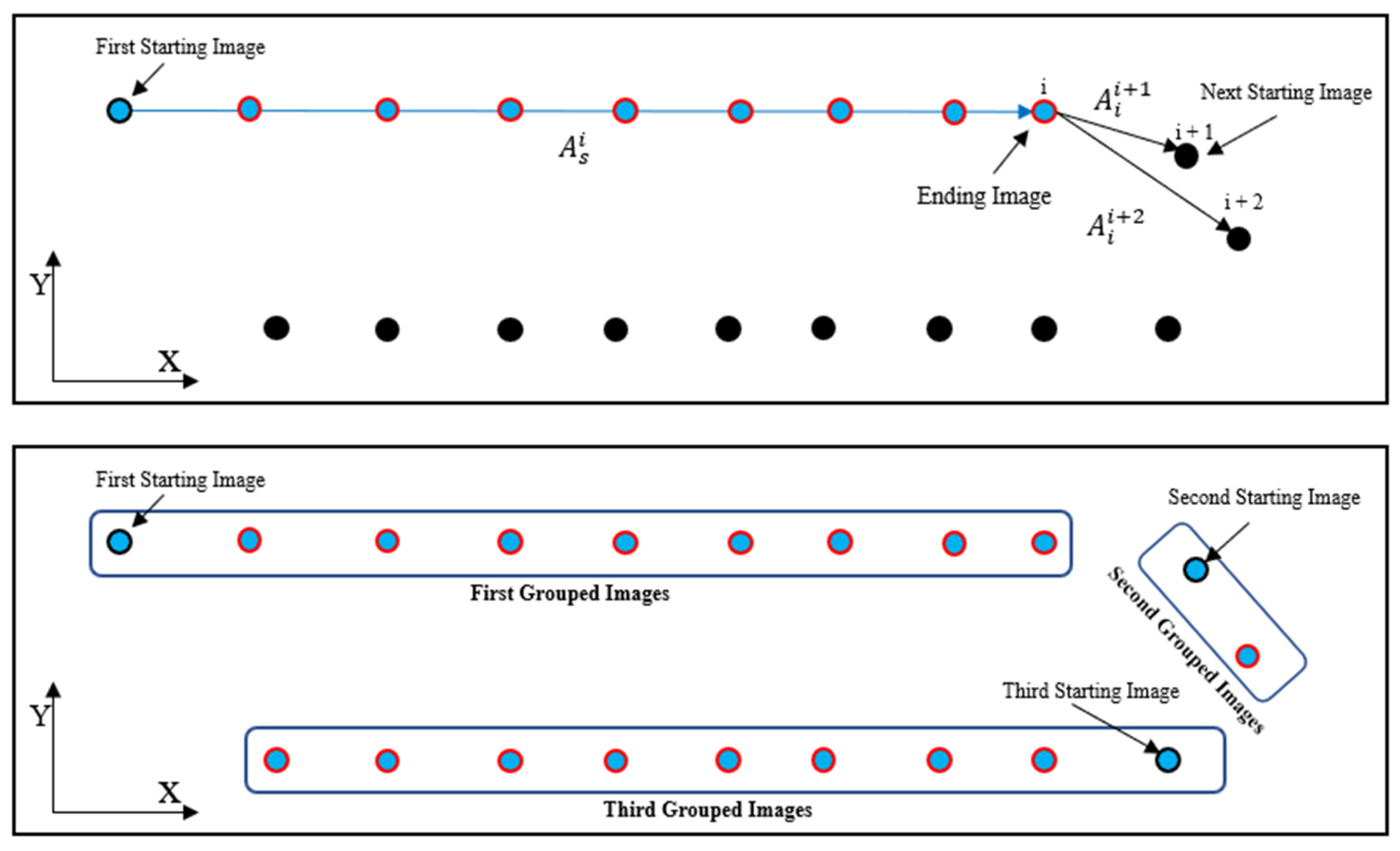
Images are grouped into strips by comparing the EOPs among successive images in a sequence. Figure 2 shows an example of image grouping and its result. The first image within a sequence is defined as a starting image. An image strip is formed by the first and second images of the sequence. Next, azimuth A s i is calculated between the starting image and the i-th image, which is the last image of the strip. Similarly, the azimuth between the i-th image and image i + 1 ( A i i + 1 ) is calculated. The formulas for A s i and A i i + 1 are
A s i = tan 1 ( Y i Y s X i X s )
A i i + 1 = tan 1 ( Y i + 1 Y i X i + 1 X i )
In the above equations,   X s and   Y s are the coordinates of the starting image, X i   and   Y i are coordinates for the i-th image and X i + 1   and   Y i + 1 are for image i + 1. If the difference between A s i and A i i + 1 is less than a set threshold, we include image i + 1 in the same group as the starting image. In this case, the image-grouping process continues with the starting image, image i + 1 and image i + 2. When the angle difference is more than the threshold, we check the angle between the i-th image and image i + 2 ( A s i + 2 ). This is to avoid undesirable effects from accidental drift by the UAV. If the difference between A s i and A i i + 2 is also more than the threshold, the i-th image is defined as the final image of the current image group. In this case, image i + 1 is defined as a new image of a new image group. The image grouping process restarts with the new starting image.
After the image grouping process is completed for the entire image sequence, image groups with a small number of images are assumed to be outside the ROI and can be removed from further processing. The bottom image in Figure 2 shows the grouping result. In this example, the second group will be removed.

2.2. Initial Image Pair Composition

Once images are grouped into strips, overlaps between adjacent images within the same strip are estimated. First, the ground coverage of individual images is calculated by projecting image corner points onto the ground reference plane though the collinear equations in (3) and (4) below.
[ X P X O Y P Y O Z P Z O ] = λ   [ r 11 r 12 r 13 r 21 r 22 r 23 r 31 r 32 r 33 ] [ x p y p f ]
In the collinear equations, Xp, Yp and Zp are the object coordinates of point P on the ground, while XO, YO and ZO denote the position of the camera projection center; λ is a scale constant; xp and yp are the coordinates of p in the image, f is the focal length and r11 to r33 are rotation matrix parameters calculated from orientation angles. Zp is the approximated height of the ground reference plane. It can be calculated by the average height of ground control points (GCPs), if any, or by the average height of tie points.
X P = r 11 x p + r 12 y p r 13 f r 31 x p + r 32 y p r 33 f ( Z P Z o ) + X o
Y P = r 21 x p + r 22 y p r 23 f r 31 x p + r 32 y p r 33 f ( Z P Z o ) + Y o
Z P =   Height   of   Ground   Reference   Plane
Once individual image coverages are calculated, an overlapping area between two images is calculated based on the ground reference plane (Figure 3) [18,19,20]. As shown in Figure 3, the coverage of the reference image and that of the target image define the reference polygon and target polygon, respectively. Vertices of overlap polygon are defined by the corner points of corresponding images and the intersection of the reference polygon and target polygon. Once the overlap included in the vertices is calculated, the polygon is defined atop the overlap for further processing.
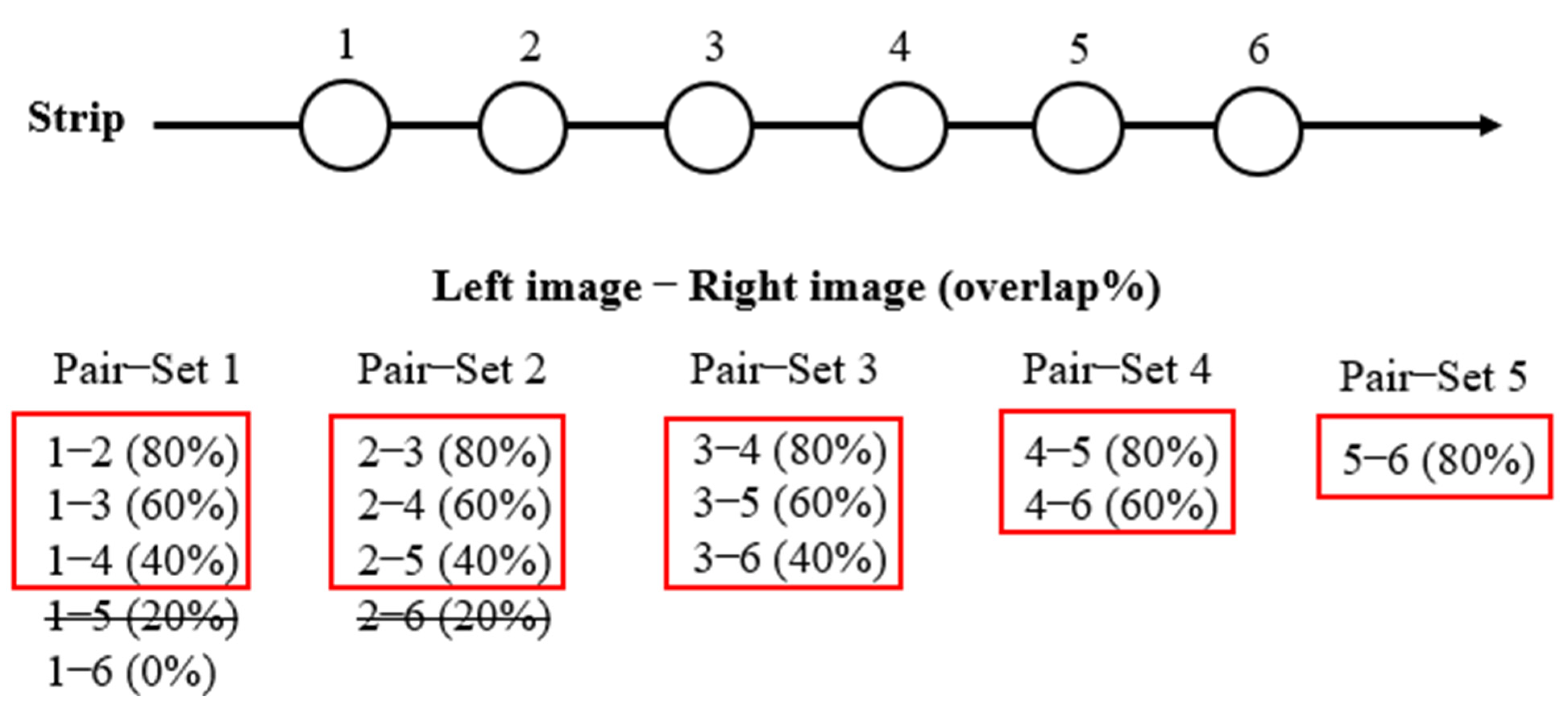
If there is any overlap between two images, the two images are defined as an initial image pair. In this process, one may apply a minimum overlap ratio (20%, for example) as a limit for initial image-pair selection. One may also impose stereoscopic quality measures for initial image-pair selection. Y-parallax errors among image pairs are good candidates for measurement [11,18,19], and can help explain how well two images will align after epipolar rectification. Convergence angles are also good candidates. When they are too small or too large, two images are likely to form weak stereo geometry and bring accuracy degradation [20,21]. Additional parameters, such as asymmetric and bisector elevation angles [20,21], can be considered, although they may not be dominant factors for stereoscopic quality in UAV images.
Figure 4 shows an example of initial image pairs in a strip with six images. The ground coverage of the first image (1) is checked with that of subsequent images. Image 1 overlaps images 2, 3 and 4. It does not overlap 5 or 6 at a ratio of more than 20%. An image-pair set for image 1 (Pair-Set 1) is defined comprising image pairs 1–2, 1–3 and 1–4. Similarly, image-pair sets are defined for images 2, 3, 4 and 5. There are 12 image pairs in total for the image strip. A simple selection of image pairs from among the 12 defined pairs could be done by choosing one image pair per Pair-Set. For example, one can select pairs with neighboring images within the image sequence, and five image pairs will be selected. However, this selection may contain redundancies, and may not offer the best accuracy. We need a more intelligent strategy for pair selection.

2.3. Optimal Pair Selection

From the initial image pairs, optimal image pairs can be selected to cover the ROI according to the desired selection criterion. In this paper, we describe two such criteria: minimum pair selection and most accurate pair selection. One may apply other criteria according to individual requirements.
The process starts by selecting a reference pair from among image pairs in the Pair-Set of the starting image of a strip (e.g., image 1 in Figure 4). One may select the pair based on stereoscopic quality measures. For example, one can select the pair with the minimum Y-parallax error and with a convergence angle within an acceptable range. Figure 5 shows an example of reference pair selection and the forthcoming optimal pair–selection process. In the Figure, image pair 1-2 is selected as the reference pair from Pair-Set 1.
Next, image pairs that overlap 1–2 are sought from the next Pair-Set (Pair-Set 2) to the last Pair-Set (Pair-Set 5). Note that, in this case, overlaps are sought not from the coverage of individual images but from pairs (Figure 6). The overlapping region of the reference pair and an image pair within the Pair-Sets define the reference pair polygon and target pair polygon, respectively.
Whether or not the overlap of two pair polygons is calculated for covering the ROI without leaving any inner holes through cross points by applying a point-in polygon algorithm [22]. As shown in Figure 6, the coverage of the reference pair and that of the target pair define the reference polygon and target pair polygon, respectively. Vertices of each polygon have been defined via the initial image-pair selection process, as illustrated in Figure 3. If two polygons overlap, one of the vertex vectors of the target pair polygon must cross over the line of the reference pair polygon. By using the vertex vectors, we generate a cross point.
Figure 5 shows the results of the overlapping-pair search based on the reference pair (Pair 1–2). Pair 1–2 overlaps 2–3, 2–4 and 3–4. These pairs are candidates for the next reference pair. One can impose selection criteria for the next reference pair selection. If one prefers to select the minimum number of pairs, all pairs in Pair-Set 2 are redundant because a pair in Pair-Set 3 overlaps the reference pair. Alternatively, one may select the pair with optimal geometric measures, such as the minimum Y-parallax error, from among all candidate pairs. As such, in Figure 5, Pair 3–4 is selected as the next reference pair.
Once the next reference pair is selected, the overlapping-pair search starts with the new reference pair. This process repeats until the last image within a strip is included as the next reference pair. Figure 7 shows the result of an overlapping-pair search for Pair 3–4. Pair 5–6 is selected as the next reference pair. The iteration is completed, since image 6 is the last image of the strip, and there are no remaining image pairs for an overlap search.

3. Experiment Results and Discussion

3.1. Study Area and Data

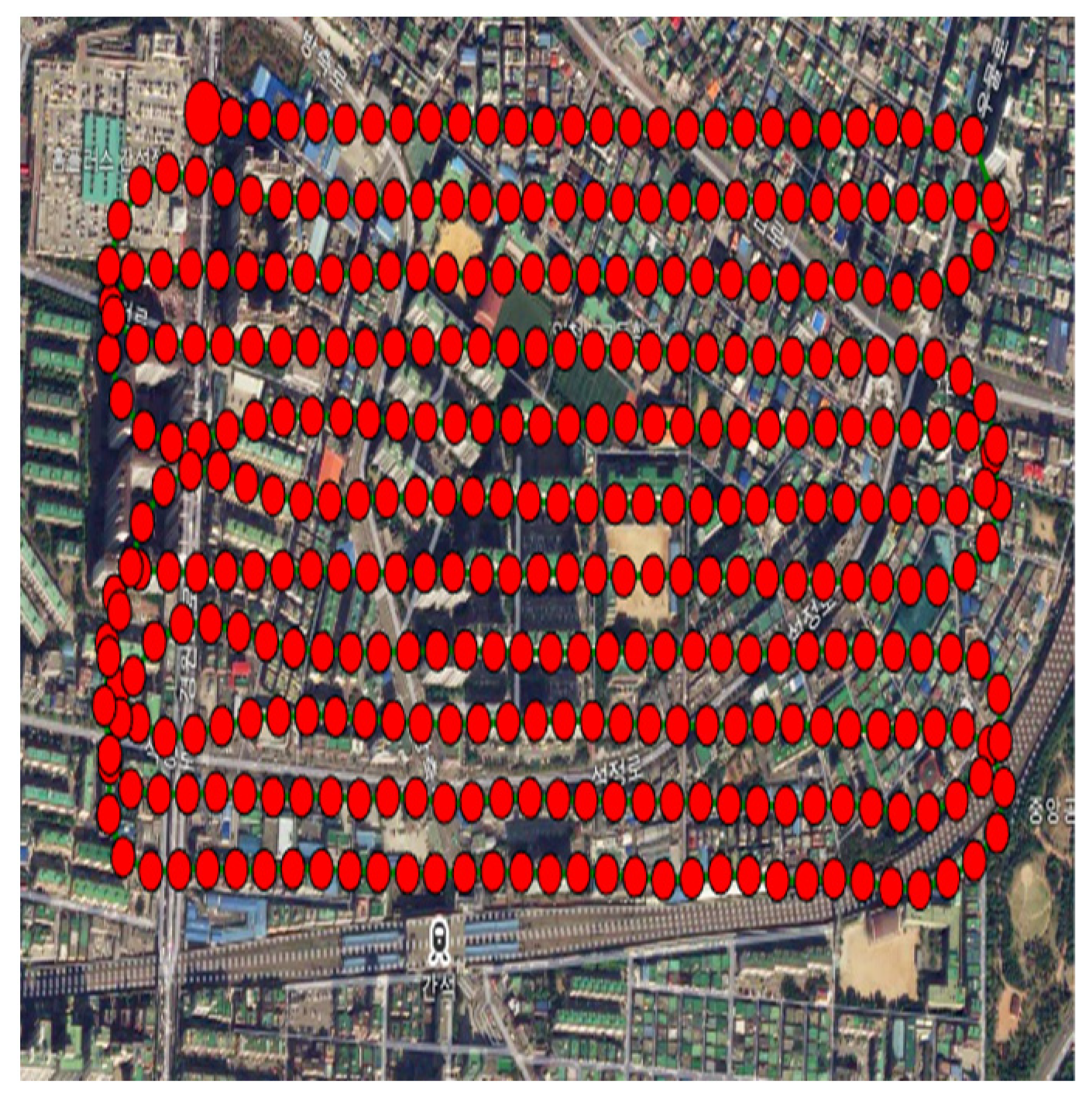
The study area selected was downtown Incheon, Korea, which has various roads, buildings and houses. A total of 362 UAV images were collected using a Firefly6 Pro. The number of strips created was 11, and the flight altitude of the UAV was 214 m. The ground sampling distance (GSD) for the images was 5.0 cm. For a precise bundle adjustment and accuracy check, five GCPs and four checkpoints (CPs) were obtained through a GPS/RTK survey.

3.2. Image Grouping and Initial-Pair Composition

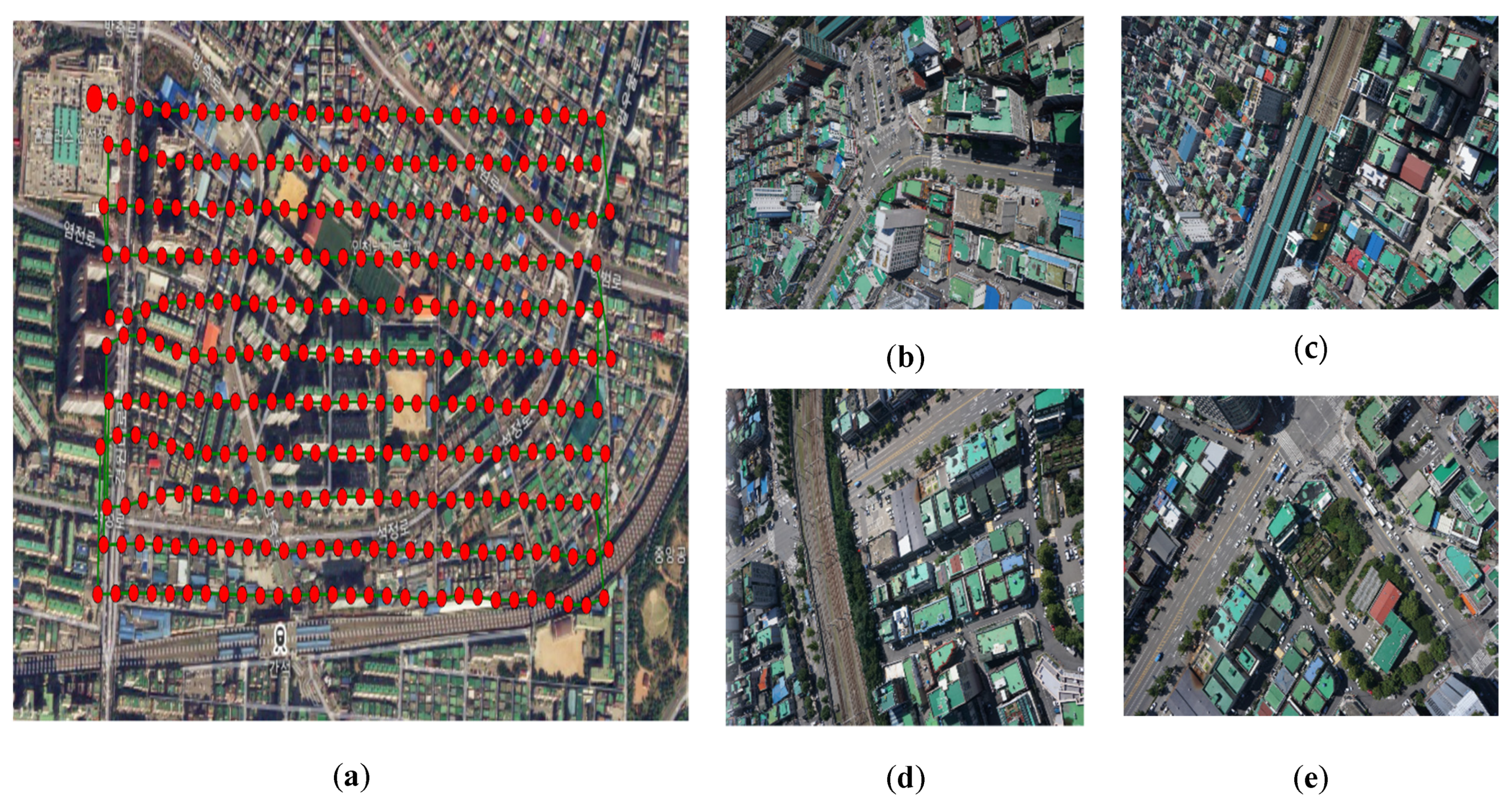
The image grouping process was applied to the 362 images based on an angular threshold of 30 degrees. If the number of images within a strip was less than five, the images were removed from further processing. Table 1 shows the results of image grouping into image sequences. Start index and end index mean the starting and ending images of each strip, with 11 strips classified from 301 of the 362 images used for final composing of the strips. On average, 27 images were grouped within a strip, after 61 images were removed because they were on the boundaries of valid strips.
Figure 8 and Figure 9 show the results from total of flight path and image grouping. Compared to Figure 8, Figure 9a shows that images on the boundaries of strips were removed successfully. Removed images were mostly oblique, because the UAV changed pose for the next strip, as shown in Figure 9b–e.
Overlaps between images within an image strip were calculated, and initial image pairs were defined. We used 5 degrees and 45 degrees as the lower and upper limits for a valid range of convergence angles, an average magnitude of two pixels was the upper limit for allowable Y-parallax, and a ratio of 20% was the lower limit for overlaps between two images. The number of pair sets and initial-image pairs for all strips are shown in Table 1.

3.3. Optimal Image-Pair Selection

We separately applied optimal-pair selection based on two selection criteria. The first criterion was to select the minimum number of pairs covering the ROI. The second was to select image pairs with the best accuracy.
Table 2 shows the results of the initial image–pair composition for Strip 1 in detail. Twenty-six pair sets were defined, and a total of 80 initial image pairs were formed. The table also shows the overlap ratio and Y-parallax error for each image pair. In Pair-Set 1, for example, image 1 had an overlap of 66% with image 2. The magnitude of the Y-parallax between images 1 and 2 was 0.6 pixels.
The optimal image–pair selection process was tested based on the first selection criterion. The starting pair was 1–2. The next pair selected was the pair overlapping 1–2 at the far-most pair set. The pairs selected based on this criterion were 1–2, 5–6, 7–8, 10–11, 13–14, 16–17, 19–20, 23–24 and 26–27 (shown in red). The selected optimal pairs are shown in the table in bold. Out of 26 pair sets, nine pairs were sufficient to cover the ROI of the strip.
Next, the optimal image–pair selection process was tested based on the second selection criterion. The magnitude of the Y-parallax between stereo images was used as the accuracy measure. The pairs selected under this criterion were 1–2, 4–5, 6–7, 9–10, 12–13, 13–14, 15–16, 16–17, 19–20, 20–21, 22–24, 24–25 and 26–27. They are underlined in the table. Out of 26 pair sets, 13 were selected as the most accurate.
The other 10 strips were processed separately using the same two selection criteria. In each strip, initial-image pairs were formed, and optimal pairs were selected. Table 3 summarizes the results of optimal-pair selection. In reference to the proposed optimal selections, we include selecting all adjacent image pairs.
Table 3 shows the results of adjacent-pair selection, minimum-pair selection and most accurate–pair selection per strip. The total number of pairs under adjacent pair selection was 290 for all 11 image strips. This indicates that 290 pairs would be processed from among the original 362 images without any intelligent pair-selection process. The average magnitude for Y-parallax for this case was 0.71 pixels.
The total number of pairs from the minimum-pair selection was 101 for all strips. Compared to adjacent-pair selection, the number of pairs was reduced greatly. A significant amount of time can be saved in stereoscopic processing of the dataset under this selection criterion. The average magnitude for Y-parallax in this case was 0.73, slightly less than the first case.
The total number of pairs from the most accurate–pair selection was 148 for all strips. Compared to minimum-pair selection, the number of pairs increased. However, this is still a great reduction, compared to adjacent-pair selection. It is notable that the average Y-parallax in this case was 0.58 pixels. Stereoscopic processing in this case should generate the most accurate results with a reduced number of pairs.

3.4. Performance of Stereoscopic Processing

Digital surface models (DSMs) and ortho-mosaic images were generated from all three cases to evaluate the performance of the proposed optimal-pair selections. For DSM generation, a stereo-matching algorithm developed in-house was used [22,23]. Stereo matching was applied to all stereo pairs in each case, and 3D points from stereo matching were allocated to DSM grids. Points in each DSM grid were averaged. Ortho-mosaics were generated using the DSMs from the three cases. For each ortho-mosaic grid, a height value was obtained from the DSM. This 3D point was then back-projected to multiple original UAV images. We chose the back-projected image pixel that was closest to the image center as the corresponding image pixel to the ortho grid.
Figure 10 shows the results of DSM and ortho-mosaic generation. In it, parts (a) and (b) were generated via adjacent-pair selection, (c) and (d) by minimum-pair selection and (e) and (f) with most accurate–pair selection. All three datasets covered the ROI without leaving any inner holes. Slight shrinking of the processed areas was observed for the second and third datasets. However, shrunken regions were due to removed image pairs, which were outside the ROI.
Table 4 shows the processing times for all types of pair selection. Case 1, which had the largest number of pairs, took the most time. On the other hand, Case 2 with the smallest number of pairs took the least time. As the number of pairs was reduced, processing time was also reduced.
For accuracy analysis, we overlapped the GCPs which were used during bundle adjustment, and the CPs, which were not used during bundle adjustment, onto the ortho-mosaic maps and the DSMs of the three datasets. Horizontal and vertical accuracy were analyzed, and Table 5 shows the results, in which the row labeled Model shows the accuracy of the GCPs, whereas the row labeled Check shows the accuracy of the CPs.
The results in Table 5 support the image-selection strategy proposed here. Note that all three cases used the same EOPs, processed with Pix4D software. Model accuracy and Check accuracy were in a similar range for all three cases. This indicates that the modeling process by Pix4D did not clear any bias. The results in Case 1 and Case 2 are in a similar range. This indicates that the minimum pair–selection criterion could successfully replace adjacent-pair selection. It is promising that the accuracy in Case 3 was lower than the others. The proposed criteria for most accurate–pair selection have been proven influential.
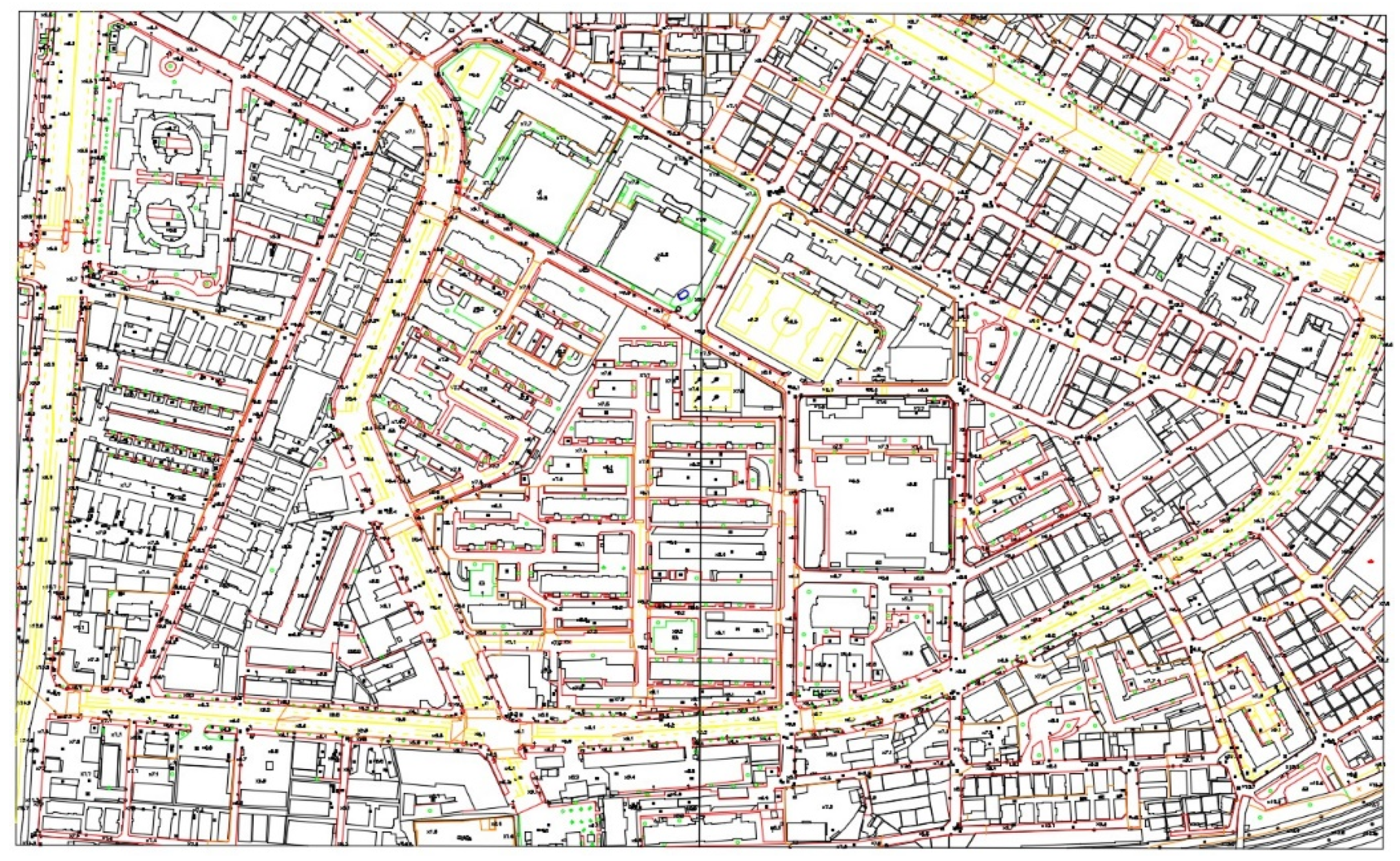
A digital map at 1:1000 scale was generated through stereoscopic plotting with the dataset from most accurate–pair selection [24]. As shown in Figure 11, large-scale maps could be generated successfully with a reduced number of images.
Table 6 shows the result of most accuracy pairs for agricultural and costal region by using fixed and rotary wings. It was confirmed that the number of most accurate pairs in all regions was reduced by about one-third compared to the input pairs. In addition, the RMSE of Y-parallax was measured to be less than 1.0 pixel, which makes it possible to generate stable stereoscopic plotting.

4. Conclusions

In this study, we proposed an intelligent pair-selection algorithm for stereoscopic processing of UAV images. We checked overlaps between stereo pairs and Y-parallax errors in each stereo pair, and we selected image pairs according to predefined selection criteria. In this paper, we defined two criteria: the minimum number of pairs and the most accurate pairs, because it is difficult to find other methods such as optimal pair composition paper. Other selection criteria are open, depending on users’ needs.
Both criteria tested could reduce the number of image pairs to cover the ROI, and hence, reduce processing time greatly. This reduction did not lead to any image loss of the processed area. Through accuracy analysis using ground control points, we verified the validity of the proposed criteria. The minimum-selection criterion showed accuracy similar to conventional adjacent-pair selection with a large redundancy. This shows that the ROI can be successfully covered with a minimum number of pairs, and that the minimum-selection criterion could replace adjacent-pair selection. Notably, the criterion proposed for most accurate–pair selection greatly reduced horizontal and vertical errors, compared to both adjacent- and minimum-pair selection. This shows that the proposed criterion could indeed be used for accurate and cost-effective stereoscopic mapping of UAV images.
Due to data availability, we used images taken in linear strips. We also assumed that the image sequence was ordered according to the image acquisition time. One may adapt our image grouping method to handle other types of strips or unordered images. In this paper, we considered image-pair reduction only within the same strip. An interesting research topic would be to extend the image-selection criteria to pair images from different strips.

Author Contributions

Conceptualization, P.-c.L. and T.K.; Data curation, P.-c.L., J.S., J.-I.K. and J.C.; Formal analysis, P.-c.L., S.R., J.-I.K. and T.K.; Funding acquisition, J.-I.K., J.C. and T.K.; Investigation, J.S., J.-I.K. and S.-b.L.; Methodology, P.-c.L., S.R., J.-I.K. and T.K.; Project administration, J.-I.K. and J.C.; Software; Supervision, T.K.; Validation, P.-c.L., S.-b.L. and T.K.; Visualization, P.-c.L. and J.S.; Writing—review and editing, T.K. All authors have read and agreed to the published version of the manuscript.

Funding

Polar Industrial Program of Korea Polar Research Institute (grant number: PE 21910).

Conflicts of Interest

The authors declare they have no conflict of interest.

References

  1. Park, Y.; Jung, K. Availability evaluation for generation of geospatial information using fixed wing UAV. J. Korean Soc. Geospat. Inform. Syst. 2014, 22–24, 159–164. [Google Scholar]
  2. Lim, P.C.; Seo, J.; Son, J.; Kim, T. Feasibility study for 1:1000 scale map generation from various UAV images. In Proceedings of the International Symposium on Remote Sensing, Taipei, Taiwan, 17–19 April 2019. Digitally available on CD. [Google Scholar]
  3. Radford, C.R.; Bevan, G. A calibration workflow for prosumer UAV cameras. Int. Arch. Photogram. Remote Sens. Spat. Inform. Sci. 2019, XLII-2/W13, 553–558. [Google Scholar] [CrossRef] [Green Version]
  4. Rhee, S.; Hwang, Y.; Kim, S. A study on point cloud generation method from UAV image using incremental bundle adjustment and stereo image matching technique. Korean J. Remote Sens. 2019, 34, 941–951. [Google Scholar]
  5. Zhou, Y.; Rupnik, E.; Meynard, C.; Thom, C.; Pierrot-Deseilligny, M. Simulation and Analysis of Photogrammetric UAV Image Blocks—Influence of Camera Calibration Error. Remote Sens. 2019, 12, 22. [Google Scholar] [CrossRef] [Green Version]
  6. Cucci, D.A.; Rehak, M.; Skaloud, J. Bundle adjustment with raw inertial observations in UAV applications. ISPRS J. Photogram. Remote Sens. 2017, 130, 1–12. [Google Scholar] [CrossRef]
  7. Wohlfeil, J.; Grießbach, D.; Ernst, I.; Baumbach, D.; Dahlke, D. Automatic camera system calibration with a chessboard enabling full image coverage. Int. Arch. Photogramm. Remote Sens. Spat. Inf. Sci. 2019, 42, 1715–1722. [Google Scholar] [CrossRef] [Green Version]
  8. Choi, Y.; You, G.; Cho, G. Accuracy analysis of UAV data processing using DPW. J. Korean Soc. Geospat. Inform. Sci. 2015, 23, 3–10. [Google Scholar]
  9. Dai, Y.; Gong, J.; Li, Y.; Feng, Q. Building segmentation and outline extraction from UAV image-derived point clouds by a line growing algorithm. Int. J. Digit. Earth 2017, 10, 1077–1097. [Google Scholar] [CrossRef]
  10. Kim, J.I.; Kim, T.; Shin, D.; Kim, S. Fast and robust geometric correction for mosaicking UAV images with narrow overlaps. Int. J. Remote Sens. 2017, 38, 2557–2576. [Google Scholar] [CrossRef]
  11. Kim, J.I.; Hyun, C.U.; Han, H.; Kim, H.C. Evaluation of Matching Costs for High-Quality Sea-Ice Surface Reconstruction from Aerial Images. Remote Sens. 2019, 11, 1055. [Google Scholar] [CrossRef] [Green Version]
  12. Maini, P.; Sujit, P.B. On cooperation between a fuel constrained UAV and a refueling UGV for large scale mapping applications. In Proceedings of the International Conference on Unmanned Aircraft Systems, Denver, CO, USA, 9–12 June 2015; pp. 1370–1377. [Google Scholar]
  13. Shin, J.; Cho, Y.; Lim, P.; Lee, H.; Ahn, H.; Park, C.; Kim, T. Relative Radiometric Calibration Using Tie Points and Optimal Path Selection for UAV Images. Remote Sens. 2020, 12, 1726. [Google Scholar] [CrossRef]
  14. Brown, M.; Lowe, D.G. Automatic panoramic image stitching using invariant features. Int. J. Comp. Vis. 2017, 74, 59–73. [Google Scholar] [CrossRef] [Green Version]
  15. Kim, J.I. Development of a Tiepoint Based Image Mosaicking Method Considering Imaging Characteristics of Small UAV. Ph.D. Thesis, Inha University, Incheon, Korea, 2017. [Google Scholar]
  16. Kim, J.I.; Kim, T. Precise rectification of misaligned stereo images for 3D image generation. J. Broadcast Eng. 2012, 17, 411–421. [Google Scholar] [CrossRef]
  17. Kim, J.I.; Kim, H.C.; Kim, T. Robust Mosaicking of Lightweight UAV Images Using Hybrid Image Transformation Modeling. Remote Sens. 2020, 12, 1002. [Google Scholar] [CrossRef] [Green Version]
  18. Jung, J.; Kim, T.; Kim, J.; Rhee, S. Comparison of Match Candidate Pair Constitution Methods for UAV Images Without Orientation Parameters. Korean. J. Remote Sens. 2016, 32, 647–656. [Google Scholar]
  19. Son, J.; Lim, P.C.; Seo, J.; Kim, T. Analysis of bundle adjustments and epipolar model accuracy according to flight path characteristics of UAV. Int. Arch. Photogram. Remote Sens. Spat. Inf. Sci. 2019, 607–612. [Google Scholar] [CrossRef] [Green Version]
  20. Jeong, J.; Kim, T. Analysis of dual-sensor stereo geometry and its positioning accuracy. Photogram. Eng. Remote Sens. 2014, 80, 653–661. [Google Scholar] [CrossRef]
  21. Jeong, J.; Yang, C.; Kim, T. Geo-positioning accuracy using multiple-satellite images: IKONOS, QuickBird, and KOMPSAT-2 stereo images. Remote Sens. 2015, 7, 4549–4564. [Google Scholar] [CrossRef] [Green Version]
  22. Haines, E. Point in polygon strategies. Graph. Gems IV 1994, 994, 24–26. [Google Scholar]
  23. Yoon, W.; Kim, H.G.; Rhee, S. Multi point cloud integration based on observation vectors between stereo images. Korean J. Remote Sens. 2019, 35, 727–736. [Google Scholar]
  24. Lee, S.B.; Kim, T.; Ahn, Y.J.; Lee, J.O. Comparison of Digital Maps Created by Stereo Plotting and Vectorization Based on Images Acquired by Unmanned Aerial Vehicle. Sens. Mater. 2019, 31, 3797–3810. [Google Scholar] [CrossRef]
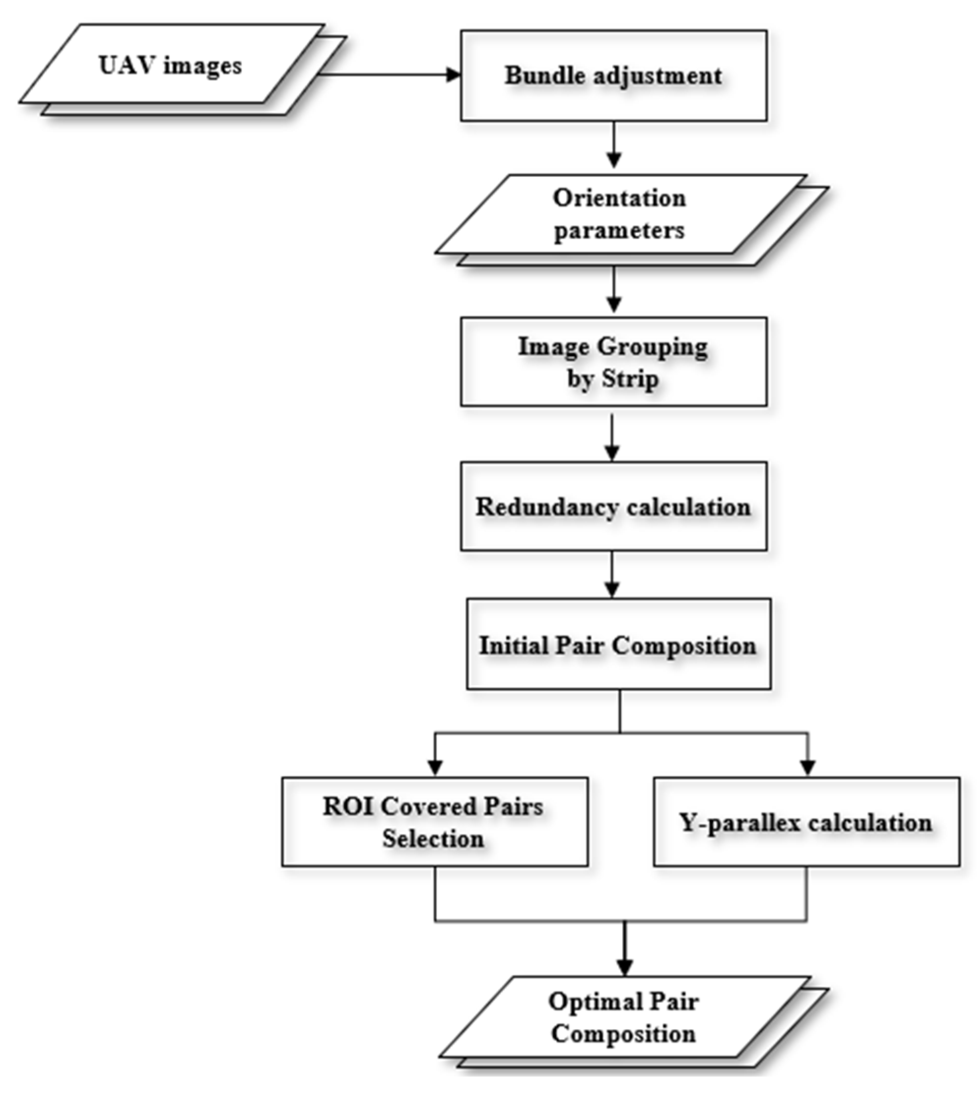
Figure 1. Overall flow chart of optimal pair selection.
Remotesensing 13 02118 g001
Figure 2. Example of image grouping (top) and its results (bottom).
Remotesensing 13 02118 g002
Figure 3. An overlap area in ground space.
Remotesensing 13 02118 g003
Figure 4. Example of the pair sets in a strip with six images.
Remotesensing 13 02118 g004
Figure 5. The first iteration for optimal pair composition in a strip.
Remotesensing 13 02118 g005
Figure 6. The overlap between the polygons generated from each pair.
Remotesensing 13 02118 g006
Figure 7. The second iteration for optimal pair composition in a strip.
Remotesensing 13 02118 g007
Figure 8. Top view of the flight path of the UAV (green line) and the locations of the images acquired (red dots).
Remotesensing 13 02118 g008
Figure 9. (a) Top view of UAV image positions and (be), images 57 to 60, which were removed after strip classification.
Remotesensing 13 02118 g009
Figure 10. Digital surface models (left) and ortho-mosaic images (right) generated by each type of pair selection: (a,b) were generated by adjacent-pair selection; (c,d) were generated by minimum-pair selection; while (e,f) were generated with most accurate–pair selection.
Remotesensing 13 02118 g010
Figure 11. A digital map generated by stereoscopic plotting with most accurate pairs.
Remotesensing 13 02118 g011
Table 1. The results of image grouping into strips.
StripStart Index
of Image
End Index
of Image
Number of ImagesNumber of
Pair-Sets
Number of
Pairs
1127272686
23459262579
36792262577
499124262577
5133158262577
6164192292882
7199226282781
8234259262576
9268295282780
10299328302987
11334362292882
Total Number301290884
Table 2. Initial-image pairs and the results of optimal-image selection for the first strip (red font: the minimum pairs; underline: the best accuracy pairs). Each cell shows an image ID with overlap ratio and magnitude of Y-parallax error in parentheses.
Pair-Set 1Pair-Set 2Pair-Set 3Pair-Set 4Pair-Set 5Pair-Set 6Pair-Set 7
1–2 (66, 0.6)2–3 (84, 1.0)3–4 (85, 0.7)4–5 (84, 0.4)5–6 (72, 1.0)6–7 (76, 0.6)7–8 (73, 0.8)
1–3 (51, 0.7)2–4 (68, 1.0)3–5 (73, 0.7)4–6 (58, 1.1)5–7 (51, 0.7)6–8 (50, 0.9)7–9 (43, 0.8)
1–4 (38, 1.1)2–5 (57, 1.1)3–6 (46, 1.2)4–7 (39, 0.6)5–8 (30, 1.6)6–9 (22, 1.0)7–10 (22, 1.0)
1–5 (28, 3.2)2–6 (36, 2.4)3–7 (26, 0.8)
Pair-Set 8Pair-Set 9Pair-Set 10Pair-Set 11Pair-Set 12Pair-Set 13Pair-Set 14
8–9 (69, 0.8)9–10 (77, 0.7)10–11 (74, 3.8)11–12 (72, 0.5)12–13 (81, 0.4)13–14 (76, 0.4)14–15 (78, 0.7)
8–10 (47, 1.0)9–11 (54, 2.9)10–12 (49, 3.7)11–13 (58, 0.5)12–14 (59, 0.5)13–15 (57, 0.7)14–16 (51, 0.8)
8–11 (27, 0.8)9–12 (30, 2.8)10–13 (35, 3.3)11–14 (39, 0.7)12–15 (40, 0.8)13–16 (33, 0.8)14–17 (29, 1.0)
Pair-Set 15Pair-Set 16Pair-Set 17Pair-Set 18Pair-Set 19Pair-Set 20Pair-Set 21
15–16 (72, 0.4)16–17 (76, 0.5)17–18 (76, 0.7)18–19 (79, 0.6)19–20 (72, 0.5)20–21 (78, 0.6)21–22 (75, 0.8)
15–17 (48, 0.6)16–18 (53, 0.7)17–19 (58, 1.1)18–20 (53, 1.1)19–21 (54, 0.7)20–22 (63, 0.8)21–23 (56, 1.5)
15–18 (26, 0.6)16–19 (35, 0.9)17–20 (32, 1.9)18–21 (36, 1.1)19–22 (38, 0.9)20–23 (36, 1.6)21–24 (37, 1.1)
18–22 (20, 2.2) 20–24 (25, 0.7)
Pair-Set 22Pair-Set 23Pair-Set 24Pair-Set 25Pair-Set 26
22–23 (69, 1.3)23–24 (75, 1.0)24–25 (71, 0.7)25–26 (70, 1.7)26–27 (74, 1.1)
22–24 (61, 0.7)23–25 (48, 0.9)24–26 (48, 1.7)25–27 (48, 1.2)
22–25 (32, 0.8)23–26 (33, 2.0)24–27 (25, 1.8)
Table 3. Results of optimal adjacent-, minimum-, and geometric-pair composition for each strip.
StripCase 1.
Adjacent—Pair
Selection
Case 2.
Minimum—Pair
Selection
Case 3.
Most Accurate—Pair
Selection
Number
of Pairs
Y-Parallax
(Pixels)
Number
of Pairs
Y-Parallax
(Pixels)
Number
of Pairs
Y-Parallax
(Pixels)
1260.8090.90130.61
2250.6190.56120.51
3250.7080.88130.55
4250.61110.76140.53
5250.7770.80120.61
6280.70100.60120.50
7270.7490.65140.58
8250.7590.72150.64
9270.75100.80150.66
10290.74100.55150.51
11280.7190.84120.63
Avg260.7190.73130.58
Total290-101-148-
Table 4. Resulting processing times for all types of pair selection.
Type of
Product
Case 1.
Adjacent—Pair
Selection
Case 2.
Minimum—Pair
Selection
Case 3.
Most Accurate—Pair Selection
Stereo
matching
100 min38 min57 min
DSM and
Ortho-mosaic
15 min7 min9 min
Total
processing time
115 min45 min66 min
Table 5. Accuracy analysis results of DSMs and ortho-mosaic images.
AccuracyCase 1. Adjacent Pair
Selection
Case 2. Minimum Pair
Selection
Case 3. Most Accurate Pair
Selection
Horizontal
(cm)
Vertical
(cm)
Horizontal
(cm)
Vertical
(cm)
Horizontal
(cm)
Vertical
(cm)
Model8.425.25.522.86.17.4
Check8.218.37.224.25.97.5
Table 6. Most accurate pair composition result for each region.
Study
Region
Type of
UAV
Number of
Strip
Number of
Input Images
Number of
Most Accurate Pairs
Y-Parallax
RMSE
(Pixel)
AgriculturalFixed-wings659180.84
CostalRotary-wings695260.88
AgriculturalRotary-wings651150.55
Publisher’s Note: MDPI stays neutral with regard to jurisdictional claims in published maps and institutional affiliations.