Extrapolating Satellite-Based Flood Masks by One-Class Classification—A Test Case in Houston

Abstract

Flood masks are among the most common remote sensing products, used for rapid crisis information and as input for hydraulic and impact models. Despite the high relevance of such products, vegetated and urban areas are still unreliably mapped and are sometimes even excluded from analysis. The information content of synthetic aperture radar (SAR) images is limited in these areas due to the side-looking imaging geometry of radar sensors and complex interactions of the microwave signal with trees and urban structures. Classification from SAR data can only be optimized to reduce false positives, but cannot avoid false negatives in areas that are essentially unobservable to the sensor, for example, due to radar shadows, layover, speckle and other effects. We therefore propose to treat satellite-based flood masks as intermediate products with true positives, and unlabeled cells instead of negatives. This corresponds to the input of a positive-unlabeled (PU) learning one-class classifier (OCC). Assuming that flood extent is at least partially explainable by topography, we present a novel procedure to estimate the true extent of the flood, given the initial mask, by using the satellite-based products as input to a PU OCC algorithm learned on topographic features. Additional rainfall data and distance to buildings had only minor effect on the models in our experiments. All three of the tested initial flood masks were considerably improved by the presented procedure, with obtainable increases in the overall $\kappa$ score ranging from 0.2 for a high quality initial mask to 0.7 in the best case for a standard emergency response product. An assessment of $\kappa$ for vegetated and urban areas separately shows that the performance in urban areas is still better when learning from a high quality initial mask.

1. Introduction

Satellite-based flood mapping is a central topic in applied remote sensing, due to the high relevance of accurate event maps in all phases of the disaster risk management cycle. Besides the use during emergency response, the observed flood extent is often necessary for post-event analysis, including modelling studies. An emerging field is also the assimilation of flood extents in near-real-time into hydrodynamic models [1]. The term flood mask refers to a binary geospatial data layer of flood water extent, where the permanent water bodies are excluded. Most products are currently based on synthetic aperture radar (SAR) sensors, which can operate day and night, independent of cloud cover. As the temporal coverage and free-of-charge availability of satellite imagery steadily increases, flood masks of varying quality and file format are produced, for example, by the Copernicus Emergency Management Service of the European Commission (EMSR). However, there are still obvious limitations to these currently available products, which hamper their usage: (1) Urban flooding is usually underdetected, because built-up areas are difficult to observe from space, due to the occurrence of radar shadows, layover effects, and speckle (e.g., [2,3]). This is for example problematic for damage estimations, which are strongly influenced by the number of exposed buildings within the flood mask [4]; (2) Flooding below the vegetation canopy, although theoretically detectable on longer wavelength sensors depending on the density of the canopy [5,6], is typically omitted as well, even along river courses, which obscures the true land-water boundary. Algorithms for deriving the water depth from a mapped extent are available, but hinge on the precision of that land-water boundary [7,8,9,10] as well as on the quality of the elevation data [11]. Inundation depth is often required in applications, for example flood damage models usually rely on it as main explanatory feature (exceptions being crop damage models, which may use duration and timing). Therefore, a step towards more reliable flood extent is also a step towards the applicability in hydrodynamic and flood damage models; (3) The often undescribed uncertainty of satellite-based flood masks leads to further problems in applications, for example, when assessing the performance of a hydraulic model [12]. Although some scientific studies provide uncertainty estimates (e.g., [13,14]), this is not yet operational standard, for example, for the EMSR products.

A staggering amount of different methods has already been explored for water delineation from SAR images. Examples include automatic grey level thresholding [15], active contour models [16], fuzzy scoring [17,18], time series analysis [19], Bayesian networks [20] and, recently, convolutional neural networks [21,22]. Nevertheless, the information content of single-date, single-polarization SAR amplitude data is limited in vegetated and especially in urban environments, which are the most interesting areas with respect to impact estimations. Acknowledging these limitations, the remote sensing community moves towards integration of additional information layers, such as interferometric coherence [3,20,23], optical data [24], terrain elevation [2,25,26] and even social media content [27]. The cited approaches incorporating topographic information use this mainly to exclude false positives. Most notably for this study, a typical postprocessing step is to overlay the classified flood extent with so-called exclusion layers, to reduce false positives from material that exhibits low backscatter, like dry sand [28]. With this in mind, we conclude that flood masks from SAR data can be optimized to reduce false positives, by sophisticated classification methods and exclusion layers, but cannot avoid false negatives in areas which are unobservable for the sensor, for example, due to the abovementioned effects.

The hydrological and geomorphological communities have developed advanced GIS approaches to delineate flood-prone areas without having to resort to numerical hydraulic models [29,30,31], also with a focus on urban areas [32,33]. While numerical models still have many advantages, and benefit from the increase of computation power, they require bathymetry and discharge or water level as boundary condition, which is not always available. Examples of indicators that have successfully been used in the context of flood susceptibility mapping, for example, in the cited studies above, are the Height Above Nearest Drainage (HAND) index [34] and the Topographic Wetness Indicator (TWI) [35]. In the following, we investigate whether these and other geomorphological features, precipitation, and distance to buildings, are suitable to identify flooded areas, which are not detected on remote sensing products. The approach consists of using a satellite-based flood mask as training area for a machine learning algorithm. The basic research question is: “if this is the satellite-based flood mask, where then should we expect water in reality?”.

This question can be expressed as a supervised learning task, in which the labels necessary for training are taken from the initial mask. Supervised models are able to learn complex relationships from the explanatory features by optimizing an objective function that penalizes misclassification of the provided labels in the training samples. However, correct labels are required for training. Regular binary classifiers require positive and negative (PN) examples. We argue in this paper that positive and unlabeled (PU), rather than PN, is the appropriate description of state-of-the-art satellite-based flood masks, as long as the limitations of these masks are not clearly communicated, for example, in a validity layer. This leads us to formulate our research question as a one-class classification (OCC) problem. OCC algorithms require only one class to be labeled, termed the positive (P) class. They may use either only P or PU training data, thereby avoiding to wrongly treat unknown labels as true negatives. Such methods are commonly used in habitat modelling [36] as well as for specific remote sensing questions like mapping raised bogs [37], invasive tree species [38], Bark Beetle infestation [39] or damaged maize fields [40]. Mack & Waske [41] investigated the discriminative power of the well-known PU algorithms MaxEnt [36] and Biased Support Vector Machine (BSVM, [42]) in comparison to a P classifier and a PN benchmark model for a variety of classification tasks. PU learning is generally considered more promising than P learning, especially when classes are not perfectly separable, because PU algorithms may learn about the overall distributional characteristics. When using an OCC on satellite-based flood masks, there is no need for a validity layer, as long as false positives have been minimized during the creation of the flood mask (depending on the algorithm, some violation of this assumption is acceptable).

The aim of this study is to improve satellite-based flood masks by reducing false negatives in areas where the satellite sensor has low sensitivity, such as vegetated and urban areas. Our investigation requires a flood event covered by multiple satellite-based flood masks of different quality, relatively high resolution topography, gridded rainfall measurements, and mapped building footprints. Additionally, we use high-quality flood extent maps (“ground truth”) for testing the performance of the proposed approach. We chose the well-documented event of 2017 hurricane Harvey in Houston, TX, as test case. We present a novel methodology for extrapolation by OCC and test it with three different initial satellite-based masks on different spatial scales. The paper is organized as follows: Section 2 gives a description of the flood event and used datasets, followed by details on the algorithms, performance metrics, and experimental setup. In Section 3, the skill of the BSVM and MaxEnt models is compared, and the effect of a region-growing postprocessing is quantified. Example maps of spatial predictions are shown for selected models. The results are then discussed in a broader context in Section 4.

2. Materials & Methods

2.1. Study Area and Datasets

Hurricane Harvey ranks among the costliest disasters that have affected the United States during the last decades [43], with Houston in particular suffering severe damage in the final days of August 2017. Although considered primarily a pluvial flood event, with implications for modelling [44], the vast spatial extent and long duration of the rainfall also caused all major river basins to overflow. According to the Harris County Flood Control District (HCFCD), 70,370 out of 154,170 flooded homes were located beyond the official 500-year flood hazard zone [45]. Water levels in the San Jacinto River exceeded all historical records, with estimated return periods above 500 years in many places. In the western part of Houston, two large-scale flood control structures, the Barker reservoir and the Addicks reservoir (Figure 1) were forced to open their release gates on 28 August, but the water level within continued to rise until August 30 to the point of local overtopping, despite the open gates [46]. The combined outflow of both reservoirs led to a massive flooding of the Buffalo Bayou. It is reported that about 14,000 homes were even located within the reservoirs themselves.

2.1.1. Flood Masks for Training and Validation

The following products were used in our study as initial flood masks for training the OCC models: The EMSR released a mapping of areas inundated by Hurricane Harvey on 31 August 2017 (EMSR_229), based on Cosmo-SkyMed data. This is a typical standard product, designed for rapid response. The EMSR_229 mask covers the entire urban area of Houston and surroundings. Li et al. [20] further classified parts of a Sentinel-1 scene from August 30th, including interferometric coherence with previous scenes, by a Bayesian Network fusion technique (DLR_BN). Li et al. [21] also processed TerraSAR-X images by a convolutional neural network (DLR_CNN), with the flooded scene dating to September 1st. The latter is only available for a rather small region within the city, along the Buffalo Bayou. Both DLR_BN and DLR_CNN can be regarded as “high quality” masks, with reported $\kappa$ coefficients of 0.68 in both cases from comparison to a labeled aerial image. However, we observed some flaws in this labeling when comparing it to the raw aerial image.

Validation in our study is based on two independent products: First, we downloaded the original 50 cm resolution aerial image acquired by the National Oceanic and Atmospheric Administration (NOAA) on 30 August 2017, accessed on 3 December 2020. (https://storms.ngs.noaa.gov/storms/harvey/index.html#9/29.8430/-95.0729) and manually labeled all flooded areas on the image (NOAA_labeled) in three categories: open flood water, flooded vegetation, and flooded urban area. The land cover classes allow for calculating the model skill in a stratified manner, providing numbers for vegetated and urban areas separately. The guiding principle for assigning these land cover classes was to consider what is visible from the point of view of a satellite. Small patches of open water within built-up environment were still labeled “urban”, as the SAR signal in these locations would most likely be influenced by the surrounding buildings. The main channel of the Buffalo Bayou was labeled “vegetation”, as there are mainly tree canopies visible from a satellite’s perspective. Great care was taken to only include buildings in this reference map where it was obvious, for example, from the color of the swimming pools, that at least the ground floor of the building got affected—otherwise we only delineated the visible water on the roads. Permanent lakes within the urban areas were intentionally not mapped, only the flood waters surrounding the regular lake extents. While some residual ambiguity remained between the assigned land cover classes, especially between open water and flooded vegetation inside the large reservoirs, we are confident that this manually labeled image is a very precise reference for the situation on 30 August 2017. This reference map is publicly available as online supplement to this publication. Secondly, we obtained a mapping by the United States Geological Survey (USGS) for the San Jacinto River (USGS_SJ). The USGS has released flood extents for major river catchments [47], based on interpolated field measurements of high water marks (HWM), which have been used by the company Fathom [44] as “ground-truth” for validating their hydraulic model simulation of the event. Watson et al. [47] acknowledge that some uncertainties remain in areas where the coverage of the HWM is sparse and that the mapped boundary was manually extended to anthropogenic structures such as roads or bridges. We overlayed all masks with OpenStreetMap (OSM) water layer (http://hydro.iis.u-tokyo.ac.jp/~yamadai/OSM_water/, accessed on 20 July 2020), which includes categorized water bodies in high spatial detail, and removed all of these areas from the masks, thereby equally converting all masks to flood masks.

2.1.2. Explanatory Features

An overview of used datasets and features is given in

Table 1. Flood masks for training and validation.

Floodmask	Data Source	Date of Image	Resolution	Usage
EMSR_229	Cosmo-SkyMed	31 August 2017	30 m	Training
DLR_BN	Sentinel-1	30 August 2017	15 m	Training
DLR_CNN	TerraSAR-X	1 September 2017	40 m (32 × 1.25)	Training
NOAA_labeled	Aerial image	30 August 2017	0.5 m	Validation
USGS_SJ	HWM	Maximum extent	3 m	Validation

and

Table 2. Datasets and features.

Feature	Data Source	Category
HAND_large_lake_river	NED + OSM	Topo
HAND_major_river	NED + OSM	Topo
HAND_small_stream_canal	NED + OSM	Topo
Dist_large_lake_river	OSM	Topo
Dist_major_river	OSM	Topo
Dist_small_stream_canal	OSM	Topo
Slope	NED	Topo
Curvature	NED	Topo
TWI	NED	Topo
TPI 11x11	NED	Topo
TPI 51x51	NED	Topo
TPI 101x101	NED	Topo
Rainfall_sum	NWS	Rain
Rainfall_acc	NWS + NED	Rain
Dist_to_buildings	Microsoft USBuildingFootprints	Buildings

. A digital elevation model (DEM) called the National Elevation Dataset (NED) is available from the USGS, based on the best available data source per area [48]. We used the 1/3 arc seconds (~10 m) version. From the DEM, different features have been derived: slope, curvature, topographic wetness index (TWI) and topographic position index (TPI). The TPI is a geomorphological measure derived by focal window operations, which in machine learning terminology can be considered a manual convolution on the DEM. TPI has a clear physical meaning, as it indicates local hills and depressions. Combining TPI on multiple scales allows for identifying more complex landscape morphologies [49]. We used the implementation in the R library spatialEco [50] and computed TPI on the scale of 11, 51, and 101 cells, which corresponds to about 50, 250, and 500 m in all directions. The OSM water layer distinguishes 5 types of water bodies in this area, namely “Ocean”, “Large Lake & River”, “Major River”, “Small Stream” and “Canal”. We discarded the ocean and merged “Small Stream” and “Canal” as these labels appeared to have been used interchangeably from visual inspection in the Houston area. This left us with three different stream layers, for which we computed the HAND and Euclidean distance separately (by GRASS r.watershed and GDAL Proximity). OSM buildings had very limited coverage in Houston at the time of this study, therefore we used Microsoft USBuildingFootprints (https://github.com/microsoft/USBuildingFootprints, accessed on 26 August 2020). The Euclidean distance was computed on rasterized shapes, which corresponds to the distance to the closest building cell. Gridded rainfall data was downloaded from the US National Weather Service (NWS) website (https://water.weather.gov/precip/download.php, accessed on 25 August 2020). We used the sum of 26–30 August, where most of the rainfall occurred in Houston. The accumulated rainfall was computed via the GRASS GIS tool r.accumulate, with the rainfall sum as input. Features were separated into three groups for our experiments. Most features were derived from the DEM and/or stream location data, and therefore called “Topo” features. These were always used. The “Rain” and “Buildings” features were added separately to test the effect of the additional data. To keep it simple during processing, we resampled all datasets to the resolution of the DEM, so that all layers could be converted to a raster stack.

2.2. Algorithms and Performance Metrics

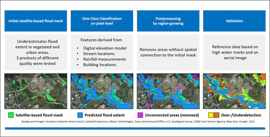
2.2.1. OCC Algorithms

Two commonly used PU learning algorithms are tested in this study for the purpose of extrapolating satellite-based flood masks from the abovementioned features. BSVM [42] is a discriminative algorithm, originally developed for text classification. It was found superior to previous multi-step OCC procedures, and also to other P and PU learners, for classification of remote sensing images [41]. Essentially, it is a support vector machine with radial basis function (RBF) kernel and unequal misclassification penalty terms in the cost function. By assigning higher penalty to misclassified positive samples, the unlabeled samples are considered “negotiable” during training. The biased cost function is given as Equation (1)

$$\begin{array}{c}\mathrm{Minimize}\frac{1}{2}{w}^{T}w+C_{+}{\displaystyle \sum _{i=1}^{k-1}}{\xi }_i+C_{-}{\displaystyle \sum _{i=k}^n}{\xi }_i\\ \mathrm{Subject}\mathrm{to}{y}_i(w^T{x}_i+b)\ge 1-{\xi }_i,i=1,2,\dots ,n\\ {\xi }_i\ge 0,i=1,2,\dots ,n,\end{array}$$

(1)

where $C_{+}$ and $C_{-}$ are the cost of misclassification for positive and unlabeled samples, respectively. $C_{+}$ is in practice parametrized by $C_{Multiplier}$ times $C_{-}$. w is the weight vector, x is the feature vector, and y is the corresponding label. $\xi$ is the slack variable used to evaluate potential hyperplanes for k−1 positive and k−n unlabeled samples. Superscript T denotes the inner product.

The so constructed hyperplane has by definition a value of 0, which can be regarded as the “default” threshold (${\theta }_{Default}$) for binary classification of BSVM. The continuous output of BSVM gives the distance to this hyperplane, where higher values indicate samples associated with the positive class (i.e., flood in our case), and lower values indicate samples associated with the negative class. However, a threshold for binary classification can be set by the user at any value, and it is sometimes recommended in the literature not to rely on the default in application, for example [41]. For the PN benchmark models, we used a regular (unbiased) support vector machine (SVM), in which the misclassification costs for both classes are equal.

MaxEnt [36] is a generative algorithm with solid roots in information theory and probabilistic reasoning [51]. The implementation in a stand-alone software, which is now open source [52], is commonly used in ecological modelling as well as for mapping rare land cover classes. The developers phrase the objective of the maximum entropy principle as estimating a distribution that agrees with everything that is known, and at the same time avoiding any assumptions about what is unknown. More specifically, the procedure searches for a Gibbs distribution, under the constraints that the expectation of every feature corresponds roughly to the empirical feature mean, while pertaining a shape as close to the prior distribution as possible. MaxEnt internally computes variance features, product features, threshold features, and hinge features. This allows the algorithm to learn complex responses and interactions, but requires regularization to avoid overfitting. The optimal value of the regularization parameter $\beta$ is accordingly determined over a grid search. Note that the original formulation by [36] is in geographic space, and in that space the prior distribution is a uniform distribution, that is, all locations are a-priori equally likely to contain the positive class. More in line with machine learning literature is the formulation in feature space, where the prior is the marginal feature distribution, and MaxEnt estimates the distribution of the positive class by minimizing the relative entropy (Kullback-Leibler divergence) between the positive and marginal distributions under the constraints imposed by the feature means [53]. The formulation is unconditional, so that only positive and unlabeled data is required. In other words, MaxEnt models the ratio of presence to background, which results in a relative probability. The cost function Equation (2), in the notation of the authors, can be shown to be the negative log-likelihood with an L1 penalty term.

$$\begin{array}{c}\mathrm{Minimize}\tilde{\pi }[-ln\left(q_{\lambda }\right)]+{\displaystyle \sum _j}{\beta }_j\left|{\lambda }_j\right|\\ \mathrm{Subject}\mathrm{to}|\widehat{\pi }\left[f_j\right]-\tilde{\pi }\left[f_j\right]|\le {\beta }_j,\end{array}$$

(2)

where $\tilde{\pi }$ is the prior distribution, $\widehat{\pi }$ the resulting MaxEnt distribution, $q_{\lambda }$ the Gibbs distribution, square brackets [] denote the expectation, ln the natural logarithm, $\beta$ is the cost parameter, and $\lambda$ the weights, over j features f.

The result of MaxEnt is a relative occurrence rate, sometimes termed “suitability”, which can be obtained in different transformed (monotonically related) output formats. Similar to [39], we use a value 0.5 on the so-called logistic output format as “default” threshold for MaxEnt, because this is the default value for the internal parameter used to create the logistic output [53]—despite strong arguments in the literature stating that this output format should not be carelessly treated as absolute probability of presence [54,55]. This theoretical issue is not of interest to us here, since we do not apply any probabilistic interpretation. For further mathematical details, the interested reader is referred to the abovementioned original literature. In this study, we relied on the R library oneClass (https://github.com/benmack/oneClass, last access on 05 October 2020), which contains a BSVM implementation, as well as an R wrapper of MaxEnt that calls the Java source file. Both implementations internally scale the data.

2.2.2. Post Processing by Region Growing

To restrict the predicted flood extent to those areas that have a spatial connection to the initial extent, we applied the ConnectedThreshold method from the Python module SimpleITK [56]. The procedure starts at given seed points and checks whether neighboring raster cell values fall within or outside a user-defined range. As seed, the original SAR-derived flood extents were used. If a cell is discarded, its neighbors are not considered and the propagation in that direction stops. When providing a binary raster (dry or flooded, denoted as 0 or 1) and setting the user-defined threshold to 1, then the result is simply a cut-back binary raster, on which all flood cells unconnected to the initial flood extent are reset to non-flooded.

2.2.3. Performance Metrics

Two different types of metrics are needed for this study: training metrics based on PU data to select the best model during the parameter grid search, and validation metrics based on the PN reference to evaluate the final extrapolations. With only positive and unlabeled data, the quantities that can reliably be estimated are the True Positives (TP, prediction and observation are positive), the False Negatives (FN, prediction misses positive observation), and the model’s probability of positive predictions among all predictions. From these quantities, various metrics have been proposed in the literature (see e.g., [57,58]). However, most of these metrics are depending on the binarization threshold. For threshold-independent evaluation of binary classifiers, it is common to compute the area under the curve (AUC) of the receiver-operator characteristic (ROC) [59,60]. The AUC indicates how well the algorithm ranks the instances. For PU data, the best obtainable AUC value is theoretically lower than 1, as some unlabeled samples should get ranked among the positive class, but Phillips et al. [36] have claimed that the difference in $AU{C}_{PU}$ is still a valid measure to compare the discriminative power of multiple models. In line with Phillips et al., we argue that $AU{C}_{PU}$ is a consistent metric for model selection, as it has the same meaning for any algorithm (BSVM has a different default threshold than MaxEnt), and is adequate for any purpose. The user can later decide to put more emphasis on sensitivity or specificity during threshold selection, depending on the intended application of the model. We verified that $AU{C}_{PU}$ indeed correlates with $AU{C}_{PN}$, which denotes the same metric based on PN reference data (Figure 2). While even high PU performance is no guarantee for high PN performance, and the very best model on test set might not be the rank #1 on training set, $AU{C}_{PU}$ generally selects good models, which makes it a reasonable choice in the absence of PN test data. This behavior has been previously reported by [58], who suggest a manual inspection of several candidate models. However, as we present a method rather than a specific classification, manually inspecting several candidate models for each experimental setup was deemed unfeasible and too subjective for a methodological study. It is worth to note that we have conducted similar checks with other PU metrics in the early stage of this study, but only present $AU{C}_{PU}$ here, due to the abovementioned consistency of this metric.

Validation metrics for PN data are more standard. We measure the commonly used $\kappa$ score by Cohen [61] as well as the sensitivity (true positive rate, Equation (3)), specificity (true negative rate, Equation (4)), and error bias (EB, Equation (5)). To evaluate the initial masks, we further provide the percentages of detected open water, flooded vegetation, and flooded urban areas. The PN performance is given for the entire images, that is, all pixels, stratified by the manually assigned land cover class.

$$Sensitivity=\frac{TP}{(TP+FN)}$$

(3)

$$Specificity=\frac{TN}{(TN+FP)}$$

(4)

$$EB=\frac{FP}{FN}.$$

(5)

2.3. Experimental Setup

The presented extrapolation procedure by OCC, as visualized in Figure 3, works in four steps plus validation: (1) feature engineering, by which we mean the derivation of explanatory variables (e.g., topographic indicators) from the raw data (e.g., DEM); (2) Training data sampling; (3) model learning; and (4) prediction. It requires a stack of features in raster format and an initial satellite-based flood mask. The learning step includes a parameter grid search with cross validation, where $AU{C}_{PU}$ is used as metric for model selection. After a first coarse grid search, the fine tuning in each model run was restricted to the following parameter grid: BSVM: $\sigma$ = {0.1, 0.5, 1, 2}, $C_{-}$ = {0.1, 1, 5, 10, 25, 50, 250}, $C_{Multiplier}$ = {2,4,6,8}. SVM: $\sigma$ = {0.1, 0.5, 1, 2, 5}, C = {0.1, 1, 5, 10, 25, 50, 250, 1000}. MaxEnt: fc = {D, LQ, LQP, H}, $\beta$ = {0.001, 0.01, 0.1, 1, 10, 50, 100, 500}. The selected model is then re-trained with the full training data and applied to the entire feature stack. This results in a single raster with continuous values, which represent the raw output of the algorithms (i.e., distance to the hyperplane for BSVM, and relative probability for MaxEnt) for each raster cell. To obtain a binary prediction (flooded or not), a threshold has to be applied to this continuous prediction. Subsequent region-growing removes areas without connection to the initial mask, which makes the result appear like an inter-/extrapolation. The binary predictions, raw and postprocessed, are then validated by comparison to the independent reference maps NOAA_labeled and USGS_SJ. The difference between the binary predictions and corresponding binary reference results in a validation map with the 4 classes TP, FP, TN and FN.

Samples for training the models were drawn from the valid extent of the respective initial mask, that is, AOI1 for DLR_BN and NOAA_labeled, AOI2 for DLR_CNN, and AOI3 for the USGS_SJ benchmark. In the case of EMSR_229, which has by far the largest extent, it was tested how the sampling area during training affects the skill. Eventually we used the entire area covered by the feature stack as training area (“Full Extent”) for the presented results.

OCC methods have been applied to problems with very few positive training samples, because these occur rarely or are expensive to obtain. In our case, obtaining positive samples does not constitute a problem since we can potentially use the entire flood extent as training area. The number of unlabeled samples should be high enough so that the feature space during training is representative for the feature space in the application case, that is, more is better, limited only by concerns about computation time [58]. For each PU classification problem, we randomly sampled (without replacement) 2000 positive and 8000 unlabeled pixels. The PN benchmark models were trained with 5000 positive and negative samples each. Further, we tested two sampling modes, named “regular” and “urban”. In regular mode, samples were drawn entirely random. In urban mode, samples were drawn in equal parts from a distance up to 20 m, 100 m and above 100 m distance to buildings. The idea behind this urban sampling was to provide the algorithms with more of those samples which we consider to be difficult and of primary interest. DLR_CNN, like the manually labeled reference, contains distinct labels for flooded open water and flooded urban areas, so in that case for the urban mode we instead only used the urban class.

Models were further trained on four different feature subsets as denoted in Table 2, guided by the question of potential application. Both algorithms use regularization, so theoretically there is no need for manual feature selection. However, models including rainfall or distance to buildings require that additional data to be available, and might potentially learn different types of patterns. Therefore we investigated these choices separately. The subsets are: only topographic data and distance to streams (“Topo”), the aforementioned plus rainfall data (“Topo+Rain”), topographic data plus distance to buildings (“Topo+Buildings”) and all data combined (“All”).

For the sake of providing consistent numbers, two thresholds were considered for all models: the default (${\theta }_{Default}$), that is, 0 for BSVM and 0.5 for MaxEnt, which is learned from the PU training data, and the optimal threshold (${\theta }_{Opt}$) at maximum $\kappa$, which requires PN reference data. In practical application, the user would most likely inspect the continuous prediction of the best models (selected by $AU{C}_{PU}$), before deciding on the threshold. However, as we present a novel procedure here, we cannot inspect all models in detail and want to provide the maximum obtainable skill.

3. Results

3.1. Skill of the Initial Masks

To evaluate whether the proposed procedure is able to improve the initial masks, we first quantified the quality of the original products by the same measures as used for the models and using the same reference data (

Table 3. Skill of the initial masks on the AOIs used in this study. Reference data for AOI1 and AOI2 is the manually labeled aerial image NOAA_labeled, reference for AOI3 is the USGS HWM interpolation USGS_SJ. The metrics EB, Sens., Spec., Acc., and $\kappa$ are calculated over all landcover classes, while ${\kappa }_{veg.}$ and ${\kappa }_{urban}$ were derived using only the flooded vegetation and flooded urban areas, respectively.

Product—AOI	%open	%veg.	%urban	EB	Sens.	Spec.	Acc.	$\mathit{\kappa }$	${\mathit{\kappa }}_{\mathit{veg}.}$	${\mathit{\kappa }}_{\mathit{urban}}$
EMSR_229 - 1/West Houston	32.06	1.16	0.43	0.001	0.06	0.999	0.63	0.07	0.01	0.01
EMSR_229 - 2/Buffalo Bayou	0	1.16	0	-	0	0	0	0	0	0
EMSR_229 - 3/San Jacinto	-	-	-	0.01	0.05	0.99	0.76	0.06	-	-
DLR_BN - 1/West Houston	69.01	19.60	41.36	0.03	0.32	0.99	0.73	0.34	0.24	0.51
DLR_BN - 2/Buffalo Bayou	3.53	6.93	23.27	0.04	0.21	0.99	0.82	0.28	0.06	0.31
DLR_CNN - 2/Buffalo Bayou	63.77	46.84	42.41	0.13	0.44	0.98	0.86	0.51	0.27	0.50

). EMSR_229, despite detecting essentially no flooded vegetation or urban areas at all, still obtains a tolerable accuracy score, due to its outstanding specificity (0.999), that is, no false positives. The higher overdetection in the San Jacinto area might also hint at errors in the USGS_SJ reference. DLR_BN and DLR_CNN also exhibit 0.99 and 0.98 specificity, respectively, while detecting just 20%–40% of the flooded vegetation and urban areas. This clearly underlines our hypothesis, that these products should be regarded as positive and unlabeled. EB consequently ranges between 0.001 for EMSR_229 to 0.13 for DLR_CNN, indicating underdetection. Note that DLR_BN only achieves an overall $\kappa$ score of 0.34 (0.51 in urban areas) on our manually labeled reference, as opposed to 0.68 on the inconsistently labeled reference used in the original study by [20]. It is still a high quality product, judged by the specific skill on urban areas.

3.2. Skill of the Extrapolation Models

A full list of model setups and the threshold-independent ranking performance $AU{C}_{PN}$, as well as the training performance $AU{C}_{PU}$, can be found in the Appendix A 

Table A1. All model setups and threshold-independent ranking skill. Setup IDs 1-8 have been excluded for the plots in the main publication, to ensure the same number of points for all initial flood masks.

Setup ID	Algorithm	Flood Mask	Training Extent	Sampling	Features	${\mathit{AUC}}_{\mathit{PU}}$	${\mathit{AUC}}_{\mathit{PN}}$-AOI1	${\mathit{AUC}}_{\mathit{PN}}$-AOI2	${\mathit{AUC}}_{\mathit{PN}}$-AOI3
1	BSVM	EMSR_229	AOI1	regular	Topo	0.977	0.59	0.47	0.54
1	MaxEnt	EMSR_229	AOI1	regular	Topo	0.913	0.79	0.63	0.49
2	BSVM	EMSR_229	AOI1	regular	Topo+Rain	0.984	0.78	0.62	0.52
2	MaxEnt	EMSR_229	AOI1	regular	Topo+Rain	0.942	0.78	0.62	0.56
3	BSVM	EMSR_229	AOI1	regular	Topo+Buildings	0.981	0.75	0.54	0.58
3	MaxEnt	EMSR_229	AOI1	regular	Topo+Buildings	0.928	0.74	0.67	0.54
4	BSVM	EMSR_229	AOI1	regular	All	0.988	0.75	0.58	0.49
4	MaxEnt	EMSR_229	AOI1	regular	All	0.946	0.73	0.64	0.58
5	BSVM	EMSR_229	AOI3	regular	Topo	0.896	0.76	0.68	0.77
5	MaxEnt	EMSR_229	AOI3	regular	Topo	0.848	0.79	0.6	0.75
6	BSVM	EMSR_229	AOI3	regular	Topo+Rain	0.911	0.75	0.69	0.76
6	MaxEnt	EMSR_229	AOI3	regular	Topo+Rain	0.844	0.79	0.58	0.75
7	BSVM	EMSR_229	AOI3	regular	Topo+Buildings	0.917	0.86	0.73	0.77
7	MaxEnt	EMSR_229	AOI3	regular	Topo+Buildings	0.872	0.89	0.76	0.78
8	BSVM	EMSR_229	AOI3	regular	All	0.927	0.84	0.69	0.76
8	MaxEnt	EMSR_229	AOI3	regular	All	0.866	0.85	0.61	0.76
9	BSVM	EMSR_229	Full Extent	regular	Topo	0.861	0.76	0.65	0.7
9	MaxEnt	EMSR_229	Full Extent	regular	Topo	0.82	0.84	0.61	0.71
10	BSVM	EMSR_229	Full Extent	regular	Topo+Rain	0.881	0.82	0.59	0.75
10	MaxEnt	EMSR_229	Full Extent	regular	Topo+Rain	0.834	0.83	0.61	0.72
11	BSVM	EMSR_229	Full Extent	regular	Topo+Buildings	0.89	0.84	0.64	0.74
11	MaxEnt	EMSR_229	Full Extent	regular	Topo+Buildings	0.86	0.89	0.59	0.76
12	BSVM	EMSR_229	Full Extent	regular	All	0.905	0.84	0.62	0.76
12	MaxEnt	EMSR_229	Full Extent	regular	All	0.87	0.89	0.6	0.76
13	BSVM	EMSR_229	Full Extent	urban	Topo	0.85	0.77	0.67	0.7
13	MaxEnt	EMSR_229	Full Extent	urban	Topo	0.645	0.72	0.56	0.58
14	BSVM	EMSR_229	Full Extent	urban	Topo+Rain	0.88	0.8	0.68	0.72
14	MaxEnt	EMSR_229	Full Extent	urban	Topo+Rain	0.664	0.74	0.58	0.59
15	BSVM	EMSR_229	Full Extent	urban	Topo+Buildings	0.86	0.75	0.68	0.67
15	MaxEnt	EMSR_229	Full Extent	urban	Topo+Buildings	0.595	0.82	0.64	0.66
16	BSVM	EMSR_229	Full Extent	urban	All	0.889	0.78	0.71	0.72
16	MaxEnt	EMSR_229	Full Extent	urban	All	0.599	0.82	0.64	0.66
17	BSVM	DLR_BN	AOI1	regular	Topo	0.891	0.86	0.81	0.6
17	MaxEnt	DLR_BN	AOI1	regular	Topo	0.804	0.87	0.65	0.6
18	BSVM	DLR_BN	AOI1	regular	Topo+Rain	0.904	0.83	0.81	0.54
18	MaxEnt	DLR_BN	AOI1	regular	Topo+Rain	0.807	0.87	0.65	0.6
19	BSVM	DLR_BN	AOI1	regular	Topo+Buildings	0.905	0.82	0.82	0.59
19	MaxEnt	DLR_BN	AOI1	regular	Topo+Buildings	0.809	0.86	0.64	0.61
20	BSVM	DLR_BN	AOI1	regular	All	0.914	0.8	0.81	0.53
20	MaxEnt	DLR_BN	AOI1	regular	All	0.812	0.86	0.64	0.61
21	BSVM	DLR_BN	AOI1	urban	Topo	0.866	0.84	0.83	0.56
21	MaxEnt	DLR_BN	AOI1	urban	Topo	0.672	0.85	0.73	0.67
22	BSVM	DLR_BN	AOI1	urban	Topo+Rain	0.882	0.81	0.82	0.52
22	MaxEnt	DLR_BN	AOI1	urban	Topo+Rain	0.672	0.85	0.73	0.66
23	BSVM	DLR_BN	AOI1	urban	Topo+Buildings	0.886	0.77	0.83	0.54
23	MaxEnt	DLR_BN	AOI1	urban	Topo+Buildings	0.538	0.87	0.64	0.69
24	BSVM	DLR_BN	AOI1	urban	All	0.895	0.77	0.82	0.51
24	MaxEnt	DLR_BN	AOI1	urban	All	0.539	0.87	0.64	0.68
25	BSVM	DLR_CNN	AOI2	regular	Topo	0.902	0.63	0.9	0.49
25	MaxEnt	DLR_CNN	AOI2	regular	Topo	0.876	0.65	0.94	0.63
26	BSVM	DLR_CNN	AOI2	regular	Topo+Rain	0.904	0.62	0.91	0.47
26	MaxEnt	DLR_CNN	AOI2	regular	Topo+Rain	0.879	0.59	0.93	0.57
27	BSVM	DLR_CNN	AOI2	regular	Topo+Buildings	0.904	0.81	0.91	0.5
27	MaxEnt	DLR_CNN	AOI2	regular	Topo+Buildings	0.876	0.88	0.94	0.72
28	BSVM	DLR_CNN	AOI2	regular	All	0.906	0.62	0.94	0.55
28	MaxEnt	DLR_CNN	AOI2	regular	All	0.88	0.84	0.93	0.64
29	BSVM	DLR_CNN	AOI2	urban	Topo	0.918	0.69	0.91	0.5
29	MaxEnt	DLR_CNN	AOI2	urban	Topo	0.889	0.67	0.92	0.52
30	BSVM	DLR_CNN	AOI2	urban	Topo+Rain	0.923	0.58	0.91	0.53
30	MaxEnt	DLR_CNN	AOI2	urban	Topo+Rain	0.901	0.68	0.93	0.56
31	BSVM	DLR_CNN	AOI2	urban	Topo+Buildings	0.926	0.49	0.88	0.5
31	MaxEnt	DLR_CNN	AOI2	urban	Topo+Buildings	0.9	0.72	0.9	0.6
32	BSVM	DLR_CNN	AOI2	urban	All	0.931	0.58	0.91	0.44
32	MaxEnt	DLR_CNN	AOI2	urban	All	0.909	0.71	0.91	0.63
33	SVM	NOAA_labeled	AOI1	regular	Topo	0.966	0.97	0.92	0.63
34	SVM	NOAA_labeled	AOI1	regular	Topo+Rain	0.971	0.97	0.93	0.6
35	SVM	NOAA_labeled	AOI1	regular	Topo+Buildings	0.970	0.97	0.93	0.64
36	SVM	NOAA_labeled	AOI1	regular	All	0.973	0.98	0.94	0.62
37	SVM	NOAA_labeled	AOI2	regular	Topo	0.976	0.57	0.98	0.54
38	SVM	NOAA_labeled	AOI2	regular	Topo+Rain	0.980	0.57	0.98	0.49
39	SVM	NOAA_labeled	AOI2	regular	Topo+Buildings	0.978	0.59	0.98	0.47
40	SVM	NOAA_labeled	AOI2	regular	All	0.982	0.62	0.98	0.43
41	SVM	USGS_SJ	AOI3	regular	Topo	0.912	0.84	0.66	0.92
42	SVM	USGS_SJ	AOI3	regular	Topo+Rain	0.925	0.85	0.68	0.94
43	SVM	USGS_SJ	AOI3	regular	Topo+Buildings	0.923	0.86	0.67	0.93
44	SVM	USGS_SJ	AOI3	regular	All	0.934	0.85	0.7	0.94

. The setup of our experiments (feature selection and sampling mode) apparently had only minor impact on the results. The only remarkable finding in this context is that the spatial transfer application of DLR_CNN models to the entire AOI1 gave much better results with distance to buildings included. The best EMSR_229 models are those trained on all features, and the urban sampling mode did slightly improve these models on the urban AOI2 (Buffalo Bayou)—however, the same cannot be stated for the other initial flood masks. The effect of feature selection on the benchmark models was also negligible. We interpret this as indication that the most important features are already included in the “Topo” selection. In the following, we therefore analyze the models from different setups together, as we consider them to rather show random variation than meaningful differences. This adds a rough estimation of variance to our results and helps to visualize the effect of algorithm selection, threshold selection and postprocessing more clearly.

The $\kappa$ score on validation data over all land cover classes (Figure 4) shows that all initial flood masks can be considerably improved by the presented approach, with differences to the best models ranging from about 0.2 (DLR_CNN) to 0.6 (EMSR_229 on AOI1). Learned models are clearly performing best in their respective area of training: the West Houston AOI for DLR_BN, and the Buffalo Bayou for DLR_CNN. In San Jacinto, the best models are those learned from EMSR_229, which is the only initial mask that is defined in all three AOIs. The skill obtained when extrapolating from the EMSR product is mediocre on the Buffalo Bayou, where no flood was initially detected, better in the San Jacinto basin, and surprisingly high in West Houston. Predictions of the other models in San Jacinto, and also the application on the entire West Houston AOI for models learned from DLR_CNN, are spatial transfer. It is unsurprising that performance is lower in these cases, and not aim of the paper to improve this spatial transfer performance. The overall skill of the best extrapolation from the EMSR_229 mask on AOI2 is similar to the original DLR_BN product, and on AOI1 even competitive with the models learned from DLR_BN and DLR_CNN—however, the improvements on AOI1 stem primarily from correct detection of flooded vegetation, while the specific skill on urban flooding is still relatively low. This can potentially be explained by the fact that AOI1 is dominated by forest, while AOI2 is almost exclusively urban area, therefore the models are optimized on different conditions. It is encouraging to see that all models learned from DLR_CNN further improve this high quality initial flood mask in urban areas. Differences in $\kappa$ between the best PU and PN models account to 0.15 on AOI1, 0.16 on AOI2 and 0.38 on AOI3.

At first glance, both algorithms perform similarly well, with MaxEnt often showing larger variance, meaning it appears to be more sensitive towards setup than BSVM. One notable difference is the skill on urban areas: MaxEnt models learned from DLR_BN perform worse on urban areas than the initial mask. All MaxEnt models on AOI2 perform worse than their BSVM counterparts. At the same time, performance of MaxEnt models for flooded vegetation on AOI1 is higher. Both algorithms were trained with identical data, therefore the differences have to result from the model structure. It is reasonable to assume that topography in vegetated areas behaves differently than in urban areas. The training scores (Table A1) show that BSVM in general fits closer to the training data. The initial flood masks DLR_BN and DLR_CNN already cover significant areas of urban flooding, so the close fit could be one reason for the good performance on urban areas in these cases. However, the case of EMSR_229 is less clear.

A remarkable difference was observed in robustness of the optimal classification threshold (Figure 5). The optimal threshold value for BSVM varies considerably in our experiments. This behavior may be a drawback for use cases without reference data, and for integration into automatic processing chains. MaxEnt is slightly less affected by this problem. Keep in mind, though, that the continuous output of both algorithms has a different meaning and scale (unbounded distance to the hyperplane for BSVM, and probability between 0 and 1 for MaxEnt). The average loss of skill for the PU models is below 0.1, but in individual cases considerably higher. The suitability of the default threshold may dependent on the representativeness of the training samples: For the reference models, training and application data were drawn from the same underlying distribution, and in that case ${\theta }_{Default}$ and ${\theta }_{Opt}$ are closer, with the skill being almost identical ($\Delta \kappa$ below 0.025).

Classification on pixel level may lead to noisy results and in some cases detect possible flood in areas that were not affected by the event in question. Postprocessing, as expected, increased the specificity in tradeoff for sensitivity, but overall $\kappa$ was raised as well (Figure 6). Beyond the intended effect, we also observed significantly reduced noise from the initial mask, because random errors are unlikely to occur in the same spot twice (meaning the satellite image classification and the classification from topography as presented in this paper), so that these areas are removed. Specificity of the best EMSR_229-derived extrapolations is again close to 1 after the postprocessing, meaning that the derived flood extent is reliable. Obviously, the region-growing, which checks for connectivity with the initial flood extent, only makes sense for those areas where the initial mask is defined, not for spatial transfer (DLR_BN and DLR_CNN to San Jacinto, DLR_CNN to aerial).

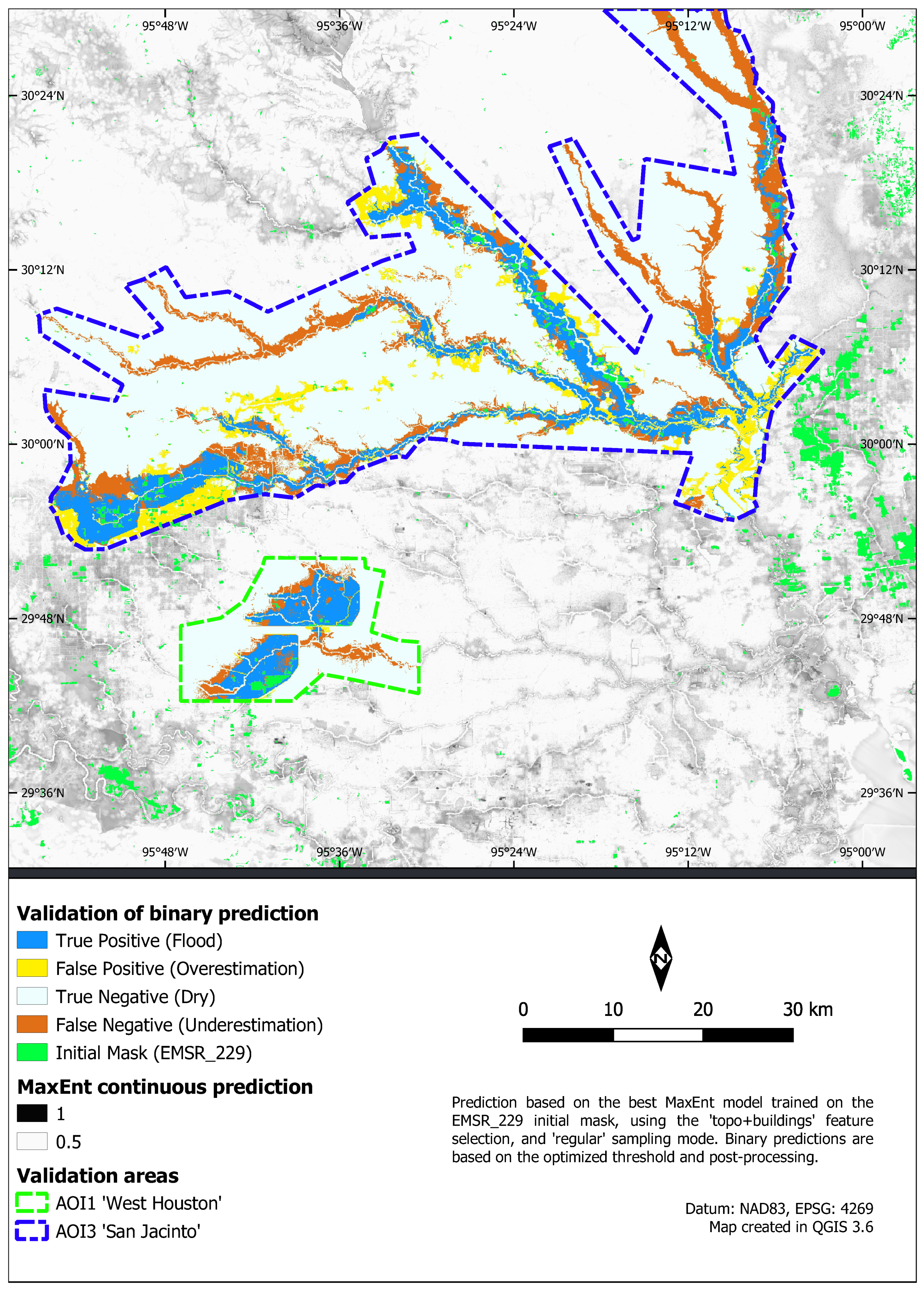
3.3. Spatial Comparison of Predicted Flood Extents

The large-scale comparison (Figure 7) visualizes the general behavior of an OCC model learned from the EMSR initial flood mask. The initial mask used for training (green) is primarily located outside the test areas. Some disagreement between the training mask and the validation mask is visible, especially in the west. The overestimation (yellow area) is explainable given the training data, which are learned as true extent. Note that the NOAA_labeled reference has been created by us, and we are accordingly confident about the quality, while the USGS_SJ mapping on the other hand is based on interpolated high water marks and could contain errors which we cannot further evaluate. Note also that the underestimation visible on the map (red) stems to large parts from the postprocessing, which removes predicted flood without spatial connection to the initial mask. This is especially obvious for the channel of the Buffalo Bayou, which is completely missing on the postprocessed version. The continuous prediction outside the validation areas shows that the model has indeed learned quite smooth and understandable patterns along the rivers. It is also obvious that the models correctly learned to exclude the permanent river channels.

An example model trained on DLR_BN (Figure 8) exhibits large fractions of correctly identified flooded vegetation and coarse coverage of the affected urban areas. Visually disturbing is the buffer around the channels that has been classified as non-flood, which is also seen on the initial mask. This is probably an artifact from training on flood masks instead of water masks. The area around these streams is covered by dense forest. Note that the previously shown EMSR_229 model performed better along these channels, presumably because it could learn the relationships of flooding along other streams, which are less obstructed by vegetation. The DLR_BN model performs much better on urban areas, though. There is underestimation visible along the Buffalo Bayou settlements, yet the affected urban areas in the north and south-west are captured quite well. These areas are colored mainly in yellow (overdetection) because the model did not restrict the predictions to the streets, which are visible as fine blue patterns, but the affected area seems reasonable. The overestimation along the western channel is not removed during postprocessing due to spatial connection with unluckily distributed noise on the initial mask. Even with the highest quality initial mask, DLR_CNN (Figure 9), water in the streets remains mostly undetected. Still, the extrapolation outside the training area, visible in dark colors, appears smooth and connected. Noise from the initial mask has been entirely eliminated. The land-water boundary appears quite sharp.

4. Discussion

4.1. Aim and Overall Success

The assessed satellite-based flood masks exhibit very low (EMSR_229) to moderate (DLR_BN, DLR_CNN) detection skill in vegetated and urban areas. This is to be expected, due to the various effects which constrain the information content of SAR images in these cases, that is, volume scattering, layover, oblique viewing geometries, and others. The specificity of all these products is very high, though, meaning that those areas, which are identified as flooded, indeed represent true flood. We therefore propose to treat such products as PU data. Our study demonstrates how these satellite-based flood masks can then be improved in vegetated and urban areas by an OCC procedure. A critical point for such studies is the reliability of the reference data. We present a performance evaluation on a precisely labeled aerial image, which is of higher quality than what is frequently used in other studies (e.g., [62,63]). For the larger scale, we use the extent in the San Jacinto river as published by the USGS, which is based on interpolated HWM and has been used as reference by [44].

According to the performance metrics, all initial flood masks can be considerably improved by the presented procedure. For the EMSR product, $\kappa$ over all classes rose from 0.06 to 0.76 in the best case with postprocessing, and from 0.00 to 0.25 in urban areas. The high quality initial masks, DLR_BN and DLR_CNN, have also been successfully enhanced up to about 0.2 points. Although the raw classification may at first lead to some overestimation far off the initial mask, the postprocessing improved the specificity as well as the visually perceived quality of the results, by suppressing uncorrelated errors of the initial SAR classification and our classification from topographic data. In a pluvial event, the formation of disconnected puddles is possible. The region-growing may delete such correctly predicted puddles from the classification. However, if the initial satellite mask contains a single pixel of that puddle, the area is kept. Whether or not to apply this postprocessing is therefore also a question of the quality of the initial mask. Overestimation after the postprocessing occurs mainly in places where the reference mask disagrees with the input mask, meaning either false positives in the input or false negatives in the reference data. For USGS_SJ, some uncertainty is to be expected. For NOAA_labeled, minor differences might be induced by the different acquisition times of the aerial and satellite images. The models were explicitly trained on flood masks. For many applications it might be more suitable to generate water masks, which include the permanent water. This should also solve the visible underdetection along the streams in the DLR_BN models. We refer to extrapolation as growing areas of flood detected on the initial datasets. Spatial transfer (e.g., DLR_BN to USGS_SJ) did not work well. A local approach is necessary, because event characteristics differ spatially. Although some extrapolation outside the extent of the initial mask is possible, the predictions far off the original extent, and especially in different river basins, are therefore deemed unreliable (note the difference here is between undetected flood on the original extent of the satellite image, and areas outside the satellite image). Whether the area in between two or more satellite images could be modelled by this approach has not been investigated, but could be an interesting question to try in future studies.

4.2. Features and Algorithms

Our analysis was based on features that have commonly been suggested in the literature for the purpose of flood susceptibility mapping [29,30,31,32,64], like HAND, TWI, distance to streams and descriptors of the local topographic situation. The skill of the PN benchmark models suggests that these features are indeed useful, also in urban and vegetated areas, given a representative training set. In addition we tested whether rainfall data and distance to buildings help to improve the models. The rainfall sum for hurricane Harvey had very little spatial variance over the Houston area, therefore it is rather unsurprising that it does not lead to an improvement here. We hesitate to draw a general conclusion from this result, as the effect may be different for an event with more heterogeneous rainfall distribution. The results of our investigation did neither show clear improvements from using distance to buildings as a feature, nor from drawing more training samples from urban areas, when learning from the DLR_BN initial mask. However, the skill of the models learned from EMSR_229 did improve slightly, and the transfer skill of models learned from DLR_CNN to AOI1 did improve strongly, when including the distance to buildings. The sampling further seems to have at least a small effect on the skill on urban areas for the EMSR_229 models. A possible explanation is that DLR_BN already covers significant parts of urban and non-urban areas alike, while DLR_CNN covers primarily urban flood, and EMSR_229 almost exclusively non-urban flood. Therefore, the distance to buildings might be more useful in these models to describe how feature distributions of flooded areas differ closer to and further away from the city, respectively. Since the results do not indicate any negative effect of including the distance to buildings, we suggest to include it when available. To further improve the feature engineering, automating this step via deep learning might be an idea worth investigating in future studies. Especially local context features, as generated by a CNN, have been successful in improving various land cover classifications, including detection of water [65,66].

Both tested OCC algorithms, BSVM and MaxEnt, performed similarly well in the overall statistics. BSVM exhibits a closer fit to the training data, and is less affected by feature selection and sampling. Ng & Jordan [67] state that discriminative algorithms often perform better than generative algorithms for complex classification problems. This might partially explain why BSVM in most cases performs better than MaxEnt in detecting urban flooding. However, explaining this finding remains speculative to a certain extent. The best models on AOI1 and AOI2 also came close to the PN benchmark, but there is still a significant margin which indicates potential for improvement. While we assume that our positive training labels are mostly correct, there will for sure be some violation of this assumption. BSVM can theoretically handle this problem to a certain extent, because outliers in the positive training samples will be classified as negative if they are so far in the “negative realm” that the biased penalty term is overruled. MaxEnt assumes positive samples to be clean from errors [53], so a preprocessing of the initial masks might be an option to consider. Instead of performing classification in one step, it is also possible to iteratively single out the reliable negatives [41]. As the amount of available training samples in our task is relatively high, we did not implement such an iterative refinement, but rather relied of the effectiveness of data. The effect of training label distribution is debated and difficult to estimate without doing systematic tests for each dataset, as the naturally occurring class distribution—even in cases where there is such a distribution – is often not the most appropriate [68]. Besides this, also other PU algorithms are available in the literature, for example, [69,70]. If a validity layer for the initial flood mask is available, an alternative approach would be to train any regular PN classifier on the valid areas. Hydrodynamic simulations are able to model flooding in vegetated and urban areas as well, for example, Wing et al. [44] for the event in question. A drawback of our presented approach in comparison to a physical model is that the machine learning models do not account for hydrodynamic effects, or in general a closed water balance (no more water predicted than available). However, we argue that a hydrodynamic simulation could make use of the improved flood masks from our approach via data assimilation.

4.3. Threshold Selection

As this paper presents a novel approach, rather than a particular classification, we provide the threshold-independent score $AU{C}_{PN}$, further performance metrics at ${\theta }_{Opt}$, and the loss $\Delta \kappa$ when resorting to ${\theta }_{Default}$. We are fully aware that optimal threshold selection in the absence of PN reference data is tricky. By which metric the user optimizes the threshold selection will depend on the application case, that is, how much sensitivity or specificity is required. Maximum $\kappa$ may not be the desired quantity. Mack et al. [41] further suggested a manual approach (i.e., not automated) to derive a maximum a-posteriori threshold from a Gaussian mixture model analysis of the posterior density of the continuous prediction. However, that procedure is based on the assumptions that the posterior can be described by a combination of Gaussians, and that the component with the highest mean value is equal to the positive class, while all other components belong to the negative class. Another assumption in their approach is that the classes do not overlap at a specified point used to estimate the prior probabilities. These assumptions are certainly violated for some of our models, and this approach is not feasible in the context of this paper, as we compare many models to get an idea of the upper bound of performance of our procedure. MaxEnt also provides a different form of output, called the cumulative format, which allows setting a threshold based on the accepted omission rate [71]. Depending on the application, this may be a more desirable way of threshold selection. In cases where the training data is representative, the most straightforward approach is to use the default threshold or to optimize a PU performance metric of choice on the training data. For the benchmark models, training and application data were drawn from the same underlying distribution, and in that case the skill at ${\theta }_{Default}$ and ${\theta }_{Opt}$ is almost identical. This proves that the procedure is in principle able to obtain very good results, given a representative training set. In the application using satellite-based flood masks, a bias in the feature distributions of the positive training samples is to be expected, as we know that the areas detected from satellite imagery are not entirely representative of the true flood extent. Elith et al. [53] claim that PU models are even stronger affected by sample bias than PN models, because sample bias affects both positive and negative records in the PN case, but only the positive samples in the PU case. In our case, this “sample bias” corresponds to the representativeness of the initial flood mask. This leads us to assume that including additional positive class examples from within the urban area could make the positive training data more representative, and thereby improve the performance of the PU models at ${\theta }_{Default}$. Such data could potentially be taken from sources such as social media content or street camera footage, which is only punctually available but provides data from within the city center.

5. Conclusions

We presented an extrapolation technique for satellite-based flood masks to unobservable areas, by using OCC algorithms. Especially vegetated and urban areas still pose a challenge to currently available remote sensing products, the latter of which are of major importance for impact estimation. The quality of the initial EMSR_229 mask was found to be poor, detecting almost exclusively open water. Although it does exhibit very high specificity, a map with extreme specificity but very low sensitivity is trivial (only few easy-to-find spots detected) and of limited practical value. As long as the spatial validity of satellite-based flood masks is not clearly communicated, for example, by a separate validity layer, we suggest treating them as positive and unlabeled in this context. OCC is then the adequate tool, avoiding to explicitly train unobservable areas as “non-flooded”. Using supervised machine learning for extrapolation is straightforward once using an OCC, as the necessary positive labels for training are readily available from the initial mask. Our procedure allows for predicting a continuous score of how likely flood is to be expected per pixel, given the original mapping and the used features. A threshold can then be applied to derive a binary classification, and a subsequent region-growing raises the specificity of the extrapolation. From the user’s perspective, the presented method is relatively simple to use, as the entire initial mask can be processed without the need to exclude any areas from sampling. The most important features can already be generated from a DEM and stream locations (which can also be derived from a DEM if necessary). Distance to building footprints and gridded rainfall data did not consistently improve the results, although positive effects were observed for some models.

We conclude that all three of the tested satellite-based products have been improved to a certain extent. The absolute quality of the extrapolation, as well as the suitability of the default threshold in application, hinges on the representativeness of the initial mask. The features used in this study are not sufficient for a full separation of flooded and dry locations, but a model trained on representative training data still achieves high performance ($AU{C}_{PN}$ 0.91-0.98 in the benchmark case, 0.94 for the best PU model). The method in its current form may be useful for statistical applications on a scale where satellite imagery is utilized. It is not yet fit for analysis of individual streets, although the results with high quality input seem promising. Potential application of the presented method is not limited to masks from SAR data—it could also be used to fill holes from clouds in masks from optical data, or tested for social media derived extents. In particular, we see potential for future studies in the fusion of satellite-based flood masks with spottily mapped flood locations within a city center, for example, by social media or street camera footage. Such a fused dataset is expected to provide more representative coverage in feature space, which should lead to a more reliable default threshold. The presented approach could be tested in this direction with the aim of deriving more reliable flood extents in vegetated and urban areas.

References

1. Hostache, R.; Chini, M.; Giustarini, L.; Neal, J.; Kavetski, D.; Wood, M.; Corato, G.; Pelich, R.M.; Matgen, P. Near-Real-Time Assimilation of SAR-Derived Flood Maps for Improving Flood Forecasts. Water Resour. Res. 2018, 54, 5516–5535. [Google Scholar] [CrossRef]
2. Mason, D.; Speck, R.; Devereux, B.; Schumann, G.P.; Neal, J.; Bates, P. Flood Detection in Urban Areas Using TerraSAR-X. IEEE Trans. Geosci. Remote Sens. 2010, 48, 882–894. [Google Scholar] [CrossRef] [Green Version]
3. Pulvirenti, L.; Chini, M.; Pierdicca, N.; Boni, G. Use of SAR Data for Detecting Floodwater in Urban and Agricultural Areas: The Role of the Interferometric Coherence. IEEE Trans. Geosci. Remote Sens. 2016, 54, 1532–1544. [Google Scholar] [CrossRef]
4. Sieg, T.; Vogel, K.; Merz, B.; Kreibich, H. Seamless Estimation of Hydrometeorological Risk Across Spatial Scales. Earth’s Future 2019. [Google Scholar] [CrossRef] [Green Version]
5. Henderson, F.M.; Lewis, A.J. Radar detection of wetland ecosystems: A review. Int. J. Remote Sens. 2008, 29, 5809–5835. [Google Scholar] [CrossRef]
6. Plank, S.; Jüssi, M.; Martinis, S.; Twele, A. Mapping of flooded vegetation by means of polarimetric Sentinel-1 and ALOS-2/PALSAR-2 imagery. Int. J. Remote Sens. 2017, 38, 3831–3850. [Google Scholar] [CrossRef]
7. Zwenzner, H.; Voigt, S. Improved estimation of flood parameters by combining space based SAR data with very high resolution digital elevation data. Hydrol. Earth Syst. Sci. Discuss. 2008, 5, 2951–2973. [Google Scholar] [CrossRef]
8. Cian, F.; Marconcini, M.; Ceccato, P.; Giupponi, C. Flood depth estimation by means of high-resolution SAR images and lidar data. Nat. Hazards Earth Syst. Sci. 2018, 18, 3063–3084. [Google Scholar] [CrossRef] [Green Version]
9. Cohen, S.; Brakenridge, G.R.; Kettner, A.; Bates, B.; Nelson, J.; McDonald, R.; Huang, Y.F.; Munasinghe, D.; Zhang, J. Estimating Floodwater Depths from Flood Inundation Maps and Topography. JAWRA J. Am. Water Resour. Assoc. 2017, 54, 847–858. [Google Scholar] [CrossRef]
10. Matgen, P.; Giustarini, L.; Chini, M.; Hostache, R.; Wood, M.; Schlaffer, S. Creating a water depth map from SAR flood extent and topography data. In Proceedings of the 2016 IEEE International Geoscience and Remote Sensing Symposium (IGARSS), Beijing, China, 10–16 July 2016. [Google Scholar] [CrossRef]
11. Schumann, G.; Pappenberger, F.; Matgen, P. Estimating uncertainty associated with water stages from a single SAR image. Adv. Water Resour. 2008, 31, 1038–1047. [Google Scholar] [CrossRef]
12. Stephens, E.; Bates, P.; Freer, J.; Mason, D. The impact of uncertainty in satellite data on the assessment of flood inundation models. J. Hydrol. 2012, 414–415, 162–173. [Google Scholar] [CrossRef] [Green Version]
13. Giustarini, L.; Vernieuwe, H.; Verwaeren, J.; Chini, M.; Hostache, R.; Matgen, P.; Verhoest, N.; Baets, B.D. Accounting for image uncertainty in SAR-based flood mapping. Int. J. Appl. Earth Obs. Geoinf. 2015, 34, 70–77. [Google Scholar] [CrossRef]
14. Martinis, S.; Rieke, C. Backscatter Analysis Using Multi-Temporal and Multi-Frequency SAR Data in the Context of Flood Mapping at River Saale, Germany. Remote Sens. 2015, 7, 7732–7752. [Google Scholar] [CrossRef] [Green Version]
15. Martinis, S.; Twele, A.; Voigt, S. Towards operational near real-time flood detection using a split-based automatic thresholding procedure on high resolution TerraSAR-X data. Nat. Hazards Earth Syst. Sci. 2009, 9, 303–314. [Google Scholar] [CrossRef]
16. Horritt, M.S.; Mason, D.C.; Luckman, A.J. Flood boundary delineation from Synthetic Aperture Radar imagery using a statistical active contour model. Int. J. Remote Sens. 2001, 22, 2489–2507. [Google Scholar] [CrossRef]
17. Pulvirenti, L.; Pierdicca, N.; Chini, M.; Guerriero, L. An algorithm for operational flood mapping from Synthetic Aperture Radar (SAR) data using fuzzy logic. Nat. Hazards Earth Syst. Sci. 2011, 11, 529–540. [Google Scholar] [CrossRef] [Green Version]
18. Twele, A.; Cao, W.; Plank, S.; Martinis, S. Sentinel-1-based flood mapping: A fully automated processing chain. Int. J. Remote Sens. 2016, 37, 2990–3004. [Google Scholar] [CrossRef]
19. Schlaffer, S.; Matgen, P.; Hollaus, M.; Wagner, W. Flood detection from multi-temporal SAR data using harmonic analysis and change detection. Int. J. Appl. Earth Obs. Geoinf. 2015, 38, 15–24. [Google Scholar] [CrossRef]
20. Li, Y.; Martinis, S.; Wieland, M.; Schlaffer, S.; Natsuaki, R. Urban Flood Mapping Using SAR Intensity and Interferometric Coherence via Bayesian Network Fusion. Remote Sens. 2019, 11, 2231. [Google Scholar] [CrossRef] [Green Version]
21. Li, Y.; Martinis, S.; Wieland, M. Urban flood mapping with an active self-learning convolutional neural network based on TerraSAR-X intensity and interferometric coherence. ISPRS J. Photogramm. Remote Sens. 2019, 152, 178–191. [Google Scholar] [CrossRef]
22. Bonafilia, D.; Tellman, B.; Anderson, T.; Issenberg, E. Sen1Floods11: A georeferenced dataset to train and test deep learning flood algorithms for Sentinel-1. In Proceedings of the 2020 IEEE/CVF Conference on Computer Vision and Pattern Recognition Workshops (CVPRW), Seattle, WA, USA, 14–19 June 2020. [Google Scholar] [CrossRef]
23. Chini, M.; Pelich, R.; Pulvirenti, L.; Pierdicca, N.; Hostache, R.; Matgen, P. Sentinel-1 InSAR Coherence to Detect Floodwater in Urban Areas: Houston and Hurricane Harvey as A Test Case. Remote Sens. 2019, 11, 107. [Google Scholar] [CrossRef] [Green Version]
24. Wieland, M.; Martinis, S. A Modular Processing Chain for Automated Flood Monitoring from Multi-Spectral Satellite Data. Remote Sens. 2019, 11, 2330. [Google Scholar] [CrossRef] [Green Version]
25. Mason, D.; Schumann, G.P.; Neal, J.; Garcia-Pintado, J.; Bates, P. Automatic near real-time selection of flood water levels from high resolution Synthetic Aperture Radar images for assimilation into hydraulic models: A case study. Remote Sens. Environ. 2012, 124, 705–716. [Google Scholar] [CrossRef] [Green Version]
26. Huang, C.; Nguyen, B.D.; Zhang, S.; Cao, S.; Wagner, W. A Comparison of Terrain Indices toward Their Ability in Assisting Surface Water Mapping from Sentinel-1 Data. ISPRS Int. J. Geo-Inf. 2017, 6, 140. [Google Scholar] [CrossRef] [Green Version]
27. Scotti, V.; Giannini, M.; Cioffi, F. Enhanced flood mapping using synthetic aperture radar (SAR) images, hydraulic modelling, and social media: A case study of Hurricane Harvey (Houston, TX). J. Flood Risk Manag. 2020. [Google Scholar] [CrossRef]
28. Martinis, S. A Sentinel-1 Times Series-Based Exclusion Layer for Improved Flood Mapping in Arid Areas. In Proceedings of the IGARSS 2018—2018 IEEE International Geoscience and Remote Sensing Symposium, Valencia, Spain, 22–27 July 2018. [Google Scholar] [CrossRef]
29. Samela, C.; Troy, T.J.; Manfreda, S. Geomorphic classifiers for flood-prone areas delineation for data-scarce environments. Adv. Water Resour. 2017, 102, 13–28. [Google Scholar] [CrossRef]
30. Chapi, K.; Singh, V.P.; Shirzadi, A.; Shahabi, H.; Bui, D.T.; Pham, B.T.; Khosravi, K. A novel hybrid artificial intelligence approach for flood susceptibility assessment. Environ. Model. Softw. 2017, 95, 229–245. [Google Scholar] [CrossRef]
31. Tehrany, M.S.; Kumar, L.; Jebur, M.N.; Shabani, F. Evaluating the application of the statistical index method in flood susceptibility mapping and its comparison with frequency ratio and logistic regression methods. Geomat. Nat. Hazards Risk 2018, 10, 79–101. [Google Scholar] [CrossRef]
32. Kelleher, C.; McPhillips, L. Exploring the application of topographic indices in urban areas as indicators of pluvial flooding locations. Hydrol. Process. 2019, 34, 780–794. [Google Scholar] [CrossRef]
33. Mukherjee, F.; Singh, D. Detecting flood prone areas in Harris County: A GIS based analysis. GeoJournal 2019, 85, 647–663. [Google Scholar] [CrossRef]
34. Rennó, C.D.; Nobre, A.D.; Cuartas, L.A.; Soares, J.V.; Hodnett, M.G.; Tomasella, J.; Waterloo, M.J. HAND, a new terrain descriptor using SRTM-DEM: Mapping terra-firme rainforest environments in Amazonia. Remote Sens. Environ. 2008, 112, 3469–3481. [Google Scholar] [CrossRef]
35. Quinn, P.; Beven, K.; Chevallier, P.; Planchon, O. The prediction of hillslope flow paths for distributed hydrological modelling using digital terrain models. Hydrol. Process. 1991, 5, 59–79. [Google Scholar] [CrossRef]
36. Phillips, S.J.; Anderson, R.P.; Schapire, R.E. Maximum entropy modeling of species geographic distributions. Ecol. Model. 2006, 190, 231–259. [Google Scholar] [CrossRef] [Green Version]
37. Mack, B.; Roscher, R.; Stenzel, S.; Feilhauer, H.; Schmidtlein, S.; Waske, B. Mapping raised bogs with an iterative one-class classification approach. ISPRS J. Photogramm. Remote Sens. 2016, 120, 53–64. [Google Scholar] [CrossRef]
38. Piiroinen, R.; Fassnacht, F.E.; Heiskanen, J.; Maeda, E.; Mack, B.; Pellikka, P. Invasive tree species detection in the Eastern Arc Mountains biodiversity hotspot using one class classification. Remote Sens. Environ. 2018, 218, 119–131. [Google Scholar] [CrossRef]
39. Ortiz, S.; Breidenbach, J.; Kändler, G. Early Detection of Bark Beetle Green Attack Using TerraSAR-X and RapidEye Data. Remote Sens. 2013, 5, 1912–1931. [Google Scholar] [CrossRef] [Green Version]
40. Jozani, H.J.; Thiel, M.; Abdel-Rahman, E.M.; Richard, K.; Landmann, T.; Subramanian, S.; Hahn, M. Investigation of Maize Lethal Necrosis (MLN) severity and cropping systems mapping in agro-ecological maize systems in Bomet, Kenya utilizing RapidEye and Landsat-8 Imagery. Geol. Ecol. Landsc. 2020, 1–16. [Google Scholar] [CrossRef]
41. Mack, B.; Waske, B. In-depth comparisons of MaxEnt, biased SVM and one-class SVM for one-class classification of remote sensing data. Remote Sens. Lett. 2016, 8, 290–299. [Google Scholar] [CrossRef]
42. Liu, B.; Dai, Y.; Li, X.; Lee, W.; Yu, P. Building text classifiers using positive and unlabeled examples. In Proceedings of the Third IEEE International Conference on Data Mining, Melbourne, FL, USA, 22 November 2003. [Google Scholar] [CrossRef]
43. NHC. Costliest U.S. Tropical Cyclones Tables Updated; Technical Report; National Hurricane Center: Miami, FL, USA, 2018.
44. Wing, O.E.; Sampson, C.C.; Bates, P.D.; Quinn, N.; Smith, A.M.; Neal, J.C. A flood inundation forecast of Hurricane Harvey using a continental-scale 2D hydrodynamic model. J. Hydrol. X 2019, 4, 100039. [Google Scholar] [CrossRef]
45. Lindner, J.; Fitzgerald, S. Hurricane Harvey—Storm and Flood Information; Technical Report; Harris County Flood Control District (HCFCD): Houston, TX, USA, 2018. [Google Scholar]
46. HCFCD. Hurricane Harvey: Impact and Response in Harris County; Technical Report; Harris County Flood Control District: Houston, TX, USA, 2018. [Google Scholar]
47. Watson, K.M.; Harwell, G.R.; Wallace, D.S.; Welborn, T.L.; Stengel, V.G.; McDowell, J.S. Characterization of Peak Streamflows and Flood Inundation of Selected Areas in Southeastern Texas and southwestern Louisiana from the August and September 2017 Flood Resulting from Hurricane Harvey; U.S. Geological Survey: Austin, TX, USA, 2018. [CrossRef]
48. Arundel, S.; Phillips, L.; Lowe, A.; Bobinmyer, J.; Mantey, K.; Dunn, C.; Constance, E.; Usery, E. PreparingThe National Mapfor the 3D Elevation Program—Products, process and research. Cartogr. Geogr. Inf. Sci. 2015, 42, 40–53. [Google Scholar] [CrossRef]
49. Reu, J.D.; Bourgeois, J.; Bats, M.; Zwertvaegher, A.; Gelorini, V.; Smedt, P.D.; Chu, W.; Antrop, M.; Maeyer, P.D.; Finke, P.; et al. Application of the topographic position index to heterogeneous landscapes. Geomorphology 2013, 186, 39–49. [Google Scholar] [CrossRef]
50. Evans, J.S. spatialEco. 2021. R Package Version 1.3-6. Available online: https://github.com/jeffreyevans/spatialEco (accessed on 21 May 2021).
51. Jaynes, E.T. Information Theory and Statistical Mechanics. Phys. Rev. 1957, 106, 620–630. [Google Scholar] [CrossRef]
52. Phillips, S.J.; Anderson, R.P.; Dudík, M.; Schapire, R.E.; Blair, M.E. Opening the black box: An open-source release of Maxent. Ecography 2017, 40, 887–893. [Google Scholar] [CrossRef]
53. Elith, J.; Phillips, S.J.; Hastie, T.; Dudík, M.; Chee, Y.E.; Yates, C.J. A statistical explanation of MaxEnt for ecologists. Divers. Distrib. 2010, 17, 43–57. [Google Scholar] [CrossRef]
54. Guillera-Arroita, G.; Lahoz-Monfort, J.J.; Elith, J. Maxent is not a presence-absence method: A comment on Thibaudet al. Methods Ecol. Evol. 2014, 5, 1192–1197. [Google Scholar] [CrossRef]
55. Merow, C.; Smith, M.J.; Silander, J.A. A practical guide to MaxEnt for modeling species’ distributions: What it does, and why inputs and settings matter. Ecography 2013, 36, 1058–1069. [Google Scholar] [CrossRef]
56. Lowekamp, B.C.; Chen, D.T.; Ibáñez, L.; Blezek, D. The Design of SimpleITK. Front. Neuroinformatics 2013, 7. [Google Scholar] [CrossRef] [PubMed] [Green Version]
57. Lee, W.S.; Liu, B. Learning with Positive and Unlabeled Examples Using Weighted Logistic Regression. In Proceedings of the Twentieth International Conference on Machine Learning (ICML-2003), Washington, DC, USA, 21–24 August 2003; Volume 20, pp. 448–455. [Google Scholar]
58. Mack, B.; Roscher, R.; Waske, B. Can I Trust My One-Class Classification? Remote Sens. 2014, 6, 8779–8802. [Google Scholar] [CrossRef] [Green Version]
59. Hanley, J.A.; McNeil, B.J. The meaning and use of the area under a receiver operating characteristic (ROC) curve. Radiology 1982, 143, 29–36. [Google Scholar] [CrossRef] [Green Version]
60. Fawcett, T. An introduction to ROC analysis. Pattern Recognit. Lett. 2006, 27, 861–874. [Google Scholar] [CrossRef]
61. Cohen, J. A Coefficient of Agreement for Nominal Scales. Educ. Psychol. Meas. 1960, 20, 37–46. [Google Scholar] [CrossRef]
62. Giustarini, L.; Hostache, R.; Matgen, P.; Schumann, G.J.P.; Bates, P.D.; Mason, D.C. A Change Detection Approach to Flood Mapping in Urban Areas Using TerraSAR-X. IEEE Trans. Geosci. Remote Sens. 2013, 51, 2417–2430. [Google Scholar] [CrossRef] [Green Version]
63. Matgen, P.; Hostache, R.; Schumann, G.; Pfister, L.; Hoffmann, L.; Savenije, H. Towards an automated SAR-based flood monitoring system: Lessons learned from two case studies. Phys. Chem. Earth Parts A/B/C 2011, 36, 241–252. [Google Scholar] [CrossRef]
64. Jalayer, F.; Risi, R.D.; Paola, F.D.; Giugni, M.; Manfredi, G.; Gasparini, P.; Topa, M.E.; Yonas, N.; Yeshitela, K.; Nebebe, A.; et al. Probabilistic GIS-based method for delineation of urban flooding risk hotspots. Nat. Hazards 2014. [Google Scholar] [CrossRef]
65. Yu, L.; Wang, Z.; Tian, S.; Ye, F.; Ding, J.; Kong, J. Convolutional Neural Networks for Water Body Extraction from Landsat Imagery. Int. J. Comput. Intell. Appl. 2017, 16, 1750001. [Google Scholar] [CrossRef]
66. Wu, G.; Guo, Y.; Song, X.; Guo, Z.; Zhang, H.; Shi, X.; Shibasaki, R.; Shao, X. A Stacked Fully Convolutional Networks with Feature Alignment Framework for Multi-Label Land-cover Segmentation. Remote Sens. 2019, 11, 1051. [Google Scholar] [CrossRef] [Green Version]
67. Ng, A.Y.; Jordan, M.I. On Discriminative vs. Generative Classifiers: A comparison of logistic regression and naive Bayes. In Advances in Neural Information Processing Systems 14; Dietterich, T.G., Becker, S., Ghahramani, Z., Eds.; MIT Press: Cambridge, MA, USA, 2002; pp. 841–848. [Google Scholar]
68. Weiss, G.M.; Provost, F. The effect of class distribution on classifier learning: An empirical study. Rutgers Univ. 2001. [Google Scholar] [CrossRef]
69. Li, W.; Guo, Q.; Elkan, C. A Positive and Unlabeled Learning Algorithm for One-Class Classification of Remote-Sensing Data. IEEE Trans. Geosci. Remote Sens. 2011, 49, 717–725. [Google Scholar] [CrossRef]
70. Ruff, L.; Vandermeulen, R.; Goernitz, N.; Deecke, L.; Siddiqui, S.A.; Binder, A.; Müller, E.; Kloft, M. Deep One-Class Classification. In Proceedings of Machine Learning Research, Proceedings of the 35th International Conference on Machine Learning, PMLR, Stockholm, Sweden, 10–15 July 2018; Dy, J., Krause, A., Eds.; Rutgers University: New Brunswick, NJ, USA, 2018; Volume 80, pp. 4393–4402. [Google Scholar]
71. Phillips, S.J.; Dudík, M. Modeling of species distributions with Maxent: New extensions and a comprehensive evaluation. Ecography 2008, 31, 161–175. [Google Scholar] [CrossRef]
Figure 1. Overview map including the three AOIs, the USGS interpolation of high water marks (HWM), and the manually labeled aerial image from 30 August 2017. (A) Full extent. (B) West Houston extent. The large vegetated areas are the Addicks reservoir (north) and Barker reservoir (south). (C) Buffalo Bayou extent. Note the detailed mapping of streets. EMSR_229 covers the entire area depicted on subplot A, while DLR_BN is available for AOI1 and DLR_CNN for AOI2.
Remotesensing 13 02042 g001
Figure 2. PU vs PN performance of all candidate models during the grid search for selected setups. Each point represents a model trained on the same data, but with different parameters. A U C P U is given as the mean of a 5-fold cross validation, A U C P N is a single score computed on an independent test set of the reference data on the corresponding AOI. (A) shows a BSVM trained on EMSR_229 and using USGS_SJ as test set. (B) shows a BSVM trained on DLR_BN and using NOAA_labeled as test set. (C) shows MaxEnt models trained on EMSR_229 and using USGS_SJ as test set. The green dot signals the selected model by the criterion of maximum A U C P U , which has been the basis of model selection for this study.
Remotesensing 13 02042 g002
Figure 3. Flowchart of the presented procedure.
Remotesensing 13 02042 g003
Figure 4. κ score on validation data at θ O p t without postprocessing. The green triangle denotes the skill of the original product (initial mask) if the product exists on that AOI. Each point represents a model with different setup. BSVM and MaxEnt have been trained with identical data.
Remotesensing 13 02042 g004
Figure 5. Difference of default and optimal threshold. Δ θ denotes the difference in the threshold value and Δ κ the respective difference in skill.
Remotesensing 13 02042 g005
Figure 6. Overall effect of postprocessing on κ , sensitivity and specificity at θ O p t . The range of the boxplots includes both BSVM and MaxEnt models to visualize the general trend. Empty boxes indicate that postprocessing is not possible because the initial mask does not exist on that extent. Note that EMSR_229 is theoretically defined on AOI2, but there was no flood detected in that area, therefore the region-growing would remove all predictions there.
Remotesensing 13 02042 g006
Figure 7. Example of the spatial prediction of a MaxEnt model learned from EMSR_229.
Remotesensing 13 02042 g007
Figure 8. Example of the spatial prediction of a BSVM model learned from DLR_BN.
Remotesensing 13 02042 g008
Figure 9. Example of the spatial prediction of a BSVM model learned from DLR_CBN. Water in the streets is not detected, although some fine patters are visible in the continuous prediction.
Remotesensing 13 02042 g009