A Strategy of Parallel Seed-Based Image Segmentation Algorithms for Handling Massive Image Tiles over the Spark Platform

Abstract

The volume of remote sensing images continues to grow as image sources become more diversified and with increasing spatial and spectral resolution. The handling of such large-volume datasets, which exceed available CPU memory, in a timely and efficient manner is becoming a challenge for single machines. The distributed cluster provides an effective solution with strong calculation power. There has been an increasing number of big data technologies that have been adopted to deal with large images using mature parallel technology. However, since most commercial big data platforms are not specifically developed for the remote sensing field, two main issues exist in processing large images with big data platforms using a distributed cluster. On the one hand, the quantities and categories of official algorithms used to process remote sensing images in big data platforms are limited compared to large amounts of sequential algorithms. On the other hand, the sequential algorithms employed directly to process large images in parallel over a distributed cluster may lead to incomplete objects in the tile edges and the generation of large communication volumes at the shuffle stage. It is, therefore, necessary to explore the distributed strategy and adapt the sequential algorithms over the distributed cluster. In this research, we employed two seed-based image segmentation algorithms to construct a distributed strategy based on the Spark platform. The proposed strategy focuses on modifying the incomplete objects by processing border areas and reducing the communication volume to a reasonable size by limiting the auxiliary bands and the buffer size to a small range during the shuffle stage. We calculated the F-measure and execution time to evaluate the accuracy and execution efficiency. The statistical data reveal that both segmentation algorithms maintained high accuracy, as achieved in the reference image segmented in the sequential way. Moreover, generally the strategy took less execution time compared to significantly larger auxiliary bands and buffer sizes. The proposed strategy can modify incomplete objects, with execution time being twice as fast as the strategies that do not employ communication volume reduction in the distributed cluster.

1. Introduction

The volume of remote sensing images has been increasing exponentially over the last two decades. The number of earth observation satellites is growing rapidly, which will generate increasingly larger amounts of high-resolution images and will allow more detailed observation of the earth’s surface, with higher temporal and spatial resolution [1,2]. Such progress is due mainly to advances in sensor technologies and reductions in the costs to produce and launch satellites [3,4]. As a result, the processing of tremendously large images is becoming a challenge for end users [5], as the high spatial resolution images increase not only the richness but also the complexity of the information [6]. For example, mining knowledge from the Landsat image archives over more than 40 years has become an intractable issue for both manual and automatic processing capabilities [7,8]. Hence, there will be an increased demand for highly efficient image processing technologies capable of handling very large remote sensing images [9,10].

To overcome the above issues, big data platforms, such as the Hadoop platform [11] and the Spark platform [12], are imported to process the large remote sensing images over a distributed cluster [13]. As the big data platforms are not designed specifically for processing remote sensing images, the number and types of the official algorithms used in big data platforms are limited compared to the large amounts of sequential algorithms. In order to process large images efficiently with numerous traditional algorithms, such as object-based segmentation methods and graph-based methods [14,15], it is essential to integrate sequential algorithms into the big data platforms. The big data platforms provide the capability to organize and process large arbitrary datasets based on operations such as extraction, transformation, and loading [16]. With big data platforms, the sequential pixel-based and object-based algorithms may perform the corresponding procedures over the distributed cluster, with similar results to those implemented in a single machine. Although the big data platforms and sequential algorithms have matured recently, it remains challenging to apply sequential algorithms directly to big data platforms over a distributed cluster. To deal with this issue, distributed strategies have emerged and are used to adapt the sequential algorithms, which are suitable over the distributed cluster, to acquire the desired results. To the best of our knowledge, most research studies on distributed strategies in image processing have concentrated on specific algorithms [17]. Therefore, developing the distributed strategies to accommodate more sequential image processing algorithms in big data platforms is one of the practical solutions to take advantage of both big data platforms and traditional sequential image processing algorithms.

The distributed strategies for the various image processing algorithms may present different issues and challenges, although the basic workflows for big data platforms are similar. As described in many studies, the large image is first decomposed into multiple tiles, then the tiles are processed with specific algorithms simultaneously in big data platforms [4,18]. The pixel-based methods may be applied directly to tiles without modification, such as the normalized difference vegetation index. The object-based image analysis (OBIA) [19,20] methods tend to lead to incomplete object problems generated at the tile edges (artifacts) of the results if they are employed directly to process the tiles, as the divisions of the tiles are purely mechanical based on the tile size parameters. These issues encountered in OBIA deserve further research, because the OBIA synthesizes the spectral, morphological, texture, and shape information derived from the image objects [21,22]. Moreover, the OBIA has been widely employed to recognize and analyze the landscape patterns in multiple sequential applications [23,24]. Image segmentation is one of the critical operations of the OBIA to derive image objects [25,26]. Hence, in this paper, the image segmentation algorithms are used as a case study to construct the distributed strategy.

In recent years, a number of research groups have channeled their efforts into developing distributed strategies for large images with sequential image segmentation algorithms [27,28,29]. Michel, Youssefi [6], for example, presented a stable mean-shift segmentation algorithm to provide artifact-free results. Lassalle, Inglada [30] proposed a solution for a region-merging algorithm to ensure equivalent results. Both of the aforementioned works were conducted based on a scalable tile-based framework to produce similar results with respect to the sequential results. Wang, Chen [18] proposed a distributed strategy for both multi-resolution and graph-based segmentation to modify incomplete objects via several recalculations. However, the studies referred to above only discuss the accuracy between the parallel and the sequential results, while the execution efficiency of the strategies is ignored. Happ, da Costa [4] presented a distributed strategy for region-growing to tackle the artifacts that occur in the tile borders according to the specific indexing mechanism and hierarchical stitching method. Ye, Liu [31] reported on a raster dataset cleaning and reconstitution multi-grid architecture for remote sensing monitoring of vegetation dryness by using several operations on different types of datasets. Gotz, Cavallaro [32] proposed a hybrid algorithm for the parallel computation of two particular trees. The flooding-based algorithm was employed for the node-local computation, while the tuple-based merging scheme was adopted to merge the partial images into a globally correct view. Gu, Han [33] developed a parallel multi-scale segmentation method by combining the minimum spanning tree and the minimum heterogeneity rule, according to the message passing interface parallel technology. Huang, Chen [34] investigated a parallel mean shift algorithm based on a task-scheduling method with a message-passing interface and an OpenCL (computing language) model. Gazagnes and Wilkinson [35] presented a distributed connected component filtering and analysis method by adapting the flooding techniques to build the components trees and by implementing the merging approach to extend the computation scale. This research extended the dynamic range from 2D to 3D or higher dynamic range data sets. The focus was more on the evaluation of the execution efficiency, and the accuracy comparisons were insufficient for the six studies highlighted above. Derksen, Inglada [36] described a tile-based method for the modified simple linear iterative clustering (SLIC) to overcome the segmentation errors that appear along the edges of the tiles. The experimental results showed a similar quality in terms of the four unsupervised segmentation criteria. Lin and Li [37] presented a minimum spanning tree model according to the regional-based parallel segmentation method. All of these studies achieved good speed and provided effective solutions for parallel image segmentation. However, the speed increases were all generated based on comparisons between multiple processors and a single processor, and the comparisons among the different tile sizes were insufficient for most research. Moreover, the communication problems generated during the shuffle stage were ignored.

As mentioned, there are various big data platforms and segmentation algorithms in use. Most distributed strategies are built based on the message passing interface model but this model is overly complicated for users to develop applications. In contrast, the Spark platform offers a simple application programming interface, good fault tolerance [38,39], and several distributed strategies that pay attention to optimizing the communication volume in the inner Spark platform. Therefore, a distributed strategy involving seed-based image segmentation algorithms with the Spark platform is proposed. In our strategy, one large image is first loaded, decomposed, and distributed across multiple calculation nodes over the distributed cluster. Second, the tiles are segmented independently, the maximum buffer size is detected automatically, and the border objects are marked as mask areas in each calculation node. The generated intermediate data and the seed points are synthesized into the auxiliary band, including seed points, categories, border lines, directions, and mask areas. Afterwards, the auxiliary and spectral bands are transformed by the shuffle operation. The buffered tiles are collected and the mask areas are segmented in parallel with the same algorithms. Finally, the cropped tiles over the distributed cluster are ingested to obtain the final segmentation results. During the procedures, the incomplete objects are modified by processing the border areas and the communication volume is optimized by reducing the auxiliary bands and the buffer size as much as possible in the inner Spark platform. The proposed strategy is evaluated by region growing [40] and watershed [41] algorithms in terms of accuracy and execution efficiency to reveal the performance.

The main objectives of the research are to:

• Detect the buffer size automatically to reduce the communication volume;
• Synthesize the auxiliary bands to reduce the communication volume;
• Construct the distributed strategy for seed-based segmentation algorithms and evaluate its universality with respect to 10 images in terms of accuracy and execution efficiency.

The organization of this paper is as follows. Section 2 outlines the materials and methods. Section 3 describes the results. Section 4 presents the discussion, while the conclusion is given in Section 5.

2. Materials and Methods

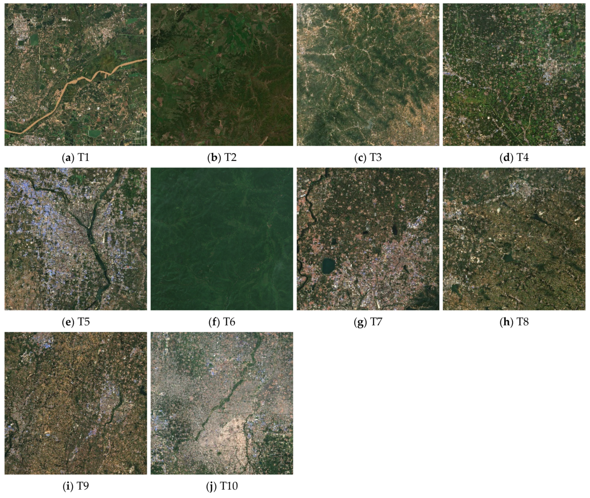
2.1. Image Data and Preprocessing

In the experiments, 10 images of different places from the Copernicus Open Access Hub [42] were collected. To fully evaluate the proposed strategy, the criteria for selecting images was that the landscape categories should vary greatly from each other. Each scene was cropped to 4096 × 4096 cells with three bands (red, green, and blue). The 10 images were acquired in 2020 and are designated T1 to T10, respectively. As can be seen in Figure 1, the landscape patterns of these images are diverse and include an urban area, villages, forests, mountains, croplands, prairies, wetlands, and vegetable greenhouses.

The region growing and watershed algorithms were employed to evaluate the proposed strategy, given that the algorithms have demonstrated acceptable segmentation performance in broad applications and have been used at the pretreatment stage in various image processing procedures [43,44,45,46,47]. The algorithms were constructed according to Adams and and Bischof [40] and Vincent and Soille [41]. Both of the algorithms are seed-based algorithms, as the programs start growing from the seed points every time. The parameters for the preprocessing of the input images are presented in

Table 1. Parameters used for the preprocessing of input images.

Algorithm	Bands	Median Radius	Spectral	Seed Points	Tile Size Range
Region growing	2	2 pixels	Grayscale	Local peaks	4
Watershed	2	2 pixels	Gradients	Gradient threshold	4

, and the preprocessing operations are described below.

The input image for both algorithms consisted of two bands, namely the spectral band and the seed points band. In terms of the spectral band, the three true color bands for each image were first converted to the single grayscale band by forming a weighted sum of the red, green, and blue band components, as detailed in Equation (1) according to the function rgb2gray in MATLAB [48]. Afterwards, all single band images were processed with a median filter to remove image noise with a radius of two pixels. The spectral band for the watershed method was the gradient image produced by the gradient function imported from the scikit-image package [49], while that for the region growing method was the original grayscale image. In terms of the seed points band, the seed points were generated by the threshold of the gradient image for the watershed method, while that for the region growing method was based on finding the local maximum and minimum peaks of the spectral band with a specific window size. The four groups of tiles ranged in size from 256 to 512, 1024, and 2048 pixels.

The reference (also called the ground truth) images were the segmented results generated in a sequential way. The reference images for different seed point densities and segmentation algorithms were diverse with respect to the 10 images:

Gray = 0.299 ∗ R + 0.587 ∗ G + 0.114 ∗ B

(1)

where R, G, and B represent the values from the red band, the green band, and the blue band, respectively; gray indicates the acquired grayscale value.

2.2. Methods

In this research, the distributed strategy was explored to implement the seed-based image segmentation algorithms over the Spark platform. The distributed strategy focused on modification of incomplete objects and a reasonable reduction of the inner communication volume during the shuffle stage. Details of the proposed strategy and the performance evaluation are given in the following sections.

2.2.1. Overview

An overview flowchart of the distributed strategy is presented in Figure 2. The flowchart consists of six main parts; that is, image pretreatment, tile segmentation, buffer size detection, auxiliary band synthesis, border area processing, and tile integration. The buffer size detection and auxiliary band synthesis are discussed in detail in Section 2.2.2 and Section 2.2.3, respectively. First, the Spark platform loads in the large image and decomposes the image into multiple tiles with a desired shape. The tiles are encapsulated into a Spark RDD (resilient distributed dataset) structure, which distributes the tiles to designated calculation nodes. Second, the seed-based segmentation algorithms are implemented over each tile independently. The buffer size detection obtains the maximum size of the border objects with respect to the total tiles, and then the border objects are masked to create the target mask areas via auxiliary band synthesis. Afterwards, the auxiliary band records intermediate data and the spectral bands are shuffled to transform the buffered tiles as needed over the distributed cluster. Third, all tiles are extended with auxiliary and spectral bands in their neighbors and the seed-based segmentation algorithms are implemented on the mask areas of the tiles in the border area processing stage. Finally, the tile integration step acquires the cropped tiles from each calculation node to generate the final results.

The tiles distributed over multiple calculation nodes acquire spectra, seed points, categories (indicating the index of objects), border lines, and directions (indicating the relative locations of objects within each tile, including the upper, the right, the lower, and the left) from the neighboring tiles to modify the incomplete objects. This procedure demands data transformation and creates the most communication volume among the designated calculation nodes. In general, the available communication bandwidth is not large enough compared to the transformed volume of the buffered tiles. The communication issue places limits on achieving high-performance parallel image processing. Decreasing unnecessary data transformation among the calculation nodes is an effective way to reduce the communication volume and enhance the performance over the Spark platform. Therefore, the primary objectives are to reduce the communication volume in a reasonable manner and to achieve execution efficiency with high accuracy. The two main solutions are described in the following sections.

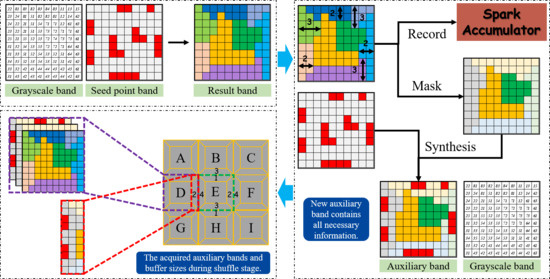
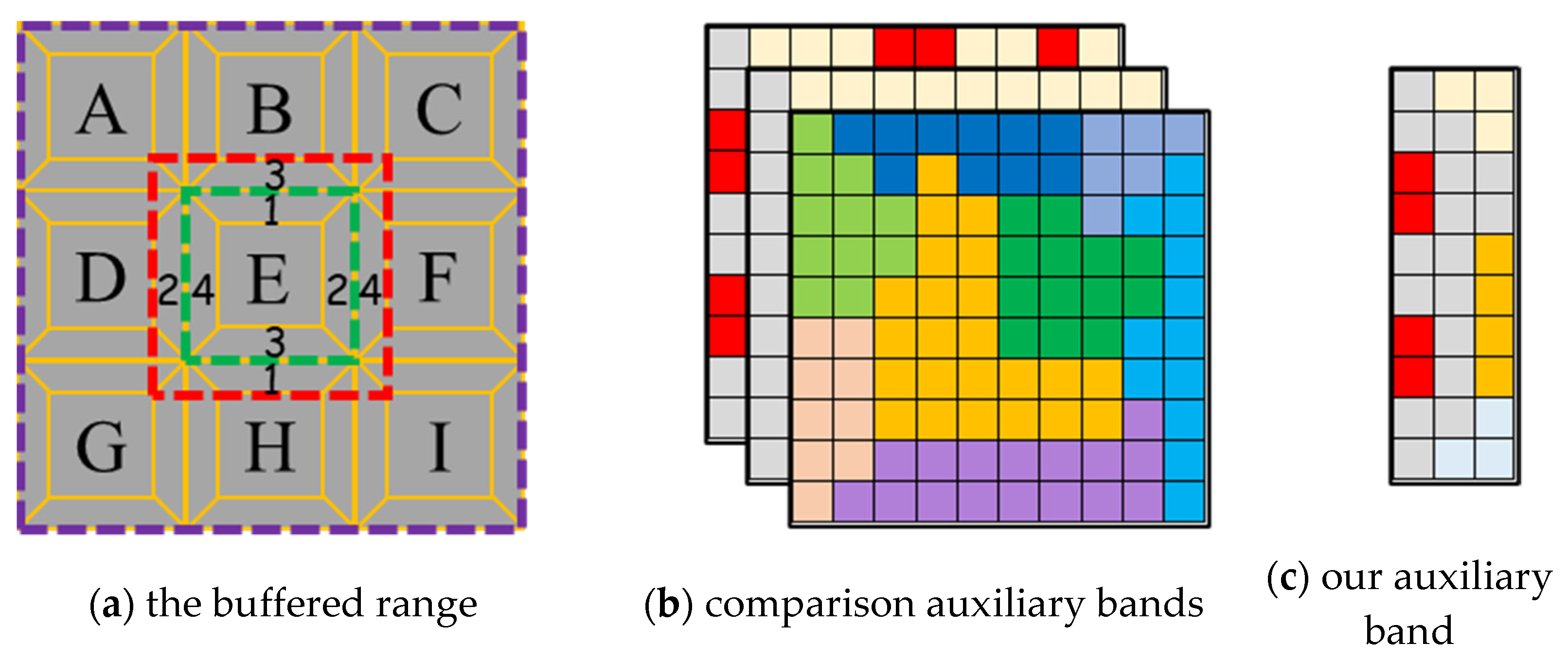
2.2.2. Automatic Buffer Size Detection

One of the solutions for decreasing the communication volume is to estimate the buffer size accurately, rather than simply assuming a large enough threshold, as was done by Derksen, Inglada [36]. Clearly, the communication volume generated by the tile shuffle operation may be determined partly by the buffer size. A larger threshold value for the buffer size may lead to a heavy communication volume among the calculation nodes.

The function of the buffer size detection workflow over the distributed cluster is to detect and record the maximum length or width of the border objects around the four aspects in each tile. Each tile acquires four buffer sizes and the maximum one is selected as the return value of the automatic buffer size detection operation. The maximum of the return values integrated from each tile is the desired maximum buffer size. This workflow deals with the issue using distinct logic compared with that used in a single machine. As the tiles are distributed in multiple calculation nodes, the maximum buffer size of each tile cannot be returned directly from each calculation node to the master node over the distributed cluster. Hence, accumulators in the Spark platform are imported to solve the problem. Accumulators are basically write-only structures and allow us to aggregate the desired values from the calculation nodes to the master node. In our program, the accumulator records the maximum buffer size in a parallel manner in each calculation node and integrates the acquired values to the master node by the numeric list.

However, the numeric list is not returned to the master node immediately, as the operating mechanism of the Spark platform by default is a lazy calculation [50,51]. In the Spark platform, two basic types of Spark RDD operations are used to deal with the various datasets, namely transformations and actions [52]. The transformations produce new RDDs from the existing ones, while the actions acquire non-RDD values from the given RDDs [53]. The program does not process datasets until the action operation is triggered. Hence, the accumulator does not acquire any buffer size values in the transformation stage until the action operation is called.

To obtain the maximum buffer size, the action operation needs to be called after the tile segmentation and before the border area processing stage. The program processes the tiles and obtains the maximum buffer size when it meets the action operation, such as the count operation. Furthermore, the persist operation is also called to save the results of the first action operation in the CPU to avoid unnecessary recalculation, as each action operation would implement the total program fragment from the beginning to the current position without the persist operation [54]. Therefore, the maximum buffer size could be used to acquire the buffered tiles in each calculation node before the border area processing stage. The automatic buffer size detection mechanism is implemented in the distributed cluster.

2.2.3. Auxiliary Band Synthesis

Another solution for reducing the communication volume greatly is to limit the number of auxiliary bands. This is because the communication volume generated by the tile shuffle operation could be also partly determined by the number of auxiliary bands. A large number of auxiliary bands for buffered tiles gives rise to larger communication volumes relative to that of fewer auxiliary bands with the same buffer size.

The auxiliary bands are created to record the intermediate data during the tile processing, as reported by Wang, Chen [18]. The intermediate data need to be saved and transformed because these data would guide the following procedures. As mentioned in Section 2.1, the input images consisting of two bands store the spectrum and seed points, respectively. Neither of these could be reduced during the tile shuffle stage because they would be used several times in the following procedures. Therefore, synthesizing the intermediate data into the seed points bands is one of the feasible solutions to reduce the communication volume.

In a previous study [18], three auxiliary bands were imported to record the border lines, categories, and directions, respectively. In our distributed strategy, the three types of data recorded separately in three auxiliary bands were all synthesized to a single auxiliary band in each tile in a reasonable manner. As can be seen in Figure 2, step ④, this presents the generation procedure of a new auxiliary band. The auxiliary band is produced by implementing the seed-based segmentation algorithms to process each tile independently over the distributed cluster. The band consists of the categories and their corresponding border lines. The seed point band records the seed points of the tiles. The categories and the surrounding border lines located in the inner tiles remain, while those located in the four border aspects comprise the border areas in each tile. Next, the border area objects are masked with four directions (the upper, the right, the lower, and the left) and marked with a specific signature in the intermediate band. At last, the seed points located in the border areas are masked and combined with the intermediate band to generate the new auxiliary band, which would replace the original seed points band.

The categories and directions marked in the new auxiliary band are the same as those proposed by Wang, Chen [18], while the border lines are used to distinguish various objects. As can be seen in Figure 3, with such a strategy, the categories, border lines, directions, and seed points are recorded by only one auxiliary band (Figure 3c) and not transformed among the calculation nodes via each corresponding individual band (Figure 3b) any more. The buffered tile E only acquires pixels from adjacent tiles with the intersection region of the red box and green box rather than that of the purple box and green box (Figure 3a). Furthermore, the new auxiliary band would be transformed with the input spectral band together in the shuffle stage. As a result, all of the above-mentioned information would be transformed via two bands without any increment of the auxiliary band for use in seed-based segmentation algorithms.

2.2.4. Performance Evaluation

The performance of the proposed strategy was evaluated to assess the accuracy and execution efficiency. In terms of the accuracy assessment, this was evaluated using the F-measure metric [55] as expressed in Equation (6). The F-measure consists of two basic components—the recall and precision metrics, as presented in Equations (4) and (5), and the object matching criteria [56,57], as defined in Equation (2). The F-measure was then acquired based on the following metrics given by Equations (2)–(6):

$$match=\arg max \left|S_i^s {\displaystyle \cap } S_k^r\right|$$

(2)

$$w_i=\frac{S_i}{{{\displaystyle \sum }}_{i=1}^n{S}_i}$$

(3)

$$Precision={\displaystyle \sum }_{i=1}^{n_s}{w}_i\frac{\left|S_i^s {\displaystyle \cap } S_{match}^r\right|}{\left|S_i^s\right|}$$

(4)

$$Recall={\displaystyle \sum }_{i=1}^{n_r}{w}_i\frac{\left|S_i^r {\displaystyle \cap } S_{match}^s\right|}{\left|S_i^r\right|}$$

(5)

$$F\text{-}measure=\frac{1}{\frac{\alpha }{Precision}+\left(1-\alpha \right) \frac{1}{Recall}}$$

(6)

where $S_i^s$ and $S_i^r$ are the sets of pixels in the $i$-th segment object and reference object, respectively; $n_s$ and $n_r$ are the object numbers of segment objects and reference objects, respectively; $w_i$ is the weight factor of the $i$-th object; $S_{match}^r$ and $S_{match}^s$ are the sets of pixels in the matching reference and segment object, respectively; α is a constant and =0.5; and the values of the F-measure range from 0 to 1.

In terms of execution efficiency, the variability in the execution time of the proposed strategy against the same scene images for different auxiliary bands and buffer sizes are evaluated. The settings for the number of calculation nodes in all experiments are based on the experimental results carried out in the beginning of Section 3.2.

3. Results

The accuracy and execution efficiency are assessed in the following sections.

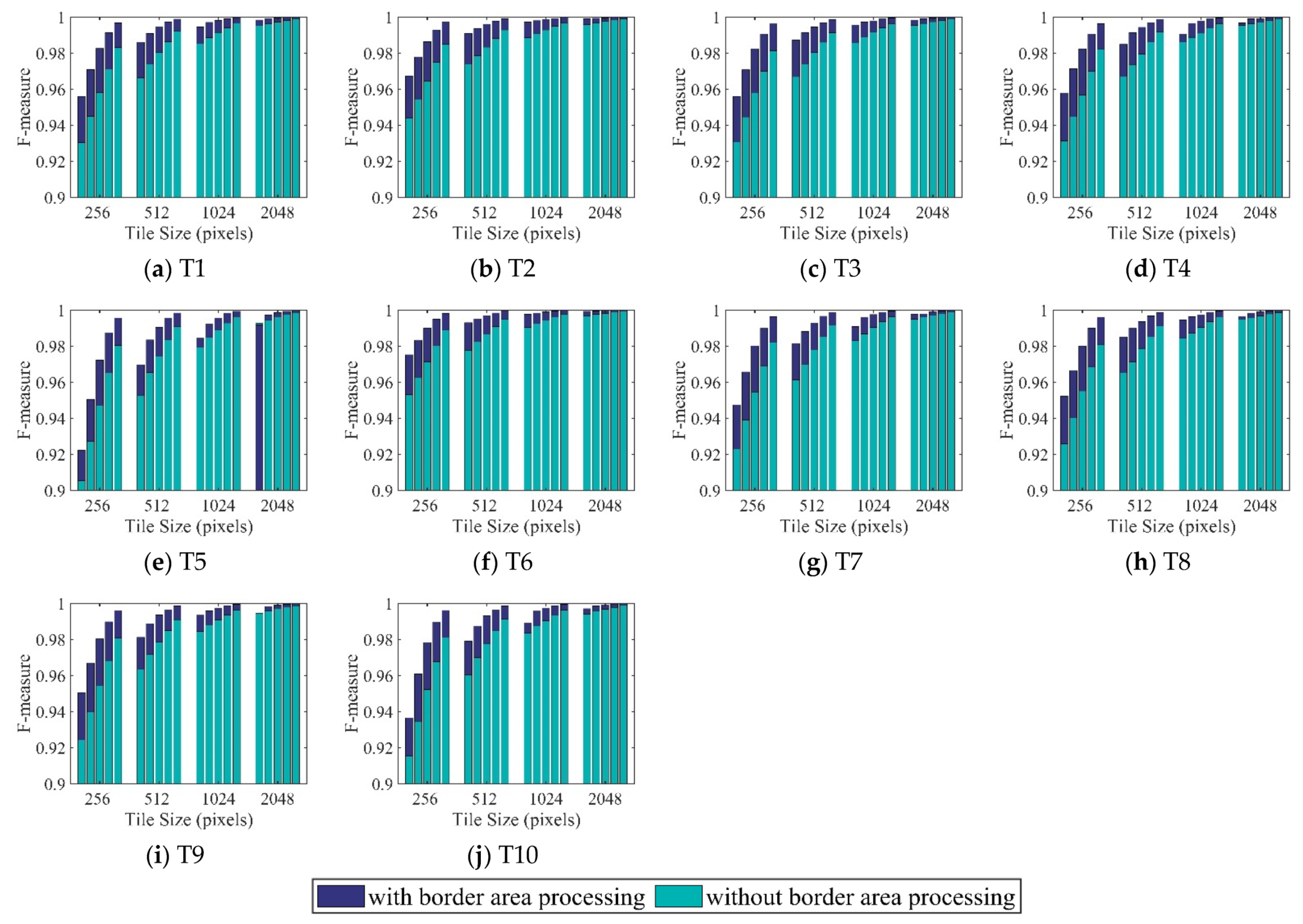
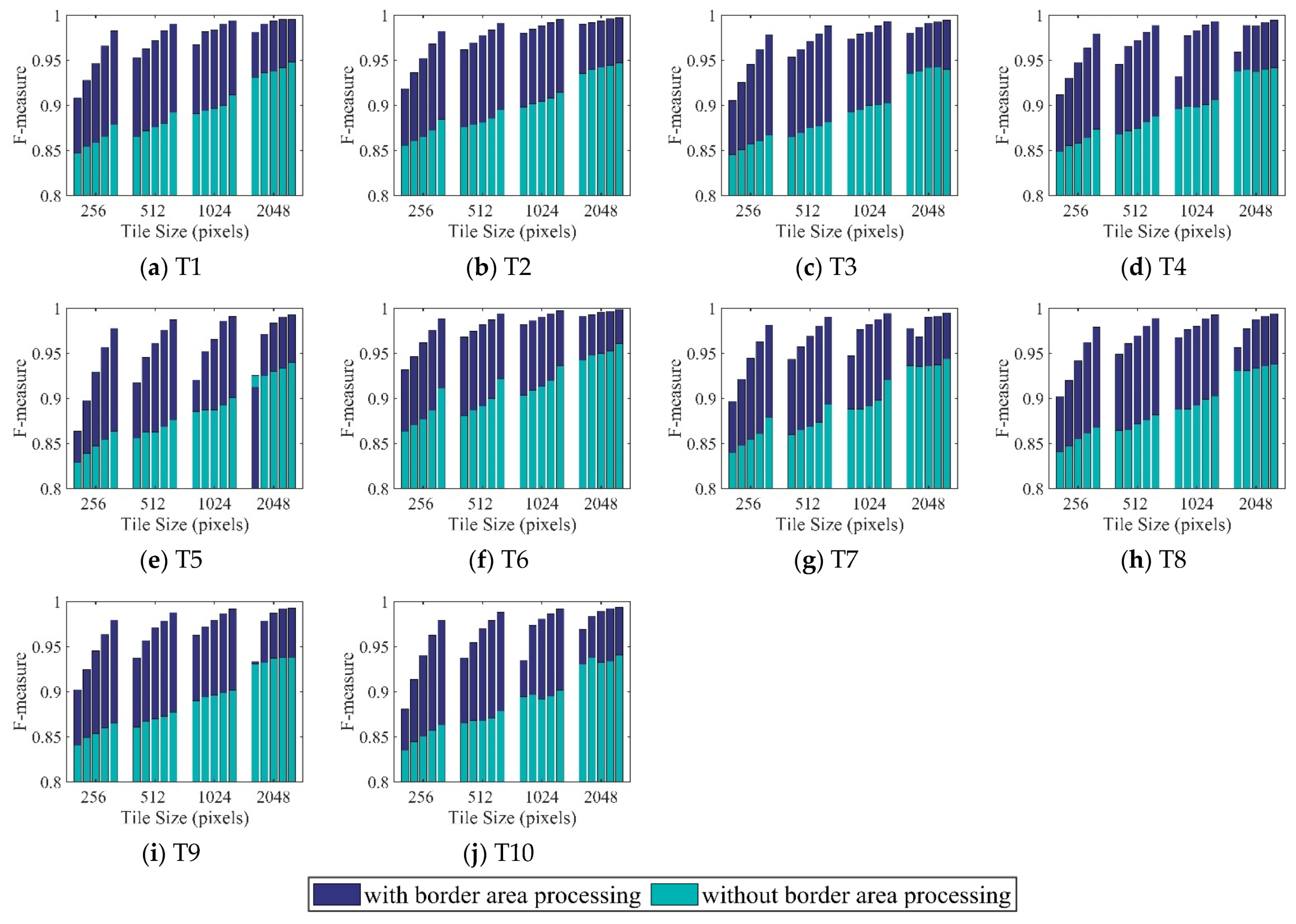
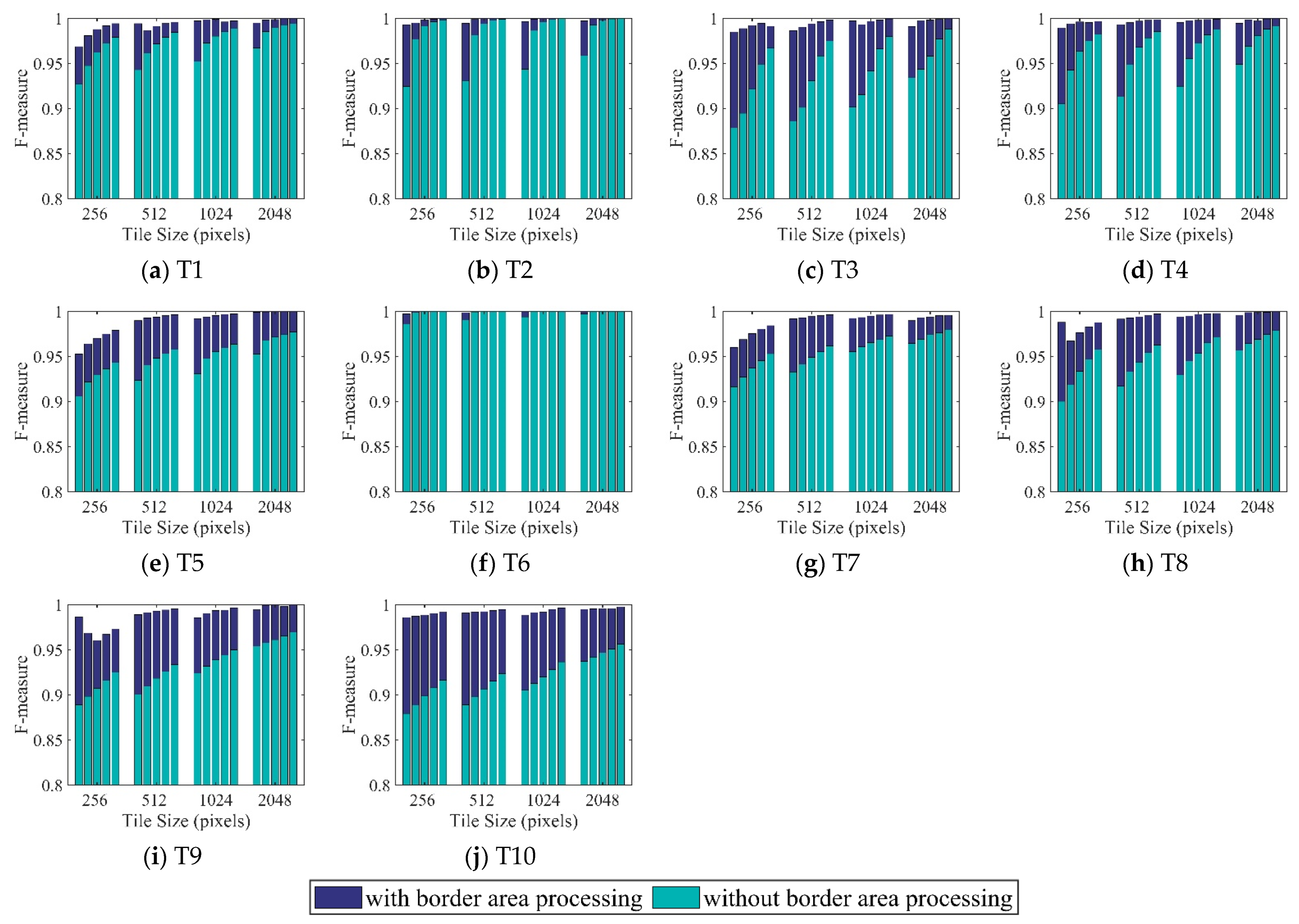
3.1. Results for Accuracy Assessment

The experimental results produced by a single machine are treated as the reference image, and these results are used to evaluate the results generated by the distributed cluster. In this study, two groups of comparisons are set for both the region growing and watershed algorithms. In the first group, the entire objects generated by the distributed cluster with and without border area processing are extracted and compared with the reference objects. Clearly, however, the accuracies are all too high to distinguish the variation. In the second group, the border areas in each tile are extracted and regarded as the border mask. The objects generated by the distributed cluster with and without border area processing are extracted according to the border mask. These border objects are also adopted to make accuracy comparisons with the corresponding objects in the reference images.

To evaluate the accuracy of the distributed strategy for the region growing and watershed algorithms, comparisons of the density levels of the five groups of seed points for each algorithm were undertaken. As illustrated in

Table 2. The seed point density levels for the two algorithms.

Algorithm	Level 1	Level 2	Level 3	Level 4	Level 5
Region growing	33 × 33	27 × 27	21 × 21	15 × 15	9 × 9
Watershed	Gradient < 2	Gradient < 3	Gradient < 4	Gradient < 5	Gradient < 6

, the seed point density increases gradually from level 1 to level 5. Accuracy assessments of both segmentation algorithms with and without border area processing are illustrated in Figure 4, Figure 5, Figure 6 and Figure 7. The four groups of figures present the accuracy assessments of (1) the entire image using the region growing method, (2) the border image using the region growing method, (3) the entire image using the watershed method, and (4) the border image using the watershed method. Accuracy assessments of the entire image and the border image correspond to the first and second groups of comparisons, respectively.

The accuracy assessments in terms of the entire image using the region growing method with and without border area processing are illustrated in Figure 4. In all images, the accuracy rises gradually along with the seed point density from level 1 to level 5 over each tile size group. The largest and least accurate increment from level 1 to level 5 of seed point density occurred in tile size groups 256 and 2048, respectively. In each seed point density level, the accuracy rises across the tile size groups from 256 to 512, 1024, and 2048 in each subfigure. The accuracy increment from tile sizes 256 to 512 was the largest, while that from tile sizes 1024 to 2048 was the smallest. The accuracies with border area processing were higher than those without border area processing in almost subfigures, except the first bin in tile size group 2048 in Figure 4e. The accuracy differences in almost all cases decreased gradually, along with not only the tile sizes increasing from 256 to 512, 1024, and 2048, but also the seed point density varying from level 1 to level 5. The differences in accuracy ranged from 0.02% to 2.7%, except for one outlier with a value of −0.1%. Meanwhile, the mean accuracies of the first bin in tile size 256 with and without border area processing were 95.2% and 92.8%, respectively.

The accuracy assessments in terms of border images using the region growing method with and without border area processing are shown in Figure 5. In all images, the accuracy rises gradually along with the seed point density from level 1 to level 5 in most tile size groups. In general, the largest and smallest accuracy increments of the seed point density from level 1 to level 5 occurred in tile size groups 256 and 2048, while those without border area processing exhibited insignificant variations in accuracy. At each seed point density level, the accuracy values with and without border area processing rose monotonously across the tile size groups from 256 to 512, 1024, and 2048 for most subfigures. For the monotonously increasing groups with border area processing, the accuracy increment from tile sizes 256 to 512 was the largest, while that from tile sizes 1024 to 2048 was the smallest. However, the situation varied for most groups without border area processing. The accuracies with border area processing were larger than for those without border area processing in almost subfigures except the first bin in tile size group 2048 in Figure 5e. The differences in accuracy did not exhibit any clear trends for increases in tile sizes from 256 to 512, 1024, and 2048, neither for variations in the seed point density from level 1 to level 5. The differences in accuracy ranged from 0.2% to 11.6%, except for one outlier with a value of −1.3%. Meanwhile, the mean accuracies of the first bin in tile size 256 with and without border area processing were 90.2% and 84.4%, respectively.

The accuracy assessment for the entire image using the watershed algorithm with and without border area processing is illustrated in Figure 6. In all images, the accuracy level with and without border area processing increased along with the seed point density from level 1 to level 5 in most cases and in all cases separately in each tile size group. In most cases, the largest and smallest accuracy increments of the seed point density from level 1 to level 5 occurred in tile size groups 256 and 2048. At each seed point density level, the accuracy increased across the tile size groups from 256 to 512, 1024, and 2048 in almost all subfigures. In general, the accuracy increment from tile sizes 256 to 512 was the largest, while that from tile sizes 1024 to 2048 was the smallest. Accuracies with border area processing were higher than those without border area processing in all subfigures. In most cases, the differences in accuracy decreased gradually not only with increase of tile sizes from 256 to 512, 1024, and 2048, but also for the varying seed point density from level 1 to level 5. The differences in accuracy ranged from 0.001% to 0.8%. Meanwhile, the mean accuracies of the first bin in tile size 256 with and without border area processing were 99.8% and 99.1%, respectively.

The accuracy assessments in terms of the border image using the watershed method with and without border area processing are shown in Figure 7. In all images, the accuracies with border area processing increased slightly, while those without border area processing increased significantly along with the seed point density from level 1 to level 5 for most tile size groups. For each seed point density level, the accuracy increased across the tile size groups from 256 to 512, 1024, and 2048 for almost all subfigures. In most cases, the accuracy increments exhibited no obvious trends with respect to the growth of the tile size or the increase in the seed point density. The accuracies with border area processing were higher than those without border area processing in all subfigures. In almost all cases, the least accurate differences occurred in tile size group 2048. The differences in accuracy ranged from 0.001% to 10.7%. Meanwhile, the mean accuracies of the first bin in tile size 256 with and without border area processing were 98.1% and 91.1%, respectively.

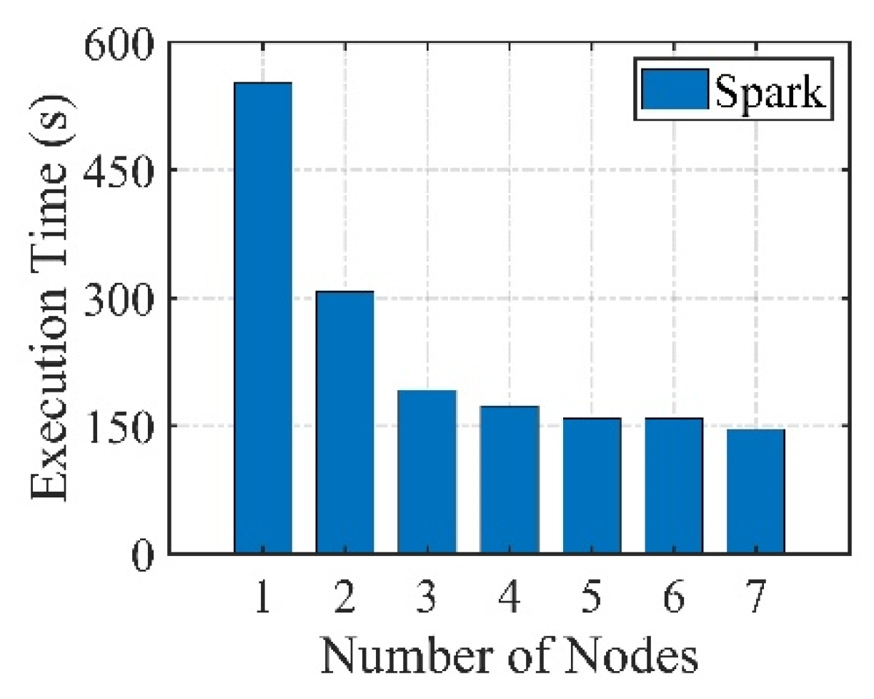
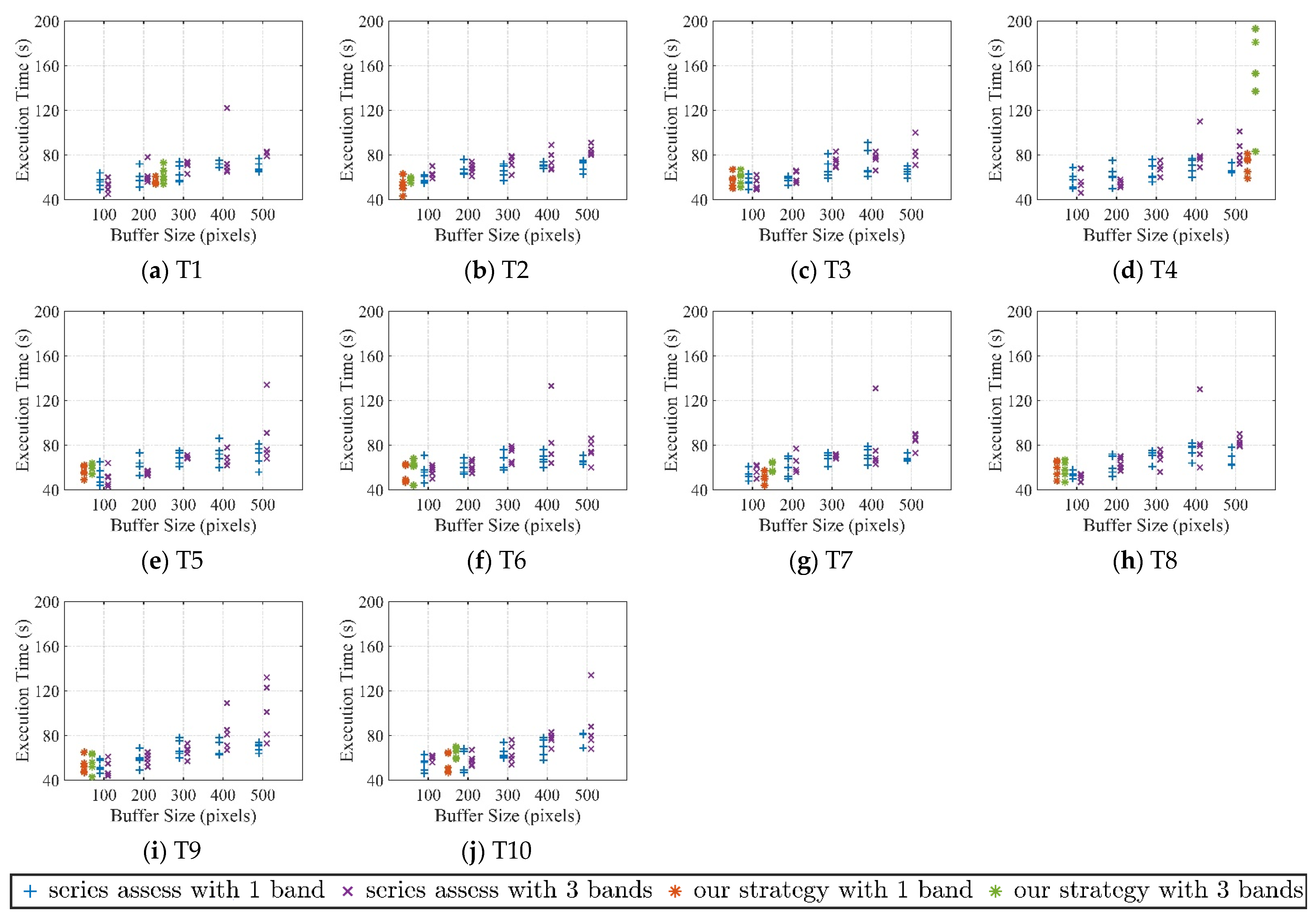
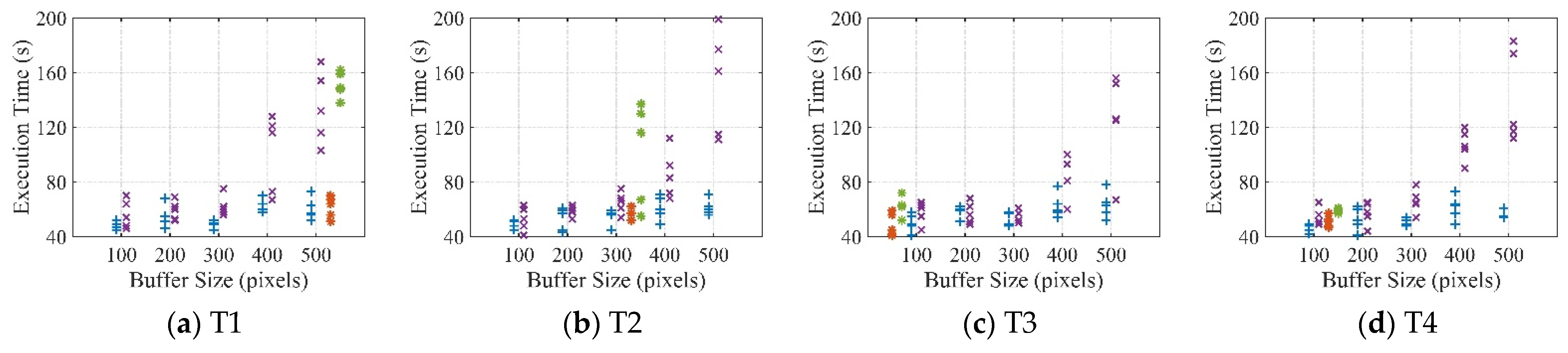
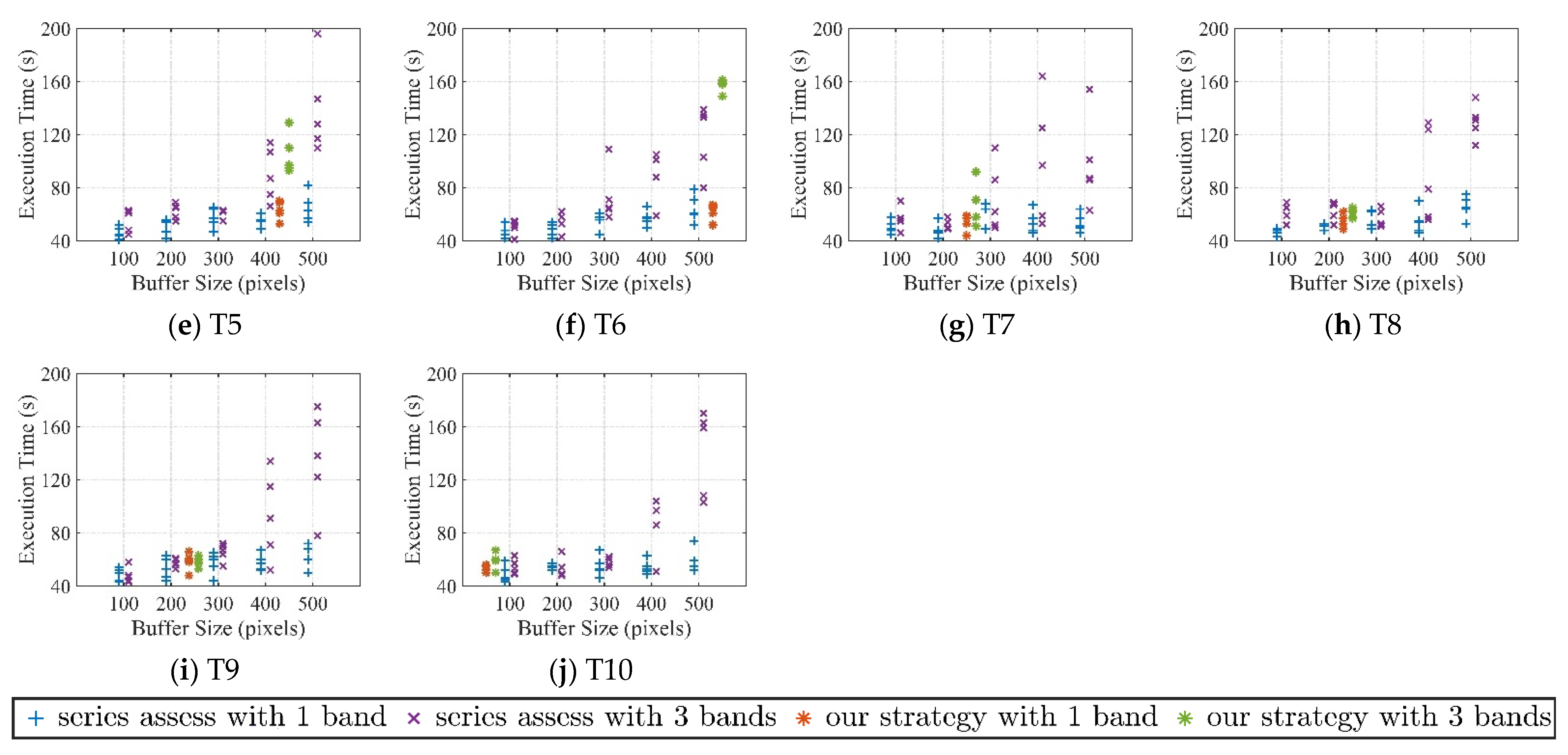
3.2. Results for Execution Efficiency

In this study, the efficiencies for both the region growing and the watershed methods are indicated by the execution time. The best number of calculation nodes is first evaluated over one image with 4096 × 4096 cells. Given that there are seven physical calculation nodes in the distributed cluster in total, the numbers of calculation nodes range from 1 to 7 with a tile size of 512 × 512, an executor number of 1, and an executor memory of 2G. As can be seen in Figure 8, in general the execution time decreases with increasing numbers of calculation nodes.

As time elapses, a rapid decrease occurs for the first three bins, a gradual decrease for the middle two bins, and an erratic response in the last two bins. At the beginning, an increment in the calculation nodes could bring effective CPU to reduce the insufficient calculation power. In the middle stage, the communication volume also increases as the number of calculation nodes increases. However, strengthening of the calculation nodes outweighs the cost of the communication volume, and the execution time is still decreasing gradually. In the last stage, the cost of the communication volume continues to increase and exceeds the contribution of the calculation nodes, such that the execution time becomes unstable and the decrease in magnitude becomes weak. An increase of the calculation nodes at this stage would not greatly decrease the execution time. Hence, the number of calculation nodes was set as 4 in the following experiments.

To illustrate the advantages of having an improved execution efficiency for the distributed strategy, comparisons of the execution time were made by selecting various auxiliary bands and buffer sizes. In addition, the execution time was compared with another parallel strategy proposed by Wang, Chen [18] rather than that of algorithm implemented in a sequential way. For the images presented in Figure 1, the number of auxiliary bands for comparison purposes were set as 1 and 3, and the buffer size was based on automatic detection and manual settings, respectively. As a result, each of the subfigures includes four types of values, comprising (1) the manual buffer size setting with one auxiliary band, (2) the manual buffer size setting with three auxiliary bands, (3) the automatic buffer size with one auxiliary band, and (4) the automatic buffer size with three auxiliary bands. The manual settings comprised five groups of buffer size ranging from 100 to 500 in increments of 100, while the automatic buffer size plot values were based on the number of pixels practically available. Ten images with various landscape patterns were available; therefore, the automatic detection buffer size of each image for both segmentation algorithms was variable, with the sizes listed in

Table 3. The buffer sizes for automatic detection of the two segmentation algorithms for T1 to T10.

Algorithm	T1	T2	T3	T4	T5	T6	T7	T8	T9	T10
Region growing	204	46	97	512	96	53	123	89	86	182
Watershed	512	341	73	108	440	512	298	228	248	85

. Given that the operations of the distributed cluster were unstable, each buffer size for T1 to T10 was tested five times, which gave a total of 1200 for all cases. The settings of the Spark submit routine were as follows. Four executors were adopted in the experiment with four executor cores for each and 2G executor memories with the tile size 512; the driver memory and the size for the maximum result were both set as 15G.

The acquired elapsed time for the region growing and watershed methods are listed in Figure 9 and Figure 10, respectively. In general, the overall execution time for all subfigures (Figure 9 and Figure 10) increases as the buffer size grows from 100 to 500 for both cases with one and three auxiliary bands. The time increment for the watershed method is clearer compared to that for the region growing method, while the total execution time of the region growing method is less than that for the watershed method. The time gaps between the cases with one and three auxiliary bands also vary among the 10 images. The execution times of almost all cases with three auxiliary bands are larger than those with one auxiliary band, a finding which is particularly evident in the buffer size groups of 400 and 500. For automatic buffer size detection, almost all cases with three auxiliary bands take longer than those with one auxiliary band when handling the same image. There are usually outliers present in the subfigures, with those conditions being imported as a result of the instability in the distributed cluster. Decreasing trends among two adjacent buffer size groups exist, although the trend overall is a gradual increase. On the one hand, the execution time produced by the proposed strategy is less than that for three auxiliary bands in most cases. On the other hand, in general, the execution time of the automatic detection buffer size is less than that of the nearest manually applied buffer size selection.

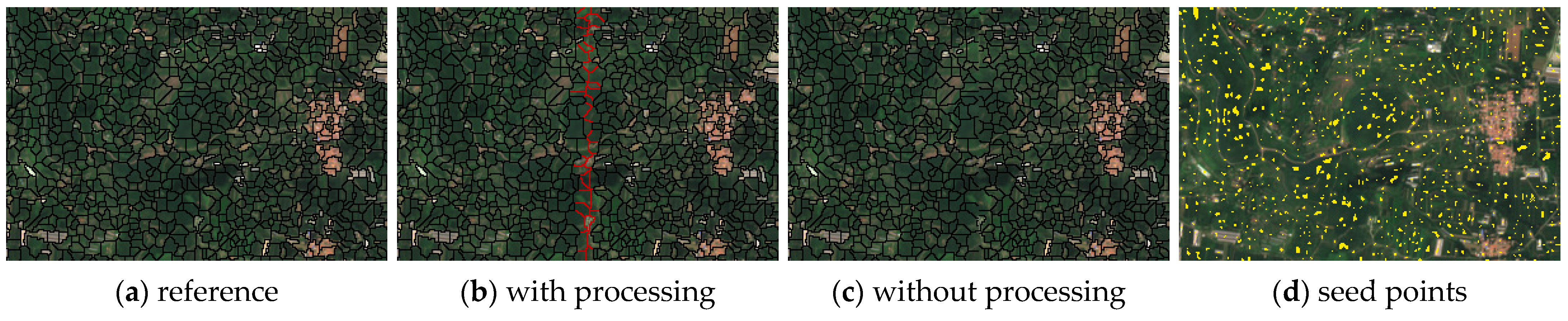
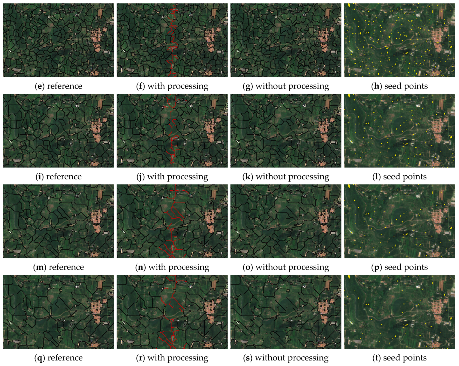
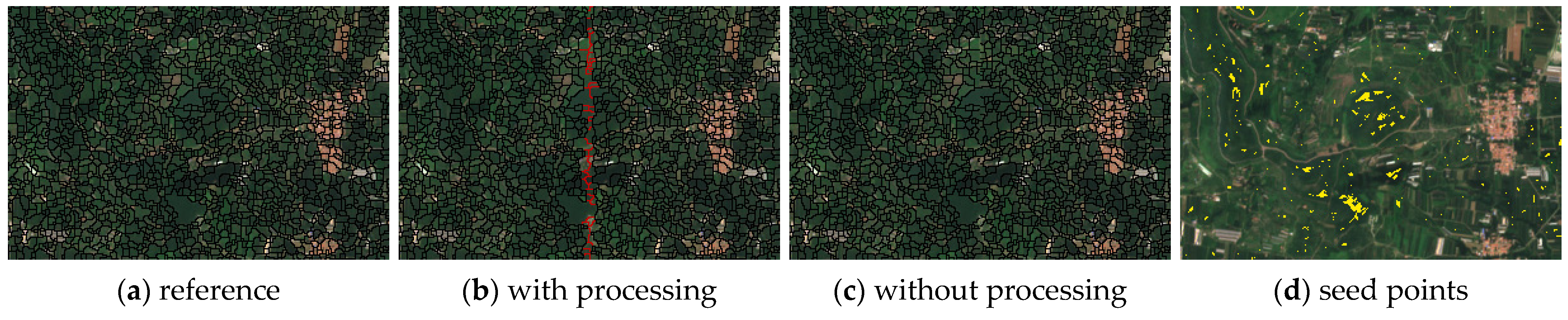
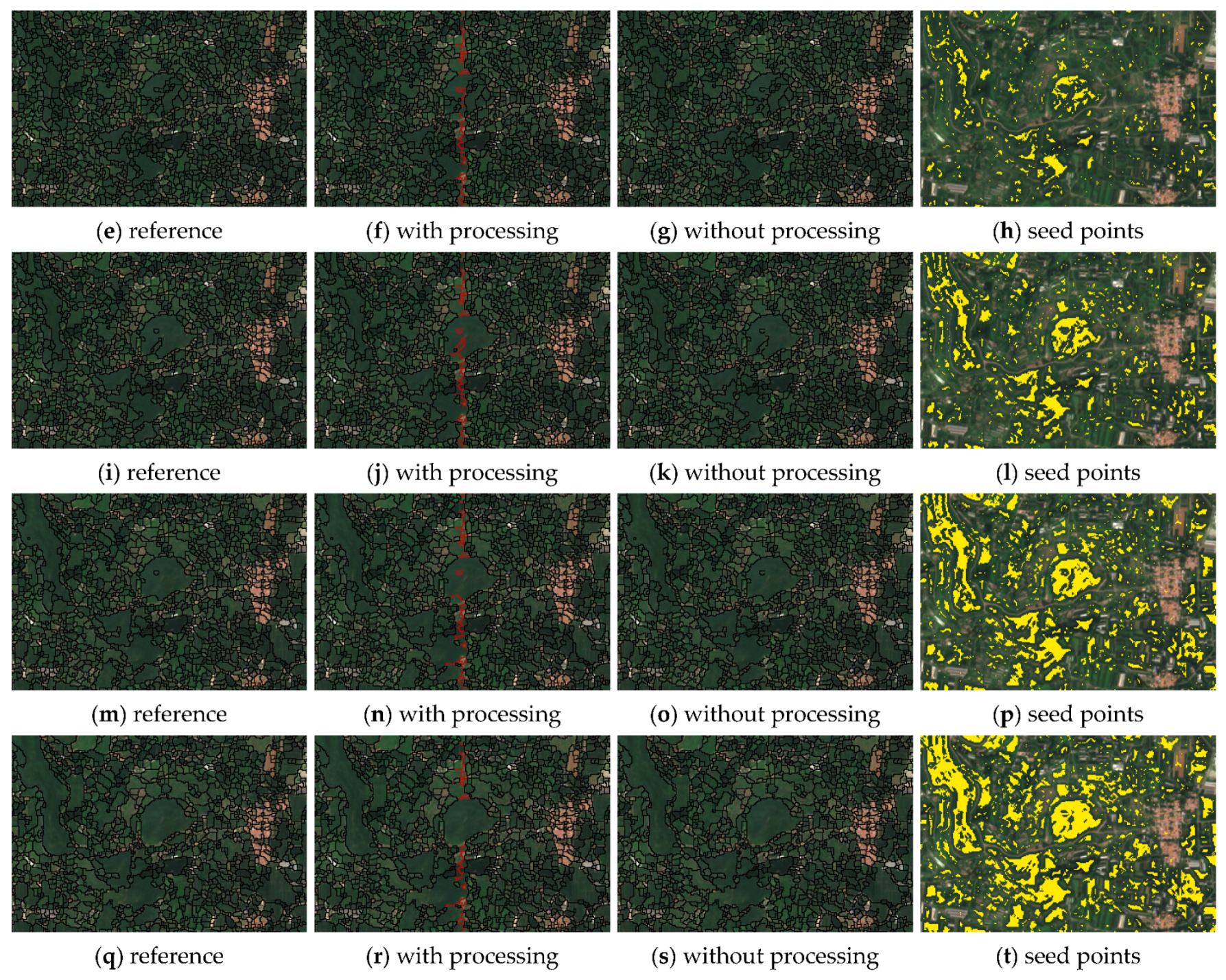
3.3. Results of Visual Comparison

To demonstrate the patterns of segmentation results with five different seed point density levels, the subset image results generated by the region growing and watershed methods for T10 in Figure 11 and Figure 12 are illustrated for comparison purposes. The performances of the proposed strategy can be clearly seen. Objects in the images are outlined with black border lines, the modified border area objects are marked with red border lines, and the seed points are marked in yellow. According to Figure 11 and Figure 12, the inner objects generated by the region growing and watershed methods are identical to those in the corresponding reference image. The border objects are quite similar to those in the corresponding reference image. For the segmentation results generated by the region growing method (Figure 11), the object sizes become increasingly larger as the seed point density decreases from level 5 to level 1. For the segmentation results produced by the watershed method (Figure 12), the object sizes become larger as the seed point density increases from level 1 to level 5. The object sizes for the region growing results for each seed point density level are relatively uniform, while there are significant differences for the watershed results and only part of the objects become larger as the seed point density increases. Meanwhile, the seed point characteristics for each segmentation algorithm are the same as those for the object sizes discussed previously. The artifacts in the border areas for both segmentation results are generally eliminated. Thus, the results reveal that the seed-based segmentation algorithms are suitable for implementation over the distributed cluster.

4. Discussion

Both the accuracy levels with and without border area processing are higher than those achieved in previous work [18]. This is due mainly to the characteristics of the two seed-based image segmentation algorithms. The processing sequences for the seed-based algorithms first grow the candidate pixels surrounding the seed points, then handle the remaining candidate pixels. Furthermore, the seed-based objects may grow from the same seed points into the same shape with approximately identical pixels, regardless of whether the seed-based objects are located in the inner or border regions of the tile. Therefore, the seed-based algorithms ensure that accuracy is higher for all images.

The density of the seed points also influences the accuracy greatly. In general, the larger the seed point density, the better the performance. A larger seed point density means that the seed points occupy a higher ratio of the entire image. In other words, a larger seed point density leads to more seed-based objects and fewer non-seed-based objects, which may be regarded as being produced by a random growing sequence. The ideal solution is that each object is grown from unique seed points, such that the entire image is constructed from these objects. However, different types of seed points play different roles in the processing stage. The seed points of the region growing method clearly make the size and distribution uniform. Hence, the accuracy of the region growing method would increase linearly with an increase in the seed point density in almost all circumstances. The seed points of the watershed method are influenced mainly by the characteristics of the image pattern. The size and distribution of seed points is non-uniform, as there are various images. In addition, the increment of seed points between every two levels is approximately scalable for the region growing method, while that for the watershed method is nearly random in each image. Accuracies for the watershed method could not increase linearly with increases in the seed point density from level 1 to level 5, as the higher density regions would go on increasing while the lower density regions would still lack seed points in many cases. The accuracy levels among the same seed point density levels for the region growing method show few variations, while accuracy levels vary greatly for the watershed method. For the same seed point density level, the greater the seed point density, the higher the accuracy.

As seen in the evaluation of the execution efficiency, the decreasing patterns of the adjacent buffer size groups are caused mainly by the image volume and the hardware conditions of the distributed cluster. On the one hand, when the image volume is small, the memory size and the capability of the CPU are sufficiently powerful to handle the images relative to the memory occupied by the processing procedure. Hence, the variation of execution time between buffer size groups 200 and 300 is mainly governed by the cluster states, which influence the execution time more than the original image volume. On the other hand, the buffer size gaps utilized in the experiment are relatively small and the increment volume is not large enough to influence the execution time. For example, although decreasing trends occurred in adjacent groups in Figure 9c–e, this condition is not manifested in buffer size groups 100 and 500, which could be regarded as the evidence. Hence, it is necessary to apply automatic buffer size detection in the strategy, as can be seen in Figure 9 and Figure 10. The largest increment in time for the buffer size groups from 100 to 500 could be approximately 100 s for an image of 4096 × 4096 cells (the proposed strategy runs twice as fast as the one without communication volume reduction), while the increase in time could be greater as the tile size gets larger.

In this study, we did not record or analyze the computational complexity. The computational complexity is affected by various factors in our six processing steps, mainly influenced by the adopted segmentation algorithms. Different segmentation algorithms would generate different computational complexity levels for the distributed strategy. The differences among various segmentation algorithms depend on the characteristics. Hence, the computational complexity of the distributed strategy is ignored. In terms of the reliability, this research takes two seed-based segmentation algorithms; ten testing images, including various landscapes; and 5 testing times for each variable (collecting a total of 1200 data points for all cases) to verify the performance of the distributed strategy and guarantee the reliability of the experiment results. The experimental designs could reduce the influences of unstable factors with respect to the execution time and could provide dependable data. Furthermore, the variation trends for the execution time are similar to each other in all study areas. In summary, our experimental results could be considered to be reliable.

According to the verification results of the proposed strategy, the memory calculations adopted in this experiment are the smallest so that the three auxiliary bands can handle the test images successfully, however when only one auxiliary band is adopted it is not the smallest. In some cases, the distributed strategy could be implemented with relatively smaller calculation memory, while the programs with three auxiliary bands would not be able to satisfy the execution conditions. Therefore, the distributed strategy affords not only a higher execution efficiency but also lower hardware requirements. This means that the proposed strategy has a powerful capability to handle very large remote sensing images. However, if we are talking about a complex method that only makes minor improvements to a very small number of objects, its computational complexity might not be so clearly justifiable.

5. Conclusions

The distributed image processing algorithms may handle very large remote sensing images efficiently. Employing the sequential algorithms using the Spark platform is an effective way to handle large images over the distributed clusters. However, the sequential algorithms employed directly by the Spark platform over the distributed cluster may lead to significant problems in terms of accuracy and efficiency. Specifically, the incomplete objects generated in the tile edges result in a decrease in accuracy and the large communication volume in the inner Spark platform reduces the execution efficiency.

To overcome these issues, the distributed strategy of seed-based segmentation algorithms, which focus on modifying the incomplete objects and optimizing the communication volume in the inner Spark platform, is proposed. In the distributed strategy, the additional communication volumes are optimized by addressing two aspects. On the one hand, the buffer size is detected automatically to limit the maximum buffer size for each tile. On the other hand, the auxiliary band numbers are synthesized into only one. Meanwhile, the incomplete objects are modified by implementing algorithms over the mask areas of the buffered tiles, including the spectral and auxiliary bands. Region growing and watershed algorithms are introduced to evaluate the performance in terms of the accuracy and execution efficiency. In the accuracy assessment, the results with border area processing exhibited better accuracy than those without border area processing. With respect to execution efficiency, tasks with significantly larger auxiliary bands and buffer sizes in general require more execution time than smaller ones. Therefore, the proposed strategy for using seed-based algorithms is to increase the accuracy and increase the execution efficiency effectively over the Spark platform. Moreover, the seed-based segmentation algorithms are suitable for implementation in the distributed strategy over the Spark platform.

In future work, the communication volume in the inner Spark platform should be quantified accurately by recording the execution time of the shuffle stage rather than the entire processing stage, given that the total execution time could be affected by many other compounding factors. The computational complexity of the proposed strategy will be recorded and analyzed in future studies. In addition, the buffer size is the same for the various tiles in this study, however each of the tiles needs a specific buffer size to further resolve the communication problems. The proposed strategy should be implemented with newer segmentation algorithms.

References

1. Li, F.P.; Feng, R.; Han, W.; Wang, L. High-Resolution Remote Sensing Image Scene Classification via Key Filter Bank Based on Convolutional Neural Network. IEEE Trans. Geosci. Remote Sens. 2020, 58, 8077–8092. [Google Scholar] [CrossRef]
2. Toth, C.; Jozkow, G. Remote Sensing Platforms and Sensors: A Survey. ISPRS J. Photogramm. Remote Sens. 2016, 115, 22–36. [Google Scholar] [CrossRef]
3. Zhou, D.C.; Xiao, J.; Bonafoni, S.; Berger, C.; Deilami, K.; Zhou, Y.; Frolking, S.; Yao, R.; Qiao, Z.; Sobrino, J.A. Satellite Remote Sensing of Surface Urban Heat Islands: Progress, Challenges, and Perspectives. Remote Sens. 2019, 11, 48. [Google Scholar] [CrossRef] [Green Version]
4. Happ, P.N.; da Costa, G.A.O.P.; Bentes, C.; Feitosa, R.Q.; da Silva Ferreira, R.; Farias, R. A Cloud Computing Strategy for Region-Growing Segmentation. IEEE J. Sel. Top. Appl. Earth Obs. Remote Sens. 2016, 9, 5294–5303. [Google Scholar] [CrossRef]
5. Chen, F.; Zhang, M.M.; Tian, B.S.; Li, Z. Extraction of Glacial Lake Outlines in Tibet Plateau Using Landsat 8 Imagery and Google Earth Engine. IEEE J. Sel. Top. Appl. Earth Obs. Remote Sens. 2017, 10, 4002–4009. [Google Scholar] [CrossRef]
6. Michel, J.; Youssefi, D.; Grizonnet, M. Stable Mean-Shift Algorithm and Its Application to the Segmentation of Arbitrarily Large Remote Sensing Images. IEEE Trans. Geosci. Remote Sens. 2015, 53, 952–964. [Google Scholar] [CrossRef]
7. Yan, L.; Roy, D.P. Improving Landsat Multispectral Scanner (MSS) Geolocation by Least-Squares-Adjustment Based Time-Series Co-Registration. Remote Sens. Environ. 2021, 252, 112181. [Google Scholar] [CrossRef]
8. Chen, F.; Zhang, M.M.; Guo, H.D.; Allen, S.; Kargel, J.S.; Haritashya, U.K.; Watson, C.S. Annual 30 m dataset for glacial lakes in High Mountain Asia from 2008 to 2017. Earth Syst. Sci. Data 2021, 13, 741–766. [Google Scholar] [CrossRef]
9. Yu, B.; Chen, F.; Xu, C. Landslide detection based on contour-based deep learning framework in case of national scale of Nepal in 2015. Comput. Geosci. 2020, 135, 104388. [Google Scholar] [CrossRef]
10. Chen, F.; Yu, B.; Li, B. A practical trial of landslide detection from single-temporal Landsat8 images using contour-based proposals and random forest: A case study of national Nepal. Landslides 2018, 15, 453–464. [Google Scholar] [CrossRef]
11. Apache Hadoop. Available online: http://hadoop.apache.org/ (accessed on 20 April 2021).
12. Apache Spark. Available online: http://spark.apache.org/ (accessed on 20 April 2021).
13. Guo, H. Big data drives the development of Earth science. Big Earth Data 2017, 1, 1–3. [Google Scholar] [CrossRef] [Green Version]
14. Mou, L.C.; Lu, X.Q.; Li, X.L.; Zhu, X.X. Nonlocal Graph Convolutional Networks for Hyperspectral Image Classification. IEEE Trans. Geosci. Remote Sens. 2020, 58, 8246–8257. [Google Scholar] [CrossRef]
15. Hong, D.F.; Yokoya, N.; Chanussot, J.; Zhu, X.X. An Augmented Linear Mixing Model to Address Spectral Variability for Hyperspectral Unmixing. IEEE Trans. Image Process. 2019, 28, 1923–1938. [Google Scholar] [CrossRef] [Green Version]
16. Zaharia, M.; Xin, R.S.; Wendell, P.; Das, T.; Armbrust, M.; Dave, A.; Meng, X.; Rosen, J.; Venkataraman, S.; Franklin, M.J.; et al. Apache Spark: A Unified Engine for Big Data Processing. Commun. ACM 2016, 59, 56–65. [Google Scholar] [CrossRef]
17. Kertesz, G.; Szenasi, S.; Vamossy, Z. Performance Measurement of a General Multi-Scale Template Matching Method. In Proceedings of the 2015-IEEE 19th International Conference on Intelligent Engineering Systems, Bratislava, Slovakia, 3–5 September 2015; pp. 153–157. [Google Scholar]
18. Wang, N.; Chen, F.; Yu, B.; Qin, Y. Segmentation of large-scale remotely sensed images on a Spark platform: A strategy for handling massive image tiles with the MapReduce model. ISPRS J. Photogramm. Remote Sens. 2020, 162, 137–147. [Google Scholar] [CrossRef]
19. Blaschke, T.; Hay, G.J.; Kelly, M.; Lang, S.; Hofmann, P.; Addink, E.; Feitosa, R.Q.; Van der Meer, F.; Van der Werff, H.; Van Coillie, F.; et al. Geographic Object-Based Image Analysis—Towards a new paradigm. ISPRS J. Photogramm. Remote Sens. 2014, 87, 180–191. [Google Scholar] [CrossRef] [PubMed] [Green Version]
20. Blaschke, T. Object based image analysis for remote sensing. ISPRS J. Photogramm. Remote Sens. 2010, 65, 2–16. [Google Scholar] [CrossRef] [Green Version]
21. Hussain, M.; Chen, D.; Cheng, A.; Wei, H.; Stanley, D. Change detection from remotely sensed images: From pixel-based to object-based approaches. ISPRS J. Photogramm. Remote Sens. 2013, 80, 91–106. [Google Scholar] [CrossRef]
22. Ventura, D.; Bonifazi, A.; Gravina, M.F.; Belluscio, A.; Ardizzone, G. Mapping and Classification of Ecologically Sensitive Marine Habitats Using Unmanned Aerial Vehicle (UAV) Imagery and Object-Based Image Analysis (OBIA). Remote Sens. 2018, 10, 1331. [Google Scholar] [CrossRef] [Green Version]
23. Pena, J.M.; Torres-Sánchez, J.; de Castro, A.I.; Kelly, M.; López-Granados, F. Weed Mapping in Early-Season Maize Fields Using Object-Based Analysis of Unmanned Aerial Vehicle (UAV) Images. PLoS ONE 2013, 8, e77151. [Google Scholar] [CrossRef] [Green Version]
24. Ma, L.; Li, M.; Ma, X.; Cheng, L.; Du, P.; Liu, Y. A review of supervised object-based land-cover image classification. ISPRS J. Photogramm. Remote Sens. 2017, 130, 277–293. [Google Scholar] [CrossRef]
25. Hossain, M.D.; Chen, D. Segmentation for Object-Based Image Analysis (OBIA): A review of algorithms and challenges from remote sensing perspective. ISPRS J. Photogramm. Remote Sens. 2019, 150, 115–134. [Google Scholar] [CrossRef]
26. Yu, B.; Yang, L.; Chen, F. Semantic Segmentation for High Spatial Resolution Remote Sensing Images Based on Convolution Neural Network and Pyramid Pooling Module. IEEE J. Sel. Top. Appl. Earth Obs. Remote Sens. 2018, 11, 3252–3261. [Google Scholar] [CrossRef]
27. Koerting, T.S.; Castejon, E.F.; Fonseca, L.M.G. The Divide and Segment Method for Parallel Image Segmentation. Adv. Concepts Intell. Vis. Syst. Acivs. 2013, 8192, 504–515. [Google Scholar]
28. Afshar, Y.; Sbalzarini, I.F. A Parallel Distributed-Memory Particle Method Enables Acquisition-Rate Segmentation of Large Fluorescence Microscopy Images. PLoS ONE 2016, 11, e0152528. [Google Scholar] [CrossRef] [Green Version]
29. Hossam, M.A.; Ebied, H.M.; Abdel-Aziz, M.H.; Tolba, M.F. Accelerated hyperspectral image recursive hierarchical segmentation using GPUs, multicore CPUs, and hybrid CPU/GPU cluster. J. Real-Time Image Process. 2014, 14, 413–432. [Google Scholar] [CrossRef]
30. Lassalle, P.; Inglada, J.; Michel, J.; Grizonnet, M.; Malik, J. A Scalable Tile-Based Framework for Region-Merging Segmentation. IEEE Trans. Geosci. Remote Sens. 2015, 53, 5473–5485. [Google Scholar] [CrossRef]
31. Ye, S.J.; Liu, D.; Yao, X.; Tang, H.; Xiong, Q.; Zhuo, W.; Du, Z.; Huang, J.; Su, W.; Shen, S.; et al. RDCRMG: A Raster Dataset Clean & Reconstitution Multi-Grid Architecture for Remote Sensing Monitoring of Vegetation Dryness. Remote Sens. 2018, 10, 1376. [Google Scholar]
32. Gotz, M.; Cavallaro, G.; Géraud, T.; Book, M.; Riedel, M. Parallel Computation of Component Trees on Distributed Memory Machines. IEEE Trans. Parallel Distrib. Syst. 2018, 29, 2582–2598. [Google Scholar] [CrossRef] [Green Version]
33. Gu, H.; Han, Y.; Yang, Y.; Li, H.; Liu, Z.; Soergel, U.; Blaschke, T.; Cui, S. An Efficient Parallel Multi-Scale Segmentation Method for Remote Sensing Imagery. Remote Sens. 2018, 10, 590. [Google Scholar] [CrossRef] [Green Version]
34. Huang, F.; Chen, Y.; Li, L.; Zhou, J.; Tao, J.; Tan, X.; Fan, G. Implementation of the parallel mean shift-based image segmentation algorithm on a GPU cluster. Int. J. Digit. Earth 2018, 12, 328–353. [Google Scholar] [CrossRef]
35. Gazagnes, S.; Wilkinson, M.H.F. Distributed Connected Component Filtering and Analysis in 2D and 3D Tera-Scale Data Sets. IEEE Trans. Image Process. 2021, 30, 3664–3675. [Google Scholar] [CrossRef]
36. Derksen, D.; Inglada, J.; Michel, J. Scaling Up SLIC Superpixels Using a Tile-Based Approach. IEEE Trans. Geosci. Remote Sens. 2019, 57, 3073–3085. [Google Scholar] [CrossRef]
37. Lin, W.; Li, Y. Parallel Regional Segmentation Method of High-Resolution Remote Sensing Image Based on Minimum Spanning Tree. Remote Sens. 2020, 12, 783. [Google Scholar] [CrossRef] [Green Version]
38. Zhang, Z.; Barbary, K.; Nothaft, F.A.; Sparks, E.; Zahn, O.; Franklin, M.J.; Patterson, D.A.; Perlmutter, S. Scientific Computing Meets Big Data Technology: An Astronomy Use Case. In Proceedings of the 2015 IEEE International Conference on Big Data, Santa Clara, CA, USA, 29 October–1 November 2015; pp. 918–927. [Google Scholar]
39. Tang, S.; He, B.; Yu, C.; Li, Y.; Li, K. A Survey on Spark Ecosystem: Big Data Processing Infrastructure, Machine Learning, and Applications. IEEE Trans. Knowl. Data Eng. 2020, 1. [Google Scholar] [CrossRef]
40. Adams, R.; Bischof, L. Seeded Region Growing. IEEE Trans. Pattern Anal. Mach. Intell. 1994, 16, 641–647. [Google Scholar] [CrossRef] [Green Version]
41. Vincent, L.; Soille, P. Watersheds in Digital Spaces—An Efficient Algorithm Based on Immersion Simulations. IEEE Trans. Pattern Anal. Mach. Intell. 1991, 13, 583–598. [Google Scholar] [CrossRef] [Green Version]
42. Copernicus Open Access Hub. Available online: https://scihub.copernicus.eu/ (accessed on 20 April 2021).
43. Feng, Q.Z.; Gao, B.; Lu, P.; Woo, W.; Yang, Y.; Fan, Y.; Qiu, X.; Gu, L. Automatic seeded region growing for thermography debonding detection of CFRP. NDT E Int. 2018, 99, 36–49. [Google Scholar] [CrossRef]
44. Huang, Z.L.; Wang, X.; Wang, J.; Liu, W.; Wang, J. Weakly-Supervised Semantic Segmentation Network with Deep Seeded Region Growing. In Proceedings of the 2018 IEEE/Cvf Conference on Computer Vision and Pattern Recognition (CVPR), Salt Lake City, UT, USA, 18–23 June 2018; pp. 7014–7023. [Google Scholar]
45. Li, J.B.; Luo, W.; Wang, Z.; Fan, S. Early detection of decay on apples using hyperspectral reflectance imaging combining both principal component analysis and improved watershed segmentation method. Postharvest Biol. Technol. 2019, 149, 235–246. [Google Scholar] [CrossRef]
46. Li, J.B.; Chen, L.P.; Huang, W.Q. Detection of early bruises on peaches (Amygdalus persica L.) using hyperspectral imaging coupled with improved watershed segmentation algorithm. Postharvest Biol. Technol. 2018, 135, 104–113. [Google Scholar] [CrossRef]
47. Kornilov, A.; Safonov, I. An Overview of Watershed Algorithm Implementations in Open Source Libraries. J. Imaging 2018, 4, 123. [Google Scholar] [CrossRef] [Green Version]
48. MathWorks/rgb2gray. Available online: https://ww2.mathworks.cn/help/matlab/ref/rgb2gray.html (accessed on 20 April 2021).
49. Scikit-Image: Image Processing in Python. Available online: https://scikit-image.org/ (accessed on 20 April 2021).
50. Sehrish, S.; Kowalkowski, J.; Paterno, M. Spark and HPC for High Energy Physics Data Analyses. In Proceedings of the 2017 IEEE International Parallel and Distributed Processing Symposium Workshops (IPDPSW), Orlando, FL, USA, 29 May–2 June 2017; pp. 1048–1057. [Google Scholar]
51. Karim, M.R.; Cochez, M.; Beyan, O.D.; Ahmed, C.F.; Decker, S. Mining maximal frequent patterns in transactional databases and dynamic data streams: A spark-based approach. Inf. Sci. 2018, 432, 278–300. [Google Scholar] [CrossRef] [Green Version]
52. Yu, J.; Zhang, Z.S.; Sarwat, M. Spatial data management in apache spark: The GeoSpark perspective and beyond. Geoinformatica 2019, 23, 37–78. [Google Scholar] [CrossRef]
53. Gounaris, A.; Torres, J. A Methodology for Spark Parameter Tuning. Big Data Res. 2018, 11, 22–32. [Google Scholar] [CrossRef] [Green Version]
54. Mezzoudj, S. A parallel content-based image retrieval system using spark and tachyon frameworks. J. King Saud Univ. Comput. Inf. Sci. 2020, 32, 1218. [Google Scholar] [CrossRef]
55. Zhang, X.L.; Feng, X.; Xiao, P.; He, G.; Zhu, L. Segmentation quality evaluation using region-based precision and recall measures for remote sensing images. ISPRS J. Photogramm. Remote Sens. 2015, 102, 73–84. [Google Scholar] [CrossRef]
56. Yi, L.; Zhang, G.F.; Wu, Z.C. A Scale-Synthesis Method for High Spatial Resolution Remote Sensing Image Segmentation. IEEE Trans. Geosci. Remote Sens. 2012, 50, 4062–4070. [Google Scholar] [CrossRef]
57. Crevier, D. Image segmentation algorithm development using ground truth image data sets. Comput. Vis. Image Underst. 2008, 112, 143–159. [Google Scholar] [CrossRef]
Figure 1. The landscape patterns of 10 scenes of true color images (Sentinel-2) for segmentation experiments.
Remotesensing 13 01969 g001
Figure 2. Overview flowchart for distributed seed-based image segmentation.
Remotesensing 13 01969 g002
Figure 3. The transmitting data volume comparisons between the comparison works and the proposed works.
Remotesensing 13 01969 g003
Figure 4. Segmentation results for T1 to T10 using the region growing method as validated by the F-measure metrics for entire image areas. The five bins from left to right in each tile size group indicate the increases in the seed point density from level 1 to level 5.
Remotesensing 13 01969 g004
Figure 5. Segmentation results for T1 to T10 using the region growing method as validated by the F-measure metrics for the border image areas. The five bins from left to right in each tile size group indicate the increases in the seed point density from level 1 to level 5.
Remotesensing 13 01969 g005
Figure 6. Segmentation results for T1 to T10 using the watershed method as validated by the F-measure metrics for entire image areas. The five bins from left to right in each tile size group indicate the increases in the seed point density from level 1 to level 5.
Remotesensing 13 01969 g006
Figure 7. Segmentation results for T1 to T10 using the watershed method as validated by the F-measure metrics for border image areas. The five bins from left to right in each tile size group indicate the increases in the seed point density in going from level 1 to level 5.
Remotesensing 13 01969 g007
Figure 8. The execution time as a function of the number of calculation nodes in the Spark platform.
Remotesensing 13 01969 g008
Figure 9. Time comparisons of automatic and manual buffer size settings for the region growing algorithm for T1 to T10.
Remotesensing 13 01969 g009
Figure 10. Time comparisons of automatic and manual buffer size settings for the watershed algorithm for T1 to T10.
Remotesensing 13 01969 g010aRemotesensing 13 01969 g010b
Figure 11. The region growing segmentation results for T10. The four columns from left to right correspond to (1) the reference, (2) the segmentation results with border area processing, (3) the segmentation results without border area processing, and (4) the seed points of the area. The five rows from top to bottom correspond to the seed point density values of window sizes 9 × 9, 15 × 15, 21 × 21, 27 × 27, and 33 × 33. The red line is generated in the border area processing stage, while the black line is produced in the tile segmentation stage. The yellow regions indicate the seed points in the area.
Remotesensing 13 01969 g011aRemotesensing 13 01969 g011b
Figure 12. The watershed segmentation results for T10. The four columns from left to right correspond to (1) the reference, (2) the segmentation results with the border area processing, (3) the segmentation results without the border area processing, and (4) the seed points of the area. The five rows from top to bottom correspond to the seed point density of gradients <2, <3, <4, <5, and <6, respectively. The red line is generated in the border area processing stage, while the black line is produced in the tile segmentation stage. The yellow regions indicate the seed points in the area.
Remotesensing 13 01969 g012aRemotesensing 13 01969 g012b