Abstract
The Visible Infrared Imaging Radiometer Suite (VIIRS) onboard the Suomi National Polar-orbiting Partnership (SNPP) satellite has been a reliable source of ocean color data products, including five moderate (M) bands and one imagery (I) band normalized water-leaving radiance spectra nLw(λ). The spatial resolutions of the M-band and I-band nLw(λ) are 750 m and 375 m, respectively. With the technique of convolutional neural network (CNN), the M-band nLw(λ) imagery can be super-resolved from 750 m to 375 m spatial resolution by leveraging the high spatial resolution features of I1-band nLw(λ) data. However, it is also important to enhance the spatial resolution of VIIRS-derived chlorophyll-a (Chl-a) concentration and the water diffuse attenuation coefficient at the wavelength of 490 nm (Kd(490)), as well as other biological and biogeochemical products. In this study, we describe our effort to derive high-resolution Kd(490) and Chl-a data based on super-resolved nLw(λ) images at the VIIRS five M-bands. To improve the network performance over extremely turbid coastal oceans and inland waters, the networks are retrained with a training dataset including ocean color data from the Bohai Sea, Baltic Sea, and La Plata River Estuary, covering water types from clear open oceans to moderately turbid and highly turbid waters. The evaluation results show that the super-resolved Kd(490) image is much sharper than the original one, and has more detailed fine spatial structures. A similar enhancement of finer structures is also found in the super-resolved Chl-a images. Chl-a filaments are much sharper and thinner in the super-resolved image, and some of the very fine spatial features that are not shown in the original images appear in the super-resolved Chl-a imageries. The networks are also applied to four other coastal and inland water regions. The results show that super-resolution occurs mainly on pixels of Chl-a and Kd(490) features, especially on the feature edges and locations with a large spatial gradient. The biases between the original M-band images and super-resolved high-resolution images are small for both Chl-a and Kd(490) in moderately to extremely turbid coastal oceans and inland waters, indicating that the super-resolution process does not change the mean values of the original images.
1. Introduction
Ocean color environmental data records (EDRs, or Level-2 data) from the Visible Infrared Imaging Radiometer Suite (VIIRS) onboard the Suomi National Polar-orbiting Partnership (SNPP) satellite provide high quality ocean color remote sensing data source for science research and ocean environment monitoring. The normalized water-leaving radiance spectra nLw(λ) [1,2,3] of the five moderate (M) bands (M1–M5 at wavelengths of 410, 443, 486, 551, and 671 nm) with a spatial resolution of 750 m are the fundamental ocean color products derived from VIIRS. In addition, VIIRS also provides high-spatial resolution visible imagery (I) bands with 375 m resolution, and especially nLw(λ) of the I1 band at the wavelength of 638 nm has been used recently [4]. Based on the VIIRS-derived nLw(λ) spectra, chlorophyll-a (Chl-a) concentration [5,6,7,8]; water diffuse attenuation coefficient at the wavelength of 490 nm Kd(490) [9]; as well as some other parameters, e.g., inherent optical properties (IOPs) [10,11,12], are also derived. Ocean color EDRs are processed from the sensor data records (SDR) using the Multi-Sensor Level-1 to Level-2 (MSL12) ocean color data processing system [13], which is designed to process ocean color data for multiple sensors from various satellites [14]. In fact, ocean color EDRs are one of the primary product suites of VIIRS instruments on board the Joint Polar Satellite System (JPSS) series [13,15].
The VIIRS I-band spatial resolution (375 m) is exactly twice that of the M-bands’ (750 m). Wang and Jiang (2018) [4] reported that there is more detailed spatial information of optical water properties in the I1 band nLw(638) images than that of the M-band images, especially over turbid coastal oceans and inland waters. It is noted that the I-band and M-band radiances are accurately co-registered as they are recorded at exactly the same time and location, and with identical sensor-solar geometry. Therefore, the spatial features of nLw(λ) at the M-band and I-band images are highly correlated, and it is possible to leverage the I-band high-spatial resolution structure to super-resolve M-band nLw(λ) images [16]. Super-resolving a coarse resolution image to a fine resolution has been a very active field of research, as various satellite measurements have become available in recent years, and it is also known as image fusion in remote sensing [17,18,19,20,21,22]. A brief review of recent literature in image fusion methods can be found in [16]. Among them, the machine learning approach has made significant advancement in recent years, especially with the development of the deep convolutional neural network (CNN). As a class of artificial neural networks, CNN has been a dominant method in visual imagery analysis and computer vision [23]. Indeed, Liu and Wang (2021) [16] used the deep CNN to extract high-spatial resolution content from the VIIRS I-band images, and leverage it to super-resolve M-band images. Specifically, five VIIRS M-bands nLw(λ) images are super-resolved with different networks trained separately so that the performance of the network of different bands can be evaluated. The results show that the fine spatial structures are significantly enhanced in super-resolved nLw(λ) images, and they look shaper than the original images. The biases between the original M-band nLw(λ) images and super-resolved images are small for all bands, but less errors were found in the super-resolved nLw(λ) images at the red and green bands compared with those at the blue bands. The results also show that the networks are able to super-resolve M-band nLw(λ) images by utilizing the correlations between the I1-band and M-band nLw(λ) images [16].
While nLw(λ) spectra at the VIIRS five M-bands are primary parameters directly derived from VIIRS measurements [13], Chl-a and Kd(490) are important ocean color products for ocean biological and biogeochemical properties that have been widely used by science and user communities for various applications. In fact, the initial objective for an ocean color satellite mission, the Coastal Zone Color Scanner (CZCS), is to derive global Chl-a distributions [24,25]. Indeed, Chl-a data are the primary product for all the follow on satellite ocean color missions [26], such as the Sea-viewing Wide Field-of-view Sensor (SeaWiFS) [27], the Moderate Resolution Imaging Spectroradiometer (MODIS) [28,29], the Medium-Resolution Imaging Spectrometer (MERIS) [30], VIIRS [13,15], the Ocean and Land Colour Instrument (OLCI) [31], and the Second-Generation Global Imager [32]. Therefore, it is desirable to also super-resolve VIIRS Chl-a and Kd(490) to 375 m resolution, particularly over turbid coastal oceans and inland waters. In this study, we further develop and evaluate high-spatial resolution Chl-a and Kd(490) products based on super-resolved nLw(λ) images of the VIIRS five M-bands. Specifically, high-spatial resolution Chl-a and Kd(490) are derived from super-resolved nLw(λ) spectra using the same Chl-a and Kd(490) algorithms [7,9] as implemented in the MSL12 ocean color data processing system [13]. High-spatial resolution Chl-a and Kd(490) products are compared and evaluated with the original data of 750 m resolution.
In the previous study, Liu and Wang (2021) [16] trained and evaluated neural networks for super-resolving VIIRS M-bands nLw(λ) using ocean color data from the Bohai Sea and Baltic Sea separately, and found that the networks trained from these two regions are equivalent. However, waters over neither the Bohai Sea nor Baltic Sea are extremely turbid. Therefore, the networks trained from these two regions lack proper skills to sharpen the ocean color nLw(λ) images over highly turbid waters. Turbid coastal oceans and inland waters usually contain a large amount of sediment, which has significant effects on the optical property of the water column. Turbid waters in the world oceans are usually located near the world’s major river estuaries [33,34], for example, Yangtze River Estuary, La Plata River Estuary, Amazon River Estuary, Meghna River Estuary, and so on. In the coastal region, the water turbidity is highly dynamic and closely associated with the atmosphere, ocean, and land variability, such as cyclones, algae blooms, and flood-driven river plumes. High-resolution Chl-a and Kd(490) images in the coastal region can help to understand water column property and benthic processes such as primary productivity, coral reef ecosystem, nutrient dynamics, and river dynamics. In this study, the data from the La Plata River Estuary are added into the training dataset, so that the networks are more robust to deal with highly turbid waters. Therefore, the objectives of this study are twofold, i.e., first, to retrain the network with the dataset of the La Plata River Estuary; and second, to develop and evaluate the high-spatial resolution Chl-a and Kd(490) with newly trained networks. The rest of the paper is organized as follows. The deep CNN models, Chl-a and Kd(490) algorithms, as well as datasets used for training, evaluation, and testing, are described in Section 2. The results of network training, evaluation, and testing for Chl-a and Kd(490) products are presented in Section 3. Finally, discussions and conclusion are provided in Section 4.
2. Data and Methods
2.1. VIIRS Ocean Color EDR Data
We use the VIIRS-SNPP ocean color EDR (or Level-2) data processed by the NOAA Ocean Color Team (https://www.star.nesdis.noaa.gov/socd/mecb/color/, accessed on 14 May 2021) using the MSL12 ocean color data processing system [13,35]. MSL12 is the NOAA’s official ocean color data processing system for VIIRS, and it has been used to process satellite ocean optical, biological, and biogeochemical data using various atmospheric correction algorithms [35]. The atmospheric correction algorithms include the near-infrared (NIR) approach [1,2,36], the shortwave infrared (SWIR) algorithm [3], and the NIR–SWIR combined algorithm [37]. In particular, the NIR–SWIR-based atmospheric correction in MSL12 has been shown to significantly improve satellite ocean color data over global open oceans and turbid coastal/inland waters [38,39,40,41]. In this study, the NIR–SWIR combined atmospheric correction algorithm [37] is used to derive VIIRS-SNPP ocean color nLw(λ) spectra.
As an important result of the atmospheric correction in the ocean color data processing [1,2,3], normalized water-leaving radiance nLw(λ) spectra [2,42,43,44] measure the outgoing radiances backscattered from oceans/waters at different wavelengths. VIIRS-SNPP ocean color product data include nLw(λ) spectra at the seven M-bands (750 m) at wavelengths of 410, 443, 486, 551, 671, 745, and 862 nm, and one I-band (375 m) nLw(λ) at 638 nm. It was reported that the high resolution nLw(638) can reveal more detailed fine features of water optical, biological, and biogeochemical properties than those with M-band nLw(λ) [4]. In fact, the red I-band nLw(638) data can be used in various ocean color applications to study fine spatial resolution dynamic features, particularly over turbid coastal oceans and inland waters [16,45,46].
VIIRS ocean color products also include Chl-a and Kd(490), which are frequently used by users to monitor ocean environment, e.g., ocean/water biological productivity [47,48] and harmful algal bloom (HAB) monitoring [49,50]. VIIRS Chl-a and Kd(490) data are derived from nLw(λ) spectra [13,35]. Specifically, the Kd(490) algorithm is a hybrid of clear ocean (standard) model and turbid ocean model, so that the Kd(490) product for both clear and turbid ocean waters can be accurately retrieved [9]. The VIIRS Chl-a algorithm uses the ocean color index (OCI) method, which has been proven to be more stable and accurate for clear (low Chl-a) oceans [6,7]. In this study, these two Kd(490) and Chl-a algorithms are implemented in the super-resolution application (Python) to generate 375 m resolution products, so that the super-resolved Kd(490) and Chl-a can be compared with original data.
The I1 band nLw(638) data have strong signals in coastal oceans and inland waters, but generally have very weak signals in open oceans. Therefore, in this study, we use ocean color data derived from VIIRS-SNPP in coastal oceans and inland waters, including the Bohai Sea, Baltic Sea, La Plata River Estuary, Great Lakes, Chesapeake Bay, and Gulf of Mexico. A single VIIRS-SNPP ocean color EDR file (granule) comprises an ~85 seconds of orbit segment spanning 48 scans. Each individual scan contains 32 and 16 rows for the I-band and M-band, respectively, with one row for each detector. Individual rows contain a total of 6400 and 3200 samples in the I-band and M-band data, respectively. Consequently, each VIIRS ocean color EDR granule has a total of 6400 × 1536 and 3200 × 768 image elements in the I-band and M-band data, respectively, which cover a ground swath of approximately 3060 km wide.
2.2. Convolution Neural Networks and Training
Because the spatial features in VIIRS I1-band nLw(638) images are highly correlated with those in M-bands, Liu and Wang (2021) [16] employed the deep CNN to obtain the high-frequency content from nLw(638), and use it to super-resolve M-band nLw(λ) imageries. In their study, VIIRS ocean color data over the Bohai Sea and Baltic Sea were used to train the networks for super-resolution of coastal ocean color nLw(λ) images. However, a significant discrepancy is found between the original M-band nLw(λ) images and super-resolved images when the networks are applied to extremely turbid ocean areas. The poor performance of the network over extremely turbid waters is attributed to the limitation of the training dataset: it only contains ocean color data from the Bohai Sea and Baltic Sea, which are not highly turbid waters. Therefore, the networks lack the proper skills to super-resolve images of extremely turbid oceans.
In this study, VIIRS ocean color data from the extremely turbid La Plata River Estuary are included in the training dataset. We retrain the same CNN models [51], and the network architecture is shown in Figure 1, and is briefly described as follows. The M-band nLw(λ) spectra are first bilinearly upsampled to the same dimension as the I1 band, nLw(638). The upsampled M-band nLw(λ) are then concatenated with nLw(638) along the horizontal axis, and serve as the input of the network. It is the concatenation step that adds the high-spatial resolution I-band information to the procedure. The input data go into the first convolution layer, a rectified linear unit (ReLU), iteration of residual blocks, the last convolution layer, and an additive skip connection at the end. For the convolution layers, we use 128 feature maps and 3 × 3 convolution kernels, as using a small kernel size can benefit from weight sharing and reduction in computational costs [23]. In addition, zero-padding is used so that the convolved image has the same dimension as the input image. The ReLU function simply truncates all negative values to zeroes in the output. The module of residual block employs the popular ResNet architecture [52], which uses skip connections to make it faster to train very deep networks.
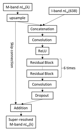
Figure 1.
Architecture of the convolution neural network. ReLu, rectified linear unit.
As in Liu and Wang (2021) [16], we retrain five networks with one network for each M-band nLw(λ). Network training requires a large amount of data as a training dataset, but we do not have 375 m resolution nLw(λ) data as ground truth. Therefore, we need to make an assumption that super-resolving nLw(λ) images from 750 m to 375 m resolution (original scale) is self-similar to super-resolving images on a degraded 1500 m to 750 m scale [16,51]. With this assumption, we train the networks on a degraded 1500 m to 750 m scale, i.e., VIIRS M-band nLw(λ) images are synthetically downsampled from 750 m to 1500 m, and used as coarse-resolution inputs, and the original images are treated as the ground truth. The networks trained with synthetic data have been proven to work well to super-resolve nLw(λ) images on the original scale [16]. Forty-five granules of VIIRS ocean color EDR data (Table 1) are used as the training dataset, and they are preprocessed into small patches of 32 × 32 pixels. We use 90% of patches for training the model weights and 10% for validation. The network and training are implemented in the Keras frameworks (https://github.com/keras-team/keras, accessed on 14 May 2021) with TensorFlow as backend.

Table 1.
List of Visible Infrared Imaging Radiometer Suite (VIIRS) environmental data record (EDR) granules of the Bohai Sea, Baltic Sea, and La Plata River Estuary used for training the network.
3. Results
3.1. Training Networks
The performance of the deep CNN relies heavily on the training datasets. VIIRS ocean color data over the Bohai Sea and Baltic Sea were used to train the networks for super-resolution of coastal ocean color images [16]. The maximum Kd(490) values of the Bohai Sea and Baltic Sea are usually ~2.0 m−1 and ~4.0 m−1, respectively. However, in extremely turbid coastal and inland lake regions, for example, the La Plata River Estuary [53], Kd(490) values can reach up to ~6.0–7.0 m−1 [54]. Therefore, super-resolution networks trained with the Bohai Sea and Baltic Sea data could not be able to accurately super-resolve nLw(λ) images over extremely turbid waters. We have to re-train the CNNs by also including nLw(λ) spectra data from highly turbid water regions such as La Plata River Estuary in the training datasets.
Forty-five granules (Table 1) of VIIRS-SNPP ocean color data from the Bohai Sea, Baltic Sea, and La Plata River Estuary were used to re-train five networks (one for nLw(λ) at each M-band), and they are referred to as networks with new training. In comparison, the networks trained previously with only the Bohai Sea and Baltic Sea data [16] are referred to as old training. The difference between the new training and old training is only in the training dataset, while the CNN model and the settings are kept the same. It is noted that the ocean color satellite images contain lots of missing data owing to clouds, high sun glint, high sensor-zenith angle, and so on. In our treatment of the missing data in the process of CNN, we assign the mean of all valid pixels in the images to all missing data points.
Figure 2 shows the comparison of the original images (750 m resolution) with super-resolved images (375 m resolution) of both old training and new training for nLw(443), nLw(551), and nLw(671), as well as Kd(490) and Chl-a on 27 February 2020, in the La Plata River Estuary. It can be seen that, for nLw(443) and nLw(671), the original images are essentially the same as the super-revolved images with both old training and new training. However, for nLw(551), the radiances with old training (Figure 2g) are obviously underestimated in the La Plata River Estuary (color looks more orange), while the data from new training (Figure 2l) are significantly improved and look very similar to the original image. As the training dataset of old training contains only data from the Bohai Sea and Baltic Sea, the networks of old training do not have the skills to super-resolve the images of highly turbid water regions. Consequently, Chl-a data are underestimated with old training (the color looks more greenish in the La Plata River Estuary in Figure 2j), as Chl-a are derived from nLw(443), nLw(486), and nLw(551) [7]. The training dataset of new training includes the data from the extremely turbid La Plata River Estuary, so Chl-a are significantly improved (Figure 2o). On the other hand, Kd(490) data are more correlated to nLw(671) [9], so the differences between using old training and new training are generally small (Figure 2i,n).
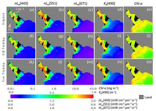
Figure 2.
Visible Infrared Imaging Radiometer Suite (VIIRS)-derived original images (a–e), super-resolved images with old training (f–j), and super-resolved images with new training (k–o) of nLw(443), nLw(551), nLw(671), Kd(490), and Chl-a in the La Plata River Estuary on 27 February 2020. Note that a line A is marked in Figure 2a for further analysis.
To quantitatively evaluate the difference between the results of using old training and new training, Figure 3 shows the line plots of nLw(443), nLw(551), nLw(671), Kd(490), and Chl-a along line A (pink line) marked in Figure 2a. As we can see in Figure 3, nLw(671) values are ~7.0 mW cm−2 μm−1 sr−1 (Figure 3a) and Kd(490) are generally ~6.0 m−1 (Figure 3b), which indicate that the region is indeed extremely turbid in the La Plata River Estuary [54]. In addition, nLw(551) values are also abnormally high (~5.0 mW cm−2 μm−1 sr−1), and they are higher than those in the Bohai Sea and Baltic Sea (~4.0 mW cm−2 μm−1 sr−1) [16]. Therefore, the networks trained in the Bohai Sea and Baltic Sea (old training) underestimate nLw(551) by ~7% in the La Plata River Estuary. Figure 3c and d shows the percent difference, i.e., 100 × (super-resolved − original)/original, of Chl-a and Kd(490) with old training (blue cross) and new training (red circle) along line A noted in Figure 2a. As a result, Chl-a concentrations are underestimated by ~21% with old training (Figure 3c), while Kd(490) are only underestimated by ~1% with old training (Figure 3d). With new training, both Kd(490) and Chl-a values are significantly improved with essentially zero biases. Therefore, it is concluded that including the data from highly turbid water regions in the training dataset (i.e., covering all possible data ranges) is necessary for the network models to accurately super-resolve satellite-measured Kd(490) and Chl-a images in various coastal and inland water environments.
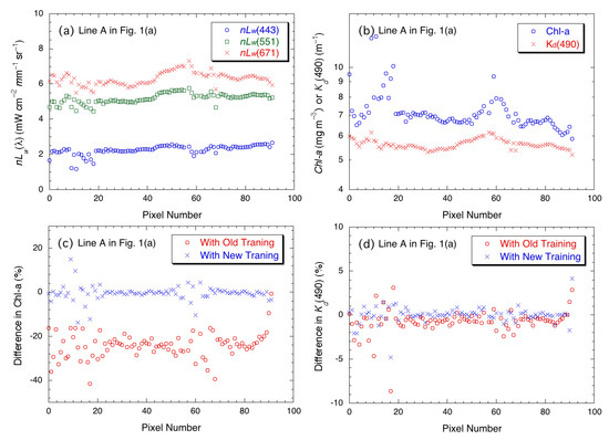
Figure 3.
Line plots (along line A in Figure 2a) for (a) nLw(443), nLw(551), and nLw(671); (b) Kd(490) and Chl-a; (c) percent difference of Chl-a with old training (blue cross) and new training (red circle); and (d) percent difference of Kd(490) with old training (blue cross) and new training (red circle).
3.2. Network Validation
As described in the previous section, the network training assumes that super-resolving nLw(λ) images from 750 m to 375 m resolution are self-similar to super-resolving images on a degraded 1500 m to 750 m scale. This assumption requires that the nLw(λ) relationships between bands of different spatial resolutions are self-similar within the relevant scale range, i.e., the transfer of spatial details in nLw(λ) from high-spatial resolution to low-spatial resolution bands does not depend on the spatial resolution itself, but depends only on the relative resolution difference. In fact, the assumption is supported by the literature on self-similarity in image analysis [55,56], and has been proven to be effective in image super-resolution applications [16,51]. Following the same validation procedure by Liu and Wang (2021) [16], quantitative evaluations of the networks of new training are performed by super-resolving nLw(λ) images on a degraded 1500 m to 750 m scale, and the original 750 m spatial resolution nLw(λ) data are treated as ground truth to evaluate the super-resolved nLw(λ) images. The networks obtained from new training are applied on down-sampled 1500 m resolution images in the Baltic Sea (Granule V2015226105214), Bohai Sea (Granule V2019105051208), and La Plata River Estuary (Granule V2020058172016), and the super-resolved 750-m-resolution data are compared pixel-by-pixel with the original nLw(λ) images for validation. The results show that the mean, median, and standard deviation (STD) of the super-resolved/original nLw(λ) ratio in the three regions on average are 0.995, 0.997, and 0.056, respectively. Therefore, the performance is consistent with the validation results tested previously in the Baltic Sea and Bohai Sea [16].
As the goal of this study is to super-resolve Kd(490) and Chl-a images, we also evaluate the performance of the networks on Kd(490) and Chl-a data on a degraded 1500 m to 750 m scale. Specifically, super-resolved 750 m nLw(λ) data generated above from the down-sampled 1500 m resolution are used to calculate Kd(490) and Chl-a data (super-resolved). Pixel-by-pixel comparisons between the super-resolved and original Kd(490) and Chl-a data of the same resolution are evaluated. The results show that the mean, median, and STD of the super-resolved/original Kd(490) ratio in the three regions on average are 1.003, 1.001, and 0.077, respectively. For Chl-a, the mean, median, and STD of the super-resolved/original ratio in the three regions on average are 0.995, 0.998, and 0.096, respectively. For both parameters, the biases between the super-resolved and original data are quite small, but their STD values are larger than those in nLw(λ). In addition, the performance of super-resolved Kd(490) and Chl-a in the La Plata River Estuary shows no significant difference than that in the Baltic Sea and Bohai Sea.
3.3. Super-Resolved Kd(490) and Chl-a in the Baltic Sea
The networks with new training are used to super-resolve to VIIRS M-band nLw(λ) images at the Baltic Sea from the spatial resolution of 750 m to 375 m. As the Baltic Sea is not a highly turbid region, the difference between using new training and old training can be neglected. The super-resolved nLw(λ) images of the VIIRS five M-bands in the Baltic Sea have been evaluated in the previous study [16]. In this study, we mainly focus on high-resolution Kd(490) and Chl-a products, which are derived from the super-resolved nLw(λ) spectra. Figure 4 shows the original Kd(490) and Chl-a images and super-resolved images of an EDR granule acquired on 14 August 2015 (Granule V2015226105214) in the Baltic Sea. It can be seen that the super-resolved Kd(490) image (Figure 4b) is much sharper than the original one (Figure 4a), and has more detailed fine spatial structures. For example, the green color filaments of high Kd(490) crossing line B (purple line) marked in Figure 4a look blurry (750 m spatial resolution), while those filaments are sharpened with clearer edges in Figure 4b (375 m spatial resolution). In addition, the fuzzy features on the side of the n-shape structure to the left end of line B in Figure 4a are replaced with many clear finer features in Figure 4b. Similar changes can be seen in other locations of the Kd(490) image. Some of the thick and blurry features in the original image are enhanced with two or more separated filaments in the super-resolved image, while some other very faint features in the original Kd(490) image are clearly highlighted with sharp lines in the super-resolved Kd(490) image. However, it should be noted that the general pattern and color of those features are the same in Figure 4a,b, which shows that the super-resolution process does not change the mean value of those features.
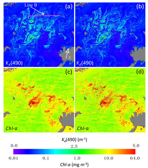
Figure 4.
Comparisons of ocean color images of the Baltic Sea on 14 August 2015, for (a) original Kd(490), (b) super-resolved Kd(490), (c) original Chl-a, and (d) super-resolved Chl-a. Note that line B is marked in Figure 4a for further analysis.
Similarly, fine spatial structures of Chl-a are also enhanced in the super-resolved images (Figure 4c,d). Because the Chl-a algorithm uses nLw(λ) at the blue and green bands, which is less correlated to nLw(638) [16], the pattern of the Chl-a features looks different from those of Kd(490) (as expected for the two different products). The high-concentration Chl-a filaments (yellow and red) are much sharper and thinner in the super-resolved image (Figure 4d), and some of the finer features that are not available in the original Chl-a image now appear in the super-resolved Chl-a image. As shown in Kd(490) images, the super-resolving process does not change the mean value of these Chl-a features, so the color of these Chl-a features is generally the same in the super-resolved and original images.
The enhancement of the super-resolved Kd(490) images is further evaluated quantitatively at the pixel level. Figure 5 shows the line plots of the super-resolved and original Kd(490) images along line B (pink line in Figure 4a). The original and super-resolved Kd(490) values are compared to nLw(638) along the line to demonstrate the performance of the network. The differences between Kd(490) and nLw(638) are usually quite large in magnitude in the Baltic Sea. However, we mostly care about the Kd(490) changes along line B for the purpose of performance evaluation. Therefore, we normalized nLw(638) and Kd(490) values along line B to the value of the first point on the left (by taking the ratio), so that we can easily compare their variations along the line. Figure 5a shows the line plots of the original and super-resolved normalized Kd(490) values along line B, as well as the normalized nLw(638) values on the same line (scale noted in the right). It can be seen that the super-resolved (normalized) Kd(490) images (red line) have more high-frequency variations than the original (normalized) Kd(490) images (blue line). These high-frequency variations correspond to the fine spatial features in the super-resolved Kd(490) images. It is also noted that the high-frequency (normalized) Kd(490) variations are mostly consistent with those in nLw(638) (green line). In fact, the high correlation coefficient of 0.9661 between super-resolved Kd(490) and nLw(638) indicates that the high-frequency variations in Kd(490) have been successfully transferred from the super-resolved M-band, which essentially learned from the I1 band (nLw(638)).
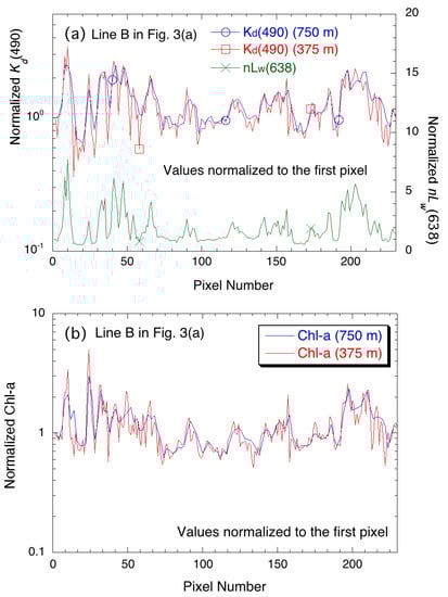
Similarly, Figure 5b shows line plots of the original and super-resolved Chl-a values (normalized) along line B. As shown in the Kd(490) results, there are more high-frequency variations in the super-resolved Chl-a line plot (red) than in the original one (blue). Compared with the super-resolved Kd(490), the super-resolved Chl-a is less correlated with nLw(638) (correlation coefficient of 0.6283). It can be seen that, although the low-frequency variations of Chl-a are not in line with nLw(638) (green line in Figure 5a), the network can still add high-frequency variations on top of low-frequency variations in the super-resolved Chl-a image.
Furthermore, we quantitatively compare the original Kd(490) and Chl-a images with the super-resolved images in the Baltic Sea. As each pixel in the original image corresponds to four pixels in the super-resolved image, the density-scatter plots of the super-resolved images versus original images by corresponding pixels for Kd(490) and Chl-a are shown in Figure 6, and they are both very close to the 1:1 line. The statistics of the ratio between the original Kd(490) (or Chl-a) images and the corresponding super-resolved images are also calculated. The mean ratios of the super-resolved/original Kd(490) and Chl-a image are 0.997 and 1.008, respectively, indicating that the biases between the original Kd(490) (or Chl-a) images and the corresponding super-resolved images are very small (<~1%). The STD values of the super-resolved/original image ratios for Kd(490) and Chl-a are 0.045 and 0.062, respectively. In fact, these variations are mostly caused by the added high-resolution features in the super-resolved Kd(490) and Chl-a images.
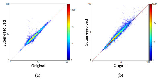
Figure 6.
Scatter-density plots of the super-resolved versus original images of (a) Kd(490) and (b) Chl-a in the Baltic Sea on 14 August 2015.
3.4. Tests in Other Coastal and Inland Waters
The performance of the networks is also tested in four coastal and inland water regions, i.e., the Bohai Sea, Chesapeake Bay, Lake Erie, and Gulf of Mexico, which include both sediment-dominate and phytoplankton-dominate waters. The networks with new training are applied to VIIRS ocean color data in the four regions to super-resolve nLw(λ) images of five M-bands, and then high-resolution Kd(490) and Chl-a are derived from the super-resolved nLw(λ) spectra for evaluations.
3.4.1. The Bohai Sea Region
The Bohai Sea is a major marginal sea of approximately 78,000 km2 on the east coast of China. In the Bohai Sea, the ocean dynamics and water properties are dominated primarily by river runoff, semidiurnal/diurnal tides, and seasonal monsoons, and so on [57]. As the Yellow River flows into the Bohai Sea, both sediments and phytoplankton blooms have significant effects on the water optical property in this region [58]. Shi et al. (2011) [59] also reported that the spring-neap tide can make significant Kd(490) variations in the Bohai Sea, as the tidal current plays an important role on sediment resuspension. In addition, the Kd(490) features can also be enhanced by the sand ridges on the bottom of the eastern Bohai Sea [58]. Figure 7 shows Kd(490) and Chl-a images in the Bohai Sea on 9 September 2018, as well as the ratio of the super-resolved/original image. Kd(490) data have a large dynamic range in the region, as its maximum value can reach as high as ~4 m−1 (Figure 7a). With the strong influence of the tidal current and wind waves [59], there are lots of fine dynamic features in satellite ocean color images. For example, the finger-shaped features on the bottom of the Kd(490) image are induced by the sand ridges on the ocean floor [60]. These features are significantly enhanced by the super-resolved Kd(490) image. To compare the original Kd(490) images with the super-resolved images, we calculate the pixel-by-pixel super-resolved/original Kd(490) ratio (Figure 7b). It can be seen in most parts of the image where Kd(490) are uniform, and ratios of super-resolved/original are close to 1.0 (green color). In the locations with some significant Kd(490) features, ratios of super-resolved/original deviate from 1.0. For example, the edges of the finger-shaped feature induced by sand ridges [60] are clearly modified, so that the feature edges are sharpened in the super-resolved image. The mean and STD of the super-resolved/original Kd(490) ratio for the region are 1.003 and 0.056, respectively (Table 2), which indicate that there are little biases between the super-resolved and original image. The Chl-a image of the Bohai Sea looks quite uniform (Figure 7c). Consequently, there is less enhancement in the super-resolved Chl-a image (Figure 7d). The mean and STD of the super-resolved/original Chl-a ratio for the region are 0.999 and 0.060, respectively.
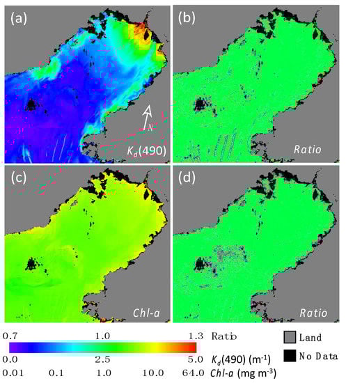
Figure 7.
(a) Original Kd(490), (b) ratio of super-resolved/original Kd(490), (c) original Chl-a, and (d) ratio of super-resolved/original Chl-a for a case in the Bohai Sea on 9 September 2018.
Table 2.
The statistics of the super-resolved/original ratio for Kd(490) and Chl-a in the Bohai Sea, Chesapeake Bay, Lake Erie, and Gulf of Mexico.
3.4.2. The Chesapeake Bay Region
The Chesapeake Bay is the largest estuary in the United States, and one of the most productive water bodies in the world. There are about 150 rivers, creeks, and streams flowing into the Chesapeake Bay, and the top five largest rivers, Susquehanna, Potomac, Rappahannock, York, and James rivers, contribute ~90% of discharge. As a large amount of freshwater (~2300 m3 s−1 on average) is discharged into the Chesapeake Bay, the dissolved and particulate materials can have a significant effect on the water property [61], and strongly influences phytoplankton production in the bay [48]. In addition, tidal forcing also plays an important role in sediment, biological, and geological processes in the Chesapeake Bay [62]. The upper Chesapeake Bay is extremely turbid because of the estuarine turbidity maximum (ETM) of the Susquehanna River [9,63]. Figure 8 shows Kd(490) and Chl-a images acquired on 3 March 2018, Granule V2018062175339, as well as the ratio of the super-resolved/original image in the Chesapeake Bay. It is noted that the Kd(490) value is so high (~5 m−1) in the upper Chesapeake Bay (Figure 8a) that, with old training, nLw(551) data are usually underestimated by ~4%, and Chl-a are generally underestimated by ~9%. The networks with new training work quite well; the super-resolved/original ratios for Kd(490) (Figure 8b) and Chl-a (Figure 8d) are both close to 1.0 (green color) in the upper Chesapeake Bay. Figure 8a also shows lots of Kd(490) features in the main stem of the Chesapeake Bay as well as in the tributaries. In general, it is much more turbid in the tributaries than in the main stem, as shown in Figure 8a. In the middle Chesapeake Bay, Kd(490) has the minimum in the center of the main stem, and gradually increases to the east and west shorelines. The super-resolution of all these water turbidity features is very important for routine monitoring of the Chesapeake Bay environment. It can be seen in Figure 8b that the super-resolution process is performed on these features with a significant Kd(490) gradient all around the Chesapeake Bay and the tributaries. On the other hand, Chl-a are generally uniform except in the middle bay region where the phytoplankton bloom is found on the west side of the Chesapeake Bay (Figure 8c). The super-resolution of the Chl-a is mainly performed in the middle bay (Figure 8d). In fact, as shown in Table 2, the mean values of the super-resolved/original ratios in Kd(490) and Chl-a are 1.010 and 1.004, respectively.
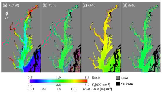
Figure 8.
(a) Original Kd(490), (b) ratio of super-resolved/original Kd(490), (c) original Chl-a, and (d) ratio of super-resolved/original Chl-a for a case in the Chesapeake Bay on 3 March 2018.
3.4.3. Lake Erie
Lake Erie, the southern most of the Great Lakes, is generally not extremely turbid (Kd(490) < ~3 m−1), except for the west side of the lake [64,65]. However, there are often significant water quality issues owing to rapid growth of algae, which is mainly caused by runoff of fertilizer and manure spread on large farm fields [66,67,68]. These problems not only threaten the lake’s ecosystem, but also the economic activities of the surrounding areas. Indeed, Lake Erie provides a primary drinking water source, and supports many recreational, tourism, and fishery activities. In addition, although most algae blooms in Lake Erie are harmless, the blue-green algae Microcystis produce toxins, and have harmful effects on human, birds, marine mammals, fish, and local economies [68,69]. Figure 9 shows Kd(490) and Chl-a images of Lake Erie on 29 April 2018 (Granule V2018119182603). There are some turbid features (Kd(490) > ~2.0 m−1) mainly on the west side of the lake, but for most area of the lake, waters are non-turbid (or relatively clear, Kd(490) < ~1.0 m−1) (Figure 9a). Figure 9b shows the super-resolved/original ratio of Kd(490) in Lake Erie. It can be seen that differences of the super-resolved and original Kd(490) images are small for most pixels, except for the feature edges. The Chl-a image looks quite uniform (Figure 9c), and there are less Chl-a feature enhancements than those in the super-resolution of Kd(490) image (Figure 9d). The mean values of the super-resolved/original ratio in Kd(490) and Chl-a are 0.998 and 0.995 (Table 2), indicating that the super-resolution process does not change the general values of the original Kd(490) and Chl-a images.
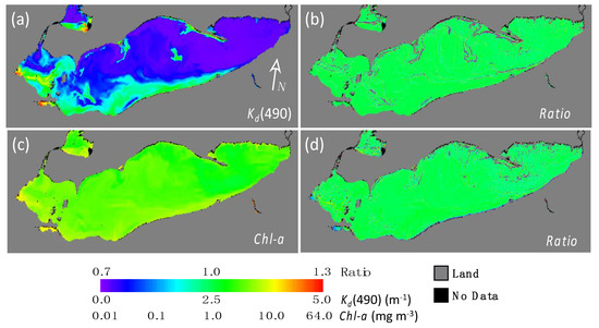
Figure 9.
(a) Original Kd(490), (b) ratio of super-resolved/original Kd(490), (c) original Chl-a, and (d) ratio of super-resolved/original Chl-a for a case in Lake Erie on 29 April 2018.
3.4.4. The Gulf of Mexico Region
As the fourth longest river in the world (~6300 km), the Mississippi River discharges at a speed of 18,400 m3 s−1 on average [70], and carries ~230 million tons of sediment into the Gulf of Mexico annually [71]. In the meantime, the Mississippi River brings a significant amount of nutrients into the Gulf of Mexico each year. As river plumes have significant effects on coastal marine ecosystems, including nutrient dynamics, biological productivity, water quality, and pollution hazards [72], high-resolution ocean color imageries can significantly benefit routine monitoring and understanding of river plume dynamics. Figure 10 shows the Kd(490) and Chl-a images of 19 November 2019 (Granule V2019323185429), which cover the turbid Mississippi River plume. As shown in Figure 10a, waters are usually highly turbid (Kd(490) > ~2.5 m−1) around the Mississippi River Delta, but the water is clear in the open ocean. There are some finer features on the boundary between the turbid and clear waters. Figure 10b also shows that there are significant super-resolution enhancements on the turbid–clear water boundaries, and on some coastal features as well. The Chl-a image provides similar features to those of Kd(490) around the Mississippi River Delta (Figure 10c), and the enhancement in the super-resolved image mainly occurs on the edge of these features. The mean values of the super-resolved/original ratios in Kd(490) and Chl-a are 1.002 and 1.015, respectively, in the Gulf of Mexico region (Table 2).
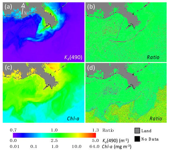
Figure 10.
(a) Original Kd(490), (b) ratio of super-resolved/original Kd(490), (c) original Chl-a, and (d) ratio of super-resolved/original Chl-a for a case in the Gulf of Mexico region on 19 November 2019.
In summary, from the results of the previous four examples, both Kd(490) and Chl-a images in the turbid coastal oceans and inland waters show many enhanced fine spatial features. While Chl-a images look relatively more uniform than Kd(490), significant super-resolution enhancements occur in both images. This is particularly useful for turbid coastal oceans and inland waters. In addition, super-resolution occurs mainly on pixels with significant Kd(490) and Chl-a spatial features, especially on the feature edges and locations with a large gradient. Overall, however, there are few differences on average between the original (750 m) Kd(490) and Chl-a images and the super-resolved (375 m) images in moderately and highly turbid coastal oceans and inland waters, showing that the super-resolution process does not change the mean values of the original ocean color product images.
4. Discussions and Conclusions
As satellite images from more sensors have become available, there are now many research activities dedicated to super-resolving remote sensing images. Liu and Wang (2021) [16] used the deep CNN to sharpen VIIRS M-band nLw(λ) images using the high-spatial resolution features from I1-band nLw(638) data. While nLw(λ) spectra of the five M-bands are primary parameters directly derived from VIIRS measurements, ocean/water biological and biogeochemical products Chl-a and Kd(490) are important water property data and have been widely used in the science and user communities for various research and applications [47,48,49,50]. In this study, we further develop and evaluate high-resolution Chl-a and Kd(490) products based on super-resolved VIIRS nLw(λ) images of the five M-bands. The deep CNN method is retrained with the training dataset from the Bohai Sea, Baltic Sea, and La Plata River Estuary as well, so that the performance of networks is significantly improved over extremely turbid coastal oceans and inland waters. In fact, the new trained networks, which cover wide water optical types, are generally applicable to various highly turbid coastal oceans and inland waters (other than the region with the training dataset). Indeed, the evaluation results show that a super-resolved Kd(490) image is much sharper than the original one, and has more detailed fine spatial structures. Although Chl-a features look different from Kd(490) (as expected), the fine spatial features are also enhanced in the super-resolved Chl-a images. The high Kd(490) and Chl-a filaments are much sharper and thinner in the super-resolved images, and some of the finer features that are not available in the original (750 m) images now appear in the super-resolved (375 m) images. The networks are also tested in four other coastal and inland waters. The evaluation results show that the super-resolution occurs mainly on pixels of Kd(490) and Chl-a spatial features (i.e., spatial variations), especially on the feature edges and locations with a large spatial gradient. It is also concluded that the super-resolution process does not change the mean value of the original images, while adding high-frequency features in the super-resolved water property product images.
It should be noted that the high-resolution Kd(490) and Chl-a images are derived from super-resolved nLw(λ) spectra images. As analyzed in Liu and Wang (2021) [16], the high-spatial resolution I1 band, nLw(638), is highly correlated to nLw(λ) of the VIIRS five M-bands, so that the networks are trained to extract high-frequency variations from nLw(λ) at the I1 band and transfer to those at M-bands. However, both Kd(490) and Chl-a algorithms use nLw(λ) at multi-spectral bands, and their relationships to that at the I1 band are not linear [7,9]. As can be seen in Figure 4, Kd(490) and Chl-a images usually show different patterns owing to differences in the algorithms, which indicate that they are not directly correlated. Thus, directly super-resolving Kd(490) and Chl-a images from coarse resolution to fine resolution is not as effective as that for nLw(λ). In fact, the evaluation results show that super-resolved nLw(λ) at the VIIRS five M-bands are quite accurate [16] and, consequently, VIIRS-derived Kd(490) and Chl-a images from super-resolved nLw(λ) spectra perform better than those from the direct super-resolution approach for Kd(490) and Chl-a.
It is also noted that the networks have the limitation when they are applied to super-resolve ocean color images in clear open ocean. Owing to the sensor characteristics, nLw(638) data generally have very weak signals with noticeable noise in the clear open ocean. Consequently, the networks add the data noise in the super-resolved nLw(λ), Kd(490), and Chl-a images. For example, in the open ocean outside of the Chesapeake Bay (Figure 8) and in the Gulf of Mexico (Figure 10), the value of Kd(490) is ~0.1 m−1, and the super-resolved Kd(490) and Chl-a images show some noise on the lower-right corner.
Because the performance of the deep CNN relies on the training dataset, it is recommended to verify and validate the super-resolved images when the networks are applied to other coastal and inland water regions, although the results show that the networks are also applicable to various coastal and inland water regions (different from the training dataset). Coastal and inland waters around the world generally show different optical properties owing to various suspended particulate matter types (e.g., sediment, phytoplankton, colored dissolved organic matter, and so on) as well as concentrations, which lead to complex M-band nLw(λ) spectra in VIIRS ocean color images. Abnormal nLw(λ) outside the range of the training dataset could result in inaccurate super-resolution in nLw(λ), Kd(490), and Chl-a images. The water turbidity seems to be an important factor that affects the super-resolution process. In our studies, the validation results indeed show that the networks with old training underestimate nLw(551) and Chl-a in the La Plata River Estuary and the upper Chesapeake Bay region. By including the La Plata River Estuary data in the training dataset (new training), it not only resolves the discrepancies in the La Plata River Estuary, but also in the highly turbid upper Chesapeake Bay region. Therefore, it is important to include various water types in the training dataset. We emphasize that it is not necessary to include all coastal/inland water data for the training, rather it is important to evaluate and validate the super-resolved images when the networks are applied to a new region of interest.
In the case of a discrepancy found between the super-resolved and original images when applied to a new region, network models need to be re-trained by including data of the region (or water type) in the training dataset. Fortunately, re-training the networks does not mean restarting from scratch. Instead, the networks can be trained incrementally, i.e., starting from the previously trained CNN weights, and re-training with only the new data. With this approach, the computation time to train with new dataset is significantly reduced, while the networks still retain all previously learned skills. By adding more and more data to the training dataset, the network model weights are gradually fine-tuned, and the network eventually will have the skills to super-resolve ocean color images of global coastal oceans and inland waters. Furthermore, we can also train the networks to utilize nLw(λ) spectra with high resolution images from many other satellite sensors. For example, OLCI on the Sentinel-3A/3B has spatial resolution of 300 m, and the Operational Land Imager (OLI) on Landsat-8 has spatial resolution of 30 m. In fact, the networks have the capability to simultaneously super-resolve high resolution ocean color data from multiple sources of different satellite sensors. Therefore, the high-spatial resolution imageries from multi-sensors and multi-bands can be fused into networks to conduct the super-resolving ocean color data processing.
Author Contributions
Conceptualization, X.L. and M.W.; methodology, X.L. and M.W.; software, X.L.; validation, X.L.; formal analysis, X.L. and M.W.; funding acquisition, M.W. All authors have read and agreed to the published version of the manuscript.
Funding
This research was supported by the Joint Polar Satellite System (JPSS) funding.
Acknowledgments
We thank three anonymous reviewers for their useful comments. The scientific results and conclusions, as well as any views or opinions expressed herein, are those of the author(s) and do not necessarily reflect those of NOAA or the Department of Commerce.
Conflicts of Interest
The authors declare no conflict of interest.
References
- Gordon, H.R.; Wang, M. Retrieval of water-leaving radiance and aerosol optical thickness over the oceans with seawifs: A preliminary algorithm. Appl. Opt. 1994, 33, 443–452. [Google Scholar] [CrossRef]
- IOCCG. Atmospheric correction for remotely-sensed ocean-colour products. In Reports of the International Ocean-Colour Coordinating Group; No., 10; Wang, M., Ed.; IOCCG: Dartmouth, NS, Canada, 2000. [Google Scholar] [CrossRef]
- Wang, M. Remote sensing of the ocean contributions from ultraviolet to near-infrared using the shortwave infrared bands: Simulations. Appl. Opt. 2007, 46, 1535–1547. [Google Scholar] [CrossRef]
- Wang, M.; Jiang, L. VIIRS-derived ocean color product using the imaging bands. Remote Sens. Environ. 2018, 206, 275–286. [Google Scholar] [CrossRef]
- O’Reilly, J.E.; Maritorena, S.; Mitchell, B.G.; Siegel, D.A.; Carder, K.L.; Garver, S.A.; Kahru, M.; McClain, C.R. Ocean color chlorophyll algorithms for SeaWiFS. J. Geophys. Res. 1998, 103, 24937–24953. [Google Scholar] [CrossRef]
- Hu, C.; Lee, Z.; Franz, B.A. Chlorophyll a algorithms for oligotrophic oceans: A novel approach based on three-band reflectance difference. J. Geophys. Res. 2012, 117, C01011. [Google Scholar] [CrossRef]
- Wang, M.; Son, S. VIIRS-derived chlorophyll-a using the ocean color index method. Remote Sens. Environ. 2016, 182, 141–149. [Google Scholar] [CrossRef]
- O’Reilly, J.E.; Werdell, P.J. Chlorophyll algorithms for ocean color sensors—OC4, OC5 & OC6. Remote Sens. Environ. 2019, 229, 32–47. [Google Scholar]
- Wang, M.; Son, S.; Harding, L.W., Jr. Retrieval of diffuse attenuation coefficient in the Chesapeake Bay and turbid ocean regions for satellite ocean color applications. J. Geophys. Res. 2009, 114, C10011. [Google Scholar] [CrossRef]
- Lee, Z.P.; Carder, K.L.; Arnone, R.A. Deriving inherent optical properties from water color: A multiple quasi-analytical algorithm for optically deep waters. Appl. Opt. 2002, 41, 5755–5772. [Google Scholar] [CrossRef]
- Shi, W.; Wang, M. A blended inherent optical property algorithm for global satellite ocean color observations. Limnol. Oceanogr. Methods 2019, 17, 377–394. [Google Scholar] [CrossRef]
- Werdell, P.J.; Franz, B.A.; Bailey, S.W.; Feldman, G.C.; Boss, E.; Brando, V.E.; Dowell, M.; Hirata, T.; Lavender, S.J.; Lee, Z.P.; et al. Generalized ocean color inversion model for retrieving marine inherent optical properties. Appl. Opt. 2013, 52, 2019–2037. [Google Scholar] [CrossRef]
- Wang, M.; Liu, X.; Tan, L.; Jiang, L.; Son, S.; Shi, W.; Rausch, K.; Voss, K. Impact of VIIRS SDR performance on ocean color products. J. Geophys. Res. Atmos. 2013, 118, 10347–10360. [Google Scholar] [CrossRef]
- Wang, M.; Isaacman, A.; Franz, B.A.; McClain, C.R. Ocean color optical property data derived from the Japanese Ocean Color and Temperature Scanner and the French Polarization and Directionality of the Earth’s Reflectances: A comparison study. Appl. Opt. 2002, 41, 974–990. [Google Scholar] [CrossRef]
- Goldberg, M.D.; Kilcoyne, H.; Cikanek, H.; Mehta, A. Joint Polar Satellite System: The United States next generation civilian polar-orbiting environmental satellite system. J. Geophys. Res. Atmos. 2013, 118, 13463–13475. [Google Scholar] [CrossRef]
- Liu, X.; Wang, M. Super-resolution of VIIRS-measured ocean color products using deep convolutional neural network. IEEE Trans. Geosci. Remote Sens. 2021, 59, 114–127. [Google Scholar] [CrossRef]
- Aiazzi, B.; Baronti, S.; Selva, M. Improving component substitution pansharpening through multivariate regression of MS + Pan data. IEEE Trans. Geosci. Remote Sens. 2007, 45, 3230–3239. [Google Scholar] [CrossRef]
- Atkinson, P.M. Issues of uncertainty in super-resolution mapping and their implications for the design of an inter-comparison study. Int. J. Remote Sens. 2009, 30, 5293–5308. [Google Scholar] [CrossRef]
- Choi, J.; Yu, K.; Kim, Y. A new adaptive component-substitution based satellite image fusion by using partial replacement. IEEE Trans. Geosci. Remote Sens. 2011, 49, 295–309. [Google Scholar] [CrossRef]
- Sales, M.H.R.; Souza, C.M.; Kyriakidis, P.C. Fusion of modis images using kriging with external drift. IEEE Trans. Geosci. Remote Sens. 2013, 51, 2250–2259. [Google Scholar] [CrossRef]
- Vivone, G.; Restaino, R.; Mura, M.D.; Licciardi, G.; Chanussot, J. Contrast and error-based fusion scheme for multispectral image pan-sharpening. IEEE Geosci. Remote Sens. Lett. 2014, 11, 930–934. [Google Scholar] [CrossRef]
- Wang, Q.; Shi, W.; Li, Z.; Atkinson, P.M. Fusion of Sentinel-2 images. Remote Sens. Environ. 2016, 187, 241–252. [Google Scholar] [CrossRef]
- Goodfellow, I.; Bengio, Y.; Courville, A. Deep Learning; MIT Press: Cambridge, MA, USA, 2016; Available online: http://www.deeplearningbook.org/ (accessed on 14 May 2021).
- Gordon, H.R.; Clark, D.K.; Mueller, J.L.; Hovis, W.A. Phytoplankton pigments from the Nimbus-7 Coastal Zone Color Scanner: Comparisons with surface measurements. Science 1980, 210, 63–66. [Google Scholar] [CrossRef]
- Hovis, W.A.; Clark, D.K.; Anderson, F.; Austin, R.W.; Wilson, W.H.; Baker, E.T.; Ball, D.; Gordon, H.R.; Mueller, J.L.; Sayed, S.T.E.; et al. Nimbus 7 Coastal Zone Color Scanner: System description and initial imagery. Science 1980, 210, 60–63. [Google Scholar] [CrossRef] [PubMed]
- McClain, C.R. A decade of satellite ocean color observations. Annu. Rev. Mar. Sci. 2009, 1, 19–42. [Google Scholar] [CrossRef]
- McClain, C.R.; Feldman, G.C.; Hooker, S.B. An overview of the SeaWiFS project and strategies for producing a climate research quality global ocean bio-optical time series. Deep Sea Res. Part II 2004, 51, 5–42. [Google Scholar] [CrossRef]
- Esaias, W.E.; Abbott, M.R.; Barton, I.; Brown, O.B.; Campbell, J.W.; Carder, K.L.; Clark, D.K.; Evans, R.L.; Hodge, F.E.; Gordon, H.R.; et al. An overview of MODIS capabilities for ocean science observations. IEEE Trans. Geosci. Remote Sens. 1998, 36, 1250–1265. [Google Scholar] [CrossRef]
- Salomonson, V.V.; Barnes, W.L.; Maymon, P.W.; Montgomery, H.E.; Ostrow, H. MODIS: Advanced facility instrument for studies of the earth as a system. IEEE Trans. Geosci. Remote Sens. 1989, 27, 145–153. [Google Scholar] [CrossRef]
- Rast, M.; Bezy, J.L.; Bruzzi, S. The ESA Medium Resolution Imaging Spectrometer MERIS a review of the instrument and its mission. Int. J. Remote Sens. 1999, 20, 1681–1702. [Google Scholar] [CrossRef]
- Donlon, C.; Berruti, B.; Buongiorno, A.; Ferreira, M.-H.; Femenias, P.; Frerick, J.; Goryl, P.; Klein, U.; Laur, H.; Mavrocordatos, C.; et al. The Global Monitoring for Environment and Security (GMES) Sentinel-3 mission. Remote Sens. Environ. 2012, 120, 37–57. [Google Scholar] [CrossRef]
- Tanaka, K.; Okamura, Y.; Amano, T.; Hiramatsu, M.; Shiratama, K. Development status of the Second-Generation Global Imager (SGLI) on GCOM-C. In Proceedings of the Sensors, Systems, and Next-Generation Satellites XIII, Berlin, Germany, 22 September 2009; Volume 7474. [Google Scholar]
- Shi, W.; Wang, M. An assessment of the black ocean pixel assumption for MODIS SWIR bands. Remote Sens. Environ. 2009, 113, 1587–1597. [Google Scholar] [CrossRef]
- Shi, W.; Wang, M. Characterization of global ocean turbidity from Moderate Resolution Imaging Spectroradiometer ocean color observations. J. Geophys. Res. 2010, 115, C11022. [Google Scholar] [CrossRef]
- Wang, M.; Liu, X.; Jiang, L.; Son, S. Visible Infrared Imaging Radiometer Suite Ocean Color Products. VIIRS Ocean Color Algorithm Theoretical Basis Document; NOAA/NESDIS/STAR: Maryland, USA, 2017. Available online: https://www.star.nesdis.noaa.gov/jpss/documents/ATBD/ATBD_OceanColor_v1.0.pdf (accessed on 14 May 2021).
- Jiang, L.; Wang, M. Improved near-infrared ocean reflectance correction algorithm for satellite ocean color data processing. Opt. Express 2014, 22, 21657–21678. [Google Scholar] [CrossRef]
- Wang, M.; Shi, W. The NIR-SWIR combined atmospheric correction approach for MODIS ocean color data processing. Opt. Express 2007, 15, 15722–15733. [Google Scholar] [CrossRef] [PubMed]
- Wang, M.; Shi, W. Estimation of ocean contribution at the MODIS near-infrared wavelengths along the east coast of the U.S.: Two case studies. Geophys. Res. Lett. 2005, 32, L13606. [Google Scholar] [CrossRef]
- Wang, M.; Son, S.; Shi, W. Evaluation of MODIS SWIR and NIR-SWIR atmospheric correction algorithm using SeaBASS data. Remote Sens. Environ. 2009, 113, 635–644. [Google Scholar] [CrossRef]
- Wang, M.; Tang, J.; Shi, W. MODIS-derived ocean color products along the China east coastal region. Geophy. Res. Lett. 2007, 34, L06611. [Google Scholar] [CrossRef]
- Wang, M.; Shi, W.; Tang, J. Water property monitoring and assessment for China’s inland Lake Taihu from MODIS-Aqua measurements. Remote Sens. Environ. 2011, 115, 841–854. [Google Scholar] [CrossRef]
- Morel, A.; Gentili, G. Diffuse reflectance of oceanic waters. III. Implication of bidirectionality for the remote-sensing problem. Appl. Opt. 1996, 35, 4850–4862. [Google Scholar] [CrossRef]
- Gordon, H.R. Normalized water-leaving radiance: Revisiting the influence of surface roughness. Appl. Opt. 2005, 44, 241–248. [Google Scholar] [CrossRef]
- Wang, M. Effects of ocean surface reflectance variation with solar elevation on normalized water-leaving radiance. Appl. Opt. 2006, 45, 4122–4128. [Google Scholar] [CrossRef] [PubMed]
- Wei, J.; Wang, M.; Lee, Z.; Briceño, H.O.; Yu, X.; Jiang, L.; Garcia, R.; Wang, J.; Luis, K. Shallow water bathymetry with multi-spectral satellite ocean color sensors: Leveraging temporal variation in image data. Remote Sens. Environ. 2020, 250, 112035. [Google Scholar] [CrossRef]
- IOCCG. Earth observations in support of global water quality monitoring. In Reports of International Ocean-Color Coordinating Group; No.17; Greb, S., Dekker, A., Binding, C., Eds.; IOCCG: Dartmouth, NS, Canada, 2018. [Google Scholar] [CrossRef]
- Behrenfeld, M.J.; Falkowski, P.G. Photosynthetic rates derived from satellite-based chlorophyll concentration. Limnol. Oceanogr. 1997, 42, 1–20. [Google Scholar] [CrossRef]
- Son, S.; Wang, M.; Harding, L.W., Jr. Satellite-measured net primary production in the Chesapeake Bay. Remote Sens. Environ. 2014, 144, 109–119. [Google Scholar] [CrossRef]
- Tomlinson, M.C.; Stumpf, R.P.; Ransibrahmanakul, V.; Truby, E.W.; Kirkpatrick, G.J.; Pederson, B.A.; Vargo, G.A.; Heil, C.A. Evaluation of the use of SeaWiFS imagery for detecting Karenia Brevis harmful algal blooms in the eastern Gulf of Mexico. Remote Sens. Environ. 2004, 91, 293–303. [Google Scholar] [CrossRef]
- Stumpf, R.P.; Culver, M.E.; Tester, P.A.; Kirkpatrick, G.J.; Pederson, B.; Tomlinson, M.C.; Truby, E.; Ransibrahmanakul, V.; Hughes, K.; Soracco, M. Use of satellite imagery and other data for monitoring Karenia Brevis blooms in the Gulf of Mexico. Harmful Algae 2003, 2, 147–160. [Google Scholar] [CrossRef]
- Lanaras, C.; Bioucas-Dias, J.; Galliani, S.; Baltsavias, E.; Schindler, K. Super-resolution of Ssentinel-2 images: Learning a globally applicable deep neural network. ISPRS J. Photogramm. Remote Sens. 2018, 146, 305–319. [Google Scholar] [CrossRef]
- He, K.; Zhang, X.; Ren, S.; Sun, J. Deep residual learning for image recognition. In Proceedings of the IEEE conference on computer vision and pattern Recognition (CVPR), Silver Spring, MD, USA, 27–30 June 2016; pp. 770–778. [Google Scholar]
- Dogliotti, A.I.; Ruddick, K.; Guerrero, R. Seasonal and inter-annual turbidity variability in the Rio de La Plata from 15 years of MODIS: El Nino dilution effect. Estuar. Coast. Shelf Sci. 2016, 182, 27–39. [Google Scholar] [CrossRef]
- Shi, W.; Wang, M. Water properties in the La Plata River Estuary from VIIRS observations. Continent. Shelf Res. 2020, 198, 104100. [Google Scholar] [CrossRef]
- Shechtman, E.; Irani, M. Matching local self-similarities across images and videos. In Proceedings of the IEEE Conference on Computer Vision and Pattern Recognition, Minneapolis, MN, USA, 17–22 June 2007. [Google Scholar] [CrossRef]
- Glasner, D.; Bagon, S.; Irani, M. Super-resolution from a single image. In Proceedings of the 2009 IEEE 12th International Conference on Computer Vision, Kyoto, Japan, 29 September–2 October 2009; pp. 349–356. [Google Scholar]
- Shi, W.; Wang, M. Ocean reflectance spectra at the red, near-infrared, and shortwave infrared from highly turbid waters: A study in the Bohai Sea, Yellow Sea, and East China Sea. Limnol. Oceanogr. 2014, 59, 427–444. [Google Scholar] [CrossRef]
- Shi, W.; Wang, M. Satellite views of the Bohai Sea, Yellow Sea, and East China Sea. Prog. Oceanogr. 2012, 104, 35–45. [Google Scholar] [CrossRef]
- Shi, W.; Wang, M.; Jiang, L. Spring-neap tidal effects on satellite ocean color observations in the Bohai Sea, Yellow Sea, and East China Sea. J. Geophys. Res. 2011, 116, C12032. [Google Scholar] [CrossRef]
- Shi, W.; Wang, M.; Li, X.; Pichel, W.G. Ocean sand ridge signatures in the Bohai Sea observed by satellite ocean color and synthetic aperture radar measurements. Remote Sens. Environ. 2011, 115, 1926–1934. [Google Scholar] [CrossRef]
- Schubel, J.R.; Pritchard, D.W. Responses of upper Chesapeake Bay to variations in discharge of the Susquehanna River. Estuaries 1986, 9, 236–249. [Google Scholar] [CrossRef]
- Shi, W.; Wang, M.; Jiang, L. Tidal effects on ecosystem variability in the Chesapeake Bay from MODIS-Aqua. Remote Sens. Environ. 2013, 138, 65–76. [Google Scholar] [CrossRef]
- Liu, X.; Wang, M. River runoff effect on the suspended sediment property in the upper Chesapeake Bay using MODIS observations and ROMS simulations. J. Geophys. Res. Oceans 2014, 119, 8646–8661. [Google Scholar] [CrossRef]
- Son, S.; Wang, M. Water quality properties derived from VIIRS measurements in the Great Lakes. Remote Sens. 2020, 12, 1605. [Google Scholar] [CrossRef]
- Son, S.; Wang, M. VIIRS-derived water turbidity in the Great Lakes. Remote Sens. 2019, 11, 1448. [Google Scholar] [CrossRef]
- Watson, S.B.; Miller, C.; Arhonditsis, G.; Boyer, G.L.; Carmichael, W.; Charlton, M.N.; Confesor, R.; Depew, D.C.; Hook, T.O.; Ludsin, S.A.; et al. The re-eutrophication of Lake Erie: Harmful algal blooms and hypoxia. Harmful Algae 2016, 56, 44–66. [Google Scholar] [CrossRef]
- Michalak, A.M.; Anderson, E.J.; Beletsky, D.; Boland, S.; Bosch, N.S.; Bridgeman, T.T.; Chaffin, J.D.; Cho, K.; Confesor, R.; Daloglu, I.; et al. Record-setting algal blooms in Lake Erie caused by agricultural and meteorological trends consisten with expected future conditions. Proc. Natl. Acad. Sci. USA 2013, 110, 6448–6452. [Google Scholar] [CrossRef]
- Steffen, M.M.; Belisle, S.; Watson, S.B.; Boyer, G.L.; Wilhelm, S.W. Status, causes and controls of cyanobacterial blooms in Lake Erie. J. Great Lakes Res. 2014, 40, 215–225. [Google Scholar] [CrossRef]
- Moore, T.S.; Mouw, C.B.; Sullivan, J.M.; Twardowski, M.S.; Burtner, A.M.; Ciochetto, A.B.; McFarland, M.N.; Nayak, A.R.; Paladino, D.; Stockley, N.D.; et al. Bio-optical properties of cyanobacteria blooms in western Lake Erie. Front. Mar. Sci. 2017, 4, 300. [Google Scholar] [CrossRef]
- Milliman, J.D.; Meade, R.H. World-wide delivery of river sediment to the oceans. J. Geol. 1983, 91, 1–21. [Google Scholar] [CrossRef]
- Meade, R.H.; Parker, R.S. Sediment in Rivers of the United States. In National Water Summary 1984; U.S. Geological Survey Water Supply Paper; U.S. Geological Survey: Reston, VA, USA, 1985; p. 49. [Google Scholar] [CrossRef]
- Shi, W.; Wang, M. Satellite observations of flood-driven Mississippi River plume in the spring of 2008. Geophy. Res. Lett. 2009, 36, L07607. [Google Scholar] [CrossRef]


Publisher’s Note: MDPI stays neutral with regard to jurisdictional claims in published maps and institutional affiliations. |
© 2021 by the authors. Licensee MDPI, Basel, Switzerland. This article is an open access article distributed under the terms and conditions of the Creative Commons Attribution (CC BY) license (https://creativecommons.org/licenses/by/4.0/).