Abstract
Stack emissions from the industrial sector are a subject of concern for air quality. However, the characterization of the stack emission plume properties from in situ observations remains a challenging task. This paper focuses on the characterization of the aerosol properties of a steel plant stack plume through the use of hyperspectral (HS) airborne remote sensing imagery. We propose a new method, based on the combination of HS airborne acquisition and surface reflectance imagery derived from the Sentinel-2 Multi-Spectral Instrument (MSI). The proposed method detects the plume footprint and estimates the surface reflectance under the plume, the aerosol optical thickness (AOT), and the modal radius of the plume. Hyperspectral surface reflectances are estimated using the coupled non-negative matrix factorization (CNMF) method combining HS and MSI data. The CNMF reduces the error associated with estimating the surface reflectance below the plume, particularly for heterogeneous classes. The AOT and modal radius are retrieved using an optimal estimation method (OEM), based on the forward model and allowing for uncertainties in the observations and in the model parameters. The a priori state vector is provided by a sequential method using the root mean square error (RMSE) metric, which outperforms the previously used cluster tuned matched filter (CTMF). The OEM degrees of freedom are then analysed, in order to refine the mask plume and to enhance the quality of the retrieval. The retrieved mean radii of aerosol particles in the plume is 0.125 m, with an uncertainty of 0.05 m. These results are close to the ultra-fine mode (modal radius around 0.1 m) observed from in situ measurements within metallurgical plant plumes from previous studies. The retrieved AOT values vary between 0.07 (near the source point) and 0.01, with uncertainties of 0.005 for the darkest surfaces and above 0.010 for the brightest surfaces.
1. Introduction
Human activities are responsible for significant emissions of particulate matter (PM). Atmospheric PM (also known as aerosols) is responsible for air quality degradation and the exposure of populations to ambient fine aerosols (PM), thus posing a global health concern [1,2]. The industrial sector was the second largest source of primary coarse aerosol (PM) emissions and the fourth largest source of PM in Europe between 2013 and 2018. According to the emissions inventory of the national emissions reported at the Convention on Long-range Transboundary Air Pollution [3], PM and PM from the industrial sector represented 15% and 6.5% of the total emissions in Europe over the period 2003–2018, respectively. Emission inventories can be generated from on-site measurements, modelling, and reporting by the industry sector. Industrial emissions depend on manufacturing processes, fuel, emission factors, and technological abatement. Industrial emission inventories are updated each year according to specific guidelines [4,5]. However, the temporal variability of instantaneous emission fluxes remains a challenge to assess; in particular, in the case of unexpected atmospheric emissions due to industrial accidents or uncontrolled releases.
Ground-level sensor networks, including remote sensing-based techniques, have been commonly used for fine particle monitoring [6]. Since the signing of the Convention of Long-range Transboundary Air Pollution in 1979, several monitoring programs have been deployed in Europe, such as the European Monitoring and Evaluation Programme (EMEP). However, such ground-based networks are not always able to appropriately capture the spatial dispersion of the plume from the emission source. Airborne and satellite remote sensing imagery may, therefore, be considered as complementary to ground-based systems.
The dilution of a stack plume in the ambient air depends on the wind field, the atmospheric stability [7], the effluent buoyancy, and momentum [8]. With dilution, the optical signature of the plume reduces in amplitude. Industrial plumes from an industrial stack generally have a rather limited visible spatial extent, only about a few hundred meters. Detecting a plume in a remote sensing image remains a challenge, and it is even more difficult to quantify the aerosol properties inside the plume. Hyperspectral visible/short-wave infrared (VIS-SWIR) imagery with a high spatial resolution (of about 1–10 m) is well-suited for the plume detection task and the study of aerosol properties [9,10,11]. Moreover, recent and planned high spectral and spatial resolution space missions have offered new opportunities for the study of stack emissions on a global scale.
Remote sensing of atmospheric aerosols has benefited from space missions dedicated to Earth observation (e.g., the NASA EOS program). First considered as a corrective parameter for estimating surface reflectances, aerosols have become an important focus of research, due to their important role in climate change. Kaufman and Sendra [12] and Kaufman et al. [13] have used the atmospheric correction approach for aerosol characterization over dark, densely vegetated pixels. This method is based on dedicated spectral channels or channel ratios of multi-spectral sensors and, since then, has been improved and successfully applied to multi-spectral images [14,15]. Variants of this method use channels with wavelengths below 500 nm over bright soils [16,17,18].
Inverse model analysis applied to aerosol satellite remote sensing is an ill-posed problem, for which statistical frameworks, such as optimal inversion [19,20,21,22,23], have been proposed. Thompson et al. [24,25] and Hou et al. [26,27] have presented a method based on the formalism of Rodgers [28], in order to simultaneously retrieve the atmospheric properties and the surface reflectance from VIS-SWIR images. Several studies have used the formalism of Rodgers to retrieve gas, aerosol, or surface properties from space missions such as SAGE II [21], IASI [29,30,31], and GOSAT [32]. Sequential algorithms, such as MAJA [33] or GRASP [34], allow for the retrieval of atmospheric properties with a multi-temporal comparison and a combination of several images. Sequential atmospheric correction algorithms have been used on hyperspectral data [35,36,37,38,39,40].
The retrieval of the aerosol optical properties of an industrial stack plume requires both surface and atmospheric correction. The plume properties can be estimated by using the difference between a reference image without the plume and the actual image with the plume. However, while atmospheric correction is usually homogeneous over the scene, the surface properties can be highly heterogeneous. Therefore, an adequate method is needed to infer the surface reflectance under the plume. The reference signal can be estimated from pixels out of the plume, through using a mean spectrum considering the class of surface reflectance [10] or by using multi-temporal data [11]. The method using the mean spectrum by class is appropriate for rather homogeneous classes. The reference can also be estimated from ancillary radiometric observations coming from other sensors, such as multi-spectral images, as is presented in this study.
In this paper, a method to improve the estimation of plume aerosol properties from hyperspectral image is described. The proposed framework is applied to a plume observed in February 2016 over a steel plant in France. The method is based on multi-temporal and multi-resolution observations, as well as an optimal estimation method (OEM). We first describe how the surface reflectance under the plume is determined, using either a single hyperspectral image or a combination of the hyperspectral and multi-spectral Sentinel-2 observations. The plume aerosol optical properties are first estimated using a sequential method and, then, an iterative optimal estimation method, taking into account the observations and forward model uncertainties.
2. Methods
2.1. Theory
A radiance signal measured by an airborne or satellite sensor on a flat, homogeneous, and Lambertian surface can be expressed [41] as:
where
L = at-sensor radiance in W·m−2·sr·m
= atmospheric radiance, without interactions with the ground
= direct part of the solar irradiance
= scattering part of the solar irradiance
= direct part of the atmospheric transmittance
= scattering part of the atmospheric transmittance
S = atmospheric spherical albedo
= surface reflectance of the studied pixel
= surface reflectance from the environment.
In the presence of a homogeneous semi-transparent plume between the sensor and the soil, , , , , and are modified. The total solar irradiance is given by , and the total atmospheric transmittance is given by . The pixel environment is assumed to be homogeneous, which means that is equivalent to . The surface reflectance, , is estimated by applying homogeneous atmospheric correction to the radiance image. The variational radiance signal due to the plume aerosols is modelled by:
where is the radiance signal measured for a single pixel in the same conditions as L, but with the presence of a plume, is the atmospheric radiance variation due to the plume aerosol, and is the variation of the product of the total irradiance with the total atmospheric transmittance. Philippets et al. [10] and Alakian et al. [42] have considered the plume as an infinite horizontal homogeneous layer. The plume is assumed to be here a finite horizontal homogeneous layer; this means that the direct part of the solar irradiance seen by a pixel under the plume may or may not pass through the plume. The variation of the scattering part of the solar irradiance seen by a pixel under the plume is a fraction of that seen in the case of an infinite plume layer. The total variation of the solar irradiance due to the plume and seen by a pixel can be expressed as follows:
where is equal to 0 or 1, is a scalar between 0 and 1, is the direct part of the total irradiance variation, and is the scattering part of the total irradiance variation in the case of an infinite plume layer. In the same way, the surface reflectance variation, , due to the plume aerosol is:
where is the surface reflectance impacted by the plume.
2.2. Definition of the Optimal Estimation Method
The retrieval method is based on the optimal estimation method defined by Rodgers [28]. The OEM problem can be straightforwardly represented by Equation (5). The measure y is explained through the forward model function, F, associated with the state vector x and a random noise . In this study, the state vector x corresponds to atmospheric and surface properties, while the forward model is a radiative transfer model.
In the linear case, the forward model can be expressed as , where K is the Jacobian matrix containing the partial derivatives corresponding to the sensitivities of the direct model to the state parameters. In this form, the problem is ill-posed, as there are more unknowns than observations. To reduce the number of unknowns, prior knowledge of the state vector is used. The optimization method consists of minimizing the cost function to a global minimum. According to Rodgers [28], the cost function is expressed by Equation (6):
where the first term of the equation represents the difference between the state vector x and the a priori state vector, given the a priori variance-covariance matrix ; while the second term represents the error between the forward model and the observations y, given the variance–covariance matrix of the observations . The variance–covariance matrices and represent the uncertainties of the observation and the a priori state vector, respectively. According to the formalism of Rodgers, can be decomposed into:
where is the variance–covariance matrix representing the uncertainties due to the sensor and represents the effects of unknowns; that is, parameters that have an impact on retrieval uncertainties but were not retrieved during the OEM processing. is the Jacobian matrix associated with the unknown parameters. Rodgers [28] theoretically defined an estimator of the state vector of the retrievals, as follows:
The Jacobian matrix is also defined as the pseudo-inverse of the gain matrix, G, which represents the sensitivity of the estimated state vector to the observations y. The gain matrix G is computed by the following expression:
The elements of G correspond to the partial derivatives of the estimated state vector , with respect to the observation y. The gain matrix gives access to the averaging kernel matrix . The diagonal elements of A represent the degrees of freedom (DOF) associated with the state parameters. The trace of A gives the total DOF of the problem (i.e., the number of independent parameters). Finally, the rows of A give the sensitivity of the retrieved parameters to the true state. In the case of a perfect estimate of x, the matrix A would be the identity matrix. The true error corresponding to a random measurement noise is defined by:
and the posterior distribution of the estimated parameters has a covariance matrix given by:
The uncertainty given by depends on the resolving error caused by the lack of resolution in the inverse process and measurement errors due to the measurement noise. The measurement error and resolving error covariance matrices are and , respectively, which are defined by:
2.3. Forward Model Definition and State Vectors
The forward radiance model, , is defined by the following equation:
where L (see Equation (1)) is the estimated radiance without the plume and (see Equation (2)) is the radiance differential due to the aerosol plume. The forward radiance model is estimated using the radiative transfer model with the following input parameters: Atmospheric background properties (water vapor, background aerosol properties), the finite plume geometry parameters (i.e., the direct and scattering parts of the irradiance differential, defined as and in Section 2.1), the aerosol plume refractive index , the plume modal radius r, the log-normal size distribution standard deviation , and the plume aerosol optical thickness (AOT) at 550 nm . We assume that is linear, with AOT in the range of [0, 0.5] [10].
where () represents the AOT ratio between a reference AOT at 550 nm and the observed AOT at 550 nm. The atmosphere modelling was performed with the COMANCHE software [43], a frontend of MODTRAN model version 5.2 [44]. The plume was modelled by a homogeneous layer with a defined vertical extent, a height above the ground level, and an aerosol optical thickness at 550 nm, defined by the user. The aerosol plume optical properties were simulated using Mie theory, considering a mono-modal size distribution for a given modal radius r, with an associated standard deviation set to 1.5. The simulations were performed for 3 different refractive indices , corresponding to sulphate, brown carbon, and soot particles (Table 1).

Table 1.
Complex aerosol refractive index at 550 nm used in the plume simulations.
The plume reference AOT was set to 0.1 at 550 nm (optically thin plume). The plume had a vertical extent of 100 m and was located 10 m above ground level. The vertical extent of the plume was within the common range of industrial stack plume extension [8]. Moreover, the plume reference AOT and vertical extent values have no impact on the retrieved plume properties, as long as the AOT value is less than 0.5 [10].
The state vector x is associated with the OEM retrieved parameters, with a prior distribution , and with a prior variance–covariance matrix . The state vector x includes: (i) The surface reflectance vector , (ii) the plume AOT at 550 nm , and (iii) the aerosol plume modal radius r. The prior distribution of the retrieved parameters and their variance–covariance matrix are given by:
Pixel-by-pixel estimation of the prior value is defined in the next section. The covariance matrix, , of the surface reflectance was computed class-by-class. The covariance matrix and were estimated from the standard deviation of the prior values and , respectively, and from the forward model sensitivity analysis (see Section 2.5).
The state vector b corresponds to the forward model inputs that are not retrieved by the OEM. The associated variance–covariance matrix, , represents the variance of the error of those unknown parameters. The state vector b includes the atmospheric water vapor content, background aerosol Ångström coefficient, and background atmospheric visibility. Visibility is related to ground surface aerosol extinction at 550 nm by the Koschmeider equation, and was used to scale the MODTRAN aerosol extinction profile.
2.4. Forward Model Initialization: First Guess
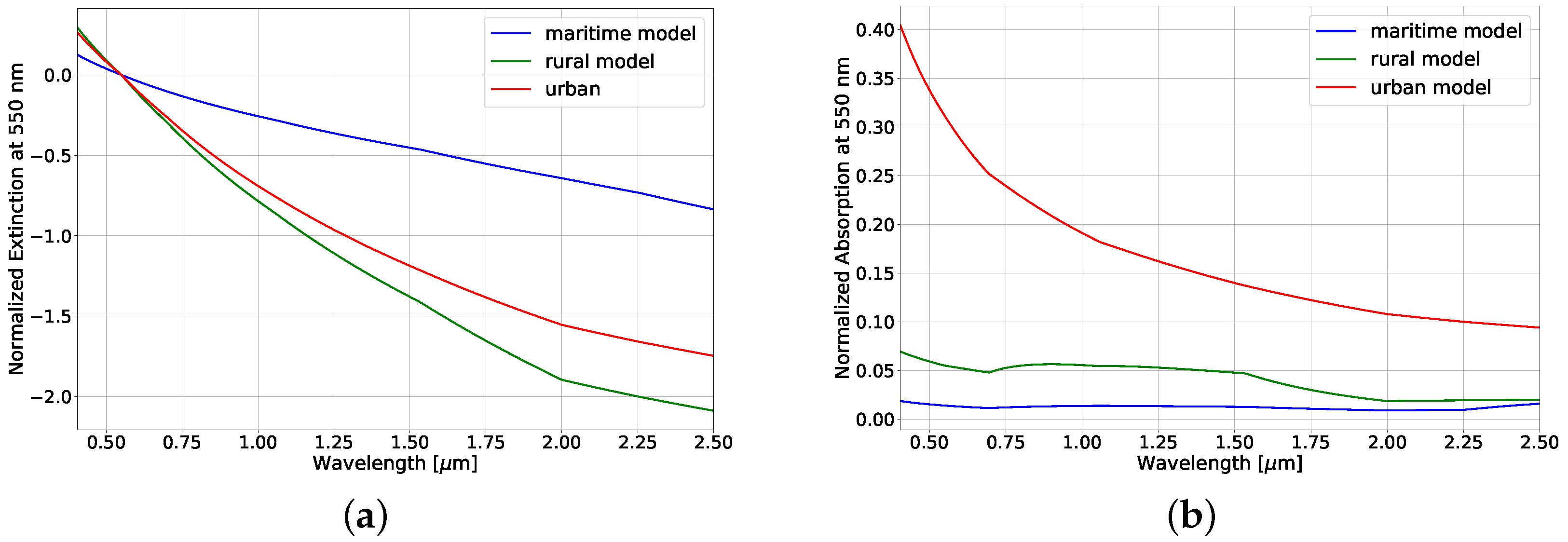
This step aims to initialize b and x and their associated uncertainties. Atmospheric background properties were estimated using MSI surface reflectances and the MODTRAN aerosol database. The MODTRAN background aerosol models were of three types: “maritime”, “rural”, or “urban”. The rural aerosol model was composed of a mixture of 70% water soluble substances and 30% dust-like aerosols. The urban aerosol model was a mixture of rural aerosol particles and soot-like aerosols produced by industrial activities. The proportions of rural aerosols and soot-like aerosols in the urban aerosol model were 80% and 20%, respectively. The maritime aerosol model was composed of sea-salt particles created by the evaporation of sea-spray droplets and of continental aerosols, which were almost identical to those of the rural model. The exception was that the largest particles in the rural aerosol model were removed. Each aerosol model was defined by the normalized extinction and absorption coefficients at 550 nm. Figure 1a,b presents the normalized extinction and absorption coefficients for each model.
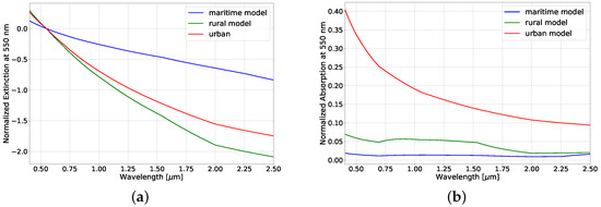
Figure 1.
Normalized (a) extinction and (b) absorption coefficients of MODTRAN background aerosol model.
The state vector b and the associated matrix were initialized at this stage. The water vapor uncertainty (see Section 4.1) was set to 10% of the initial concentration of the mid-latitude winter profile defined by MODTRAN. Channels above 920 nm that were strongly affected by water vapour were not considered. The visibility error was fixed at 15%, corresponding to an absolute error of 5 km (see Section 4.1). The error in the background aerosol model was defined using the Ångström coefficient Å [45]. The Ångström coefficients were 0.48, 1.32, and 1.15 for the “maritime”, “rural”, and “urban” aerosol models, respectively. The standard deviation of the error associated with the Ångström coefficients was set to 10%.
Surface reflectances were estimated by compensating for the atmospheric effects in the same way for the whole image, including the plume area. An extra step was needed to estimate the “off plume” surface reflectance in the plume area. In the case of a hyperspectral image alone, the “off plume” surface reflectance was assumed to be the estimated average spectrum, class-by-class. The images were classified with a random forest algorithm. The classification was performed with six user-defined classes: “water”, “sparse vegetation”, “dense vegetation”, “concrete soils”, “dark soils”, and “bright soils”. The training data sets were polygons drawn by the user using the open source geographical information system QGIS [46].
In the case of a single hyperspectral image associated with a multi-spectral image, different surface reflectance estimation methods may be considered. Different fusion algorithms exist, such as MAP-SMM [47] or FUSE [48], which are based on Bayesian approaches, or methods like Hysure [49], ICCV’15 [50], or CNMF [51], which are based on unmixing analyses. The coupled non-negative matrix factorization (CNMF) algorithm of Yokoya et al. [51] does not depend on image classification and the prior unmixing is unsupervised. CNMF merges a hyperspectral image with a multi-spectral image to obtain a final image, where each pixel is computed as a linear combination of the end members of the hyperspectral image. Vertex components analysis (VCA) [52] is used to obtain an initial set of endmembers for the hyperspectral image. The extracted hyperspectral endmembers and their weights are refined by alternating unmixing of hyperspectral and multi-spectral images by non-negative matrix factorization (NMF) [53,54]. Then, CNMF calculates the abundance matrix of hyperspectral endmember spectra using the multi-spectral image. The ground reflectance, (see Equation (16)), is then estimated, by combining the abundance matrix and the hyperspectral endmembers. The associated covariance matrix, , is then computed class-by-class.
First guesses of the AOTs and mean radii were estimated with a sequential approach based on the hyperspectral image corrected for the atmosphere. Atmospheres containing different types of plumes were simulated using the forward model. Three types of aerosol were considered (see Table 1). The standard deviation of the log-normal size distribution was equal to 1.5 and the modal radius varied from 0.025 m to 1 m. The sequential approach was performed using the surface reflectance differential defined in Equation (4), where is the prior reflectance estimated with the CNMF method and is the hyperspectral data corrected for the atmosphere. The reflectance differential was compared to the simulations , using the cluster-tuned matched filter (CTMF) or the root-mean-square error (RMSE) as a metric. The analysis of the metric scores led to a first pixel-by-pixel estimation of the optical thickness, aerosol type, and modal radius of plume particles.
CTMF was developed by Funk et al. [55] and is used to retrieve gas thermal signatures (CO, SO, NO, and O) in the thermal infrared. It was later adapted by Thorpe et al. [56,57] and Dennison et al. [58], in order to detect other gases in the reflective domain. Most recently, Philippets et al. [10] used CTMF to detect and characterize the aerosol signature of industrial plumes. The CTMF model can be described as a combination of the surface reflectance with the spectral reflectance signature of the plume aerosols . Both vectors and have the same dimension (i.e., the number of channels m in the hyperspectral image). After the classification of a hyperspectral image, an optimal filter for a soil class j can be defined as:
where represents the inverse of the correlation matrix of the soil class j and represents the mean aerosol spectral signature equivalent to . From the optimal filter associated to a modal radius and an aerosol type, the CTMF score, , describes the correlation between the simulated and the measured aerosol signal, which can be expressed as:
where is the optical thickness ratio between the true optical thickness and the reference optical thickness at 550 nm , which was fixed to 0.1 in the direct model. A CTMF score map was computed for each aerosol radius and type. As the aerosol type was assumed to be homogeneous inside the plume, the aerosol type associated to the most frequent best score inside the plume was chosen for the entire plume. Once the aerosol type was selected, a second application of the CTMF was performed. The radius map was computed by selecting the best CTMF score in the set of CTMF maps for each pixel. The AOT was then deduced, by comparing the estimated surface reflectance differential map with the simulated variation of the surface reflectance corresponding to the selected modal radius r pixel-by-pixel:
The RMSE defined by Equation (20) was used as an alternative metric to estimate the aerosol type, radius, and AOT.
where n is the number of channels of the spectrum and r is the modal radius. was computed, by Equation (4), for each pixel and for the different aerosol properties. Aerosol properties were set pixel-by-pixel to the minimum RMSE value.
2.5. Sensitivity Analysis
Retrieval uncertainties, in terms of modal radius and AOT, were due to: (i) The signal-to-noise ratio (SNR); (ii) the ground reflectance error (retrieved by the OEM); and (iii) parameters not retrieved by the OEM (forward model assumptions). The OEM non-retrieved parameters were the atmospheric background properties (b state vector), the finite plume geometry parameters (i.e., the direct and scattering parts of the irradiance differential, defined as and in Section 2.1), the aerosol plume refractive index , and the aerosol plume size distribution standard deviation .
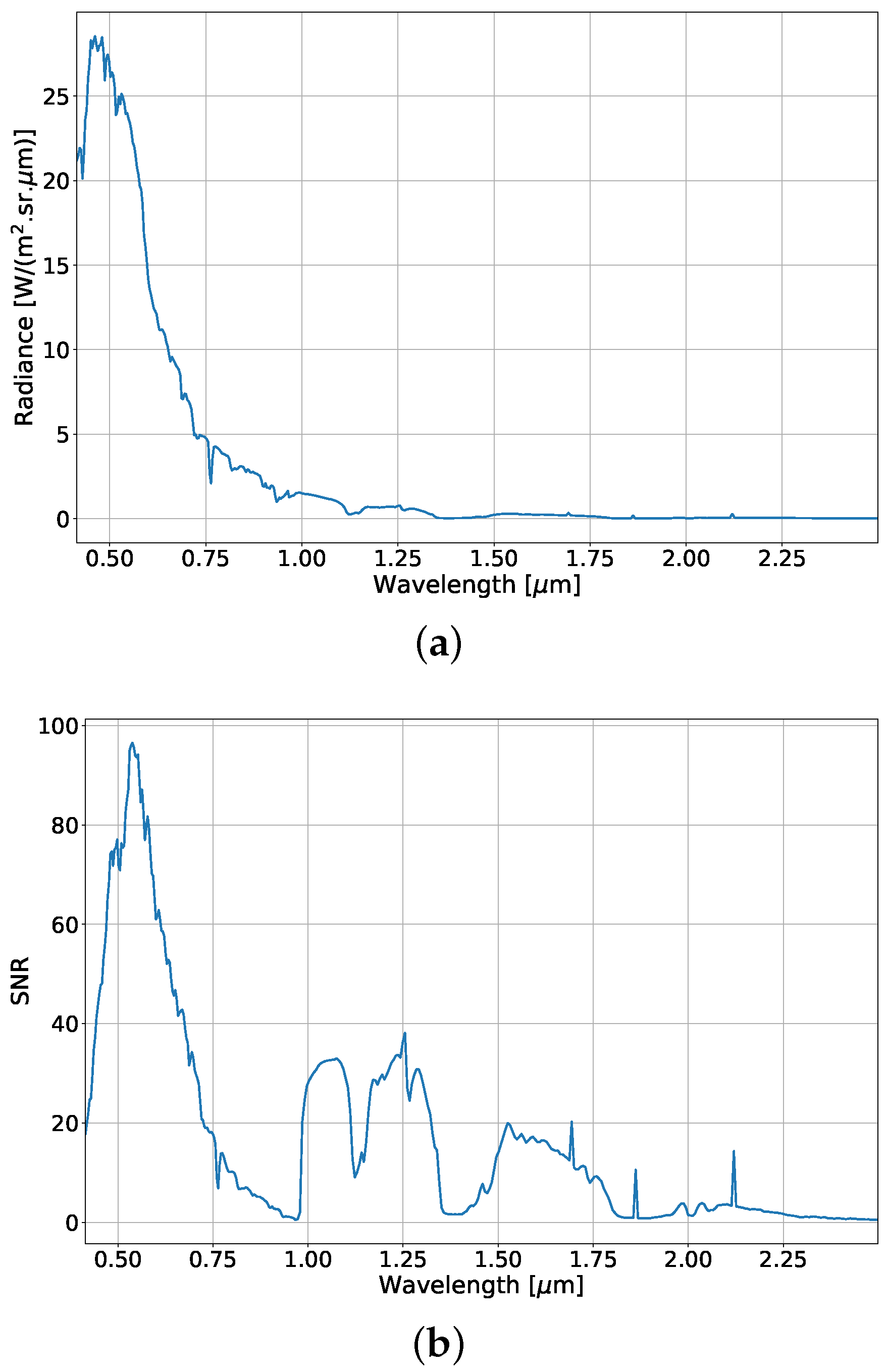
The instrument noise is a diagonal matrix with diagonal elements , representing the square of the noise equivalent delta radiance (NEDL). The NEDL was computed by , where represents the residual noise and represents the photonic noise. The coefficients and were given by the noise model of the HYSPEX sensor. Figure 2 represents the modelled SNR of the HYSPEX sensor for the mean radiance of water pixels.
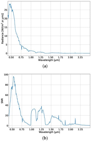
Figure 2.
Water pixel: (a) Mean radiance spectrum; and (b) associated signal-to-noise ratio.
The reference simulation state corresponded to seawater reflectance, a background aerosol model set to the MODTRAN rural mode with a visibility of 15 km. The scattering aerosol plume modal radius was set to 0.15 m and the AOT to 0.1, respectively. The coefficients and were set to 0.0 and 0.3, respectively. The reference state was closed to the observation case. From the reference state, we estimated the retrieval uncertainties due to a nominal variation (or uncertainty) of the forward model inputs or assumptions. Estimated retrieval uncertainties corresponding to the HYSPEX noise were around 0.0024 for AOT and 0.001 m for the modal radius.
Table 2 shows the modal radius and AOT retrieval uncertainties due to forward model input uncertainties. Parameter uncertainties were defined consistently with the data and the initialisation step (Section 2.4). The surface reflectance uncertainty was set to 10% and uncertainties corresponding to the water vapor, the background aerosol Ångström coefficient, and the visibility used in the forward model were set to 10%, 10%, and 15%, respectively. An uncertainty of 10% was set for the standard deviation of the plume aerosol size distribution. Then, an uncertainty of 10% was set for the value of the real part of its refractive index. The finite plume geometry parameter uncertainties were set to 0.2 for and to 1 for .

Table 2.
AOT and modal radius uncertainties corresponding to the uncertainties on the background aerosol model with the visibility and Ångström coefficient, the water vapor, the plume geometry and , the real part of the refractive index , the standard deviation of the plume aerosol size distribution, the surface reflectance relative error , and the surface reflectance offset.
We observed that most of the uncertainties due to the model assumption were higher than the measurement noise for both the AOT and modal radius. The maximum AOT error of 0.012 (i.e., a relative error of 12%) was due to a reflectance offset error: An error of 0.01 corresponds to more than 20% of water mean reflectance in the VIS spectral domain. As expected, the maximum modal radius error of 0.045 (i.e., a relative error of 30%) was due to uncertainty, as the retrieved modal radius is closely linked with the input size distribution standard deviation. The least sensitive parameters (errors with the same range of magnitude as noise error) were water vapor, for AOT, and and visibility for modal radius. In the case of other parameter uncertainties, retrieval error due to model uncertainties were quite similar, with a mean value around 0.005 (10%) for AOT and around 0.015 (10%) for modal radius. The forward model assumption uncertainties defined in this analysis led to acceptable uncertainties, in terms of the modal radius and AOT.
3. Data
3.1. Airborne Hyperspectral Data
A plume emitted by the stack of the sinter plant at the ArcelorMittal site was imaged by the HYSPEX hyperspectral camera aboard the SAFIRE ATR-42 research aircraft on the 17th of February at 11:00 LT. The ArcelorMittal site is located in the Fos-sur-Mer district area and is the second largest steel plant in France, which produces steel, coils, and tubes. According to the IREP database (Registre français des rejets et des transferts de polluants), the Fos-sur-Mer ArcelorMittal industrial site was, respectively, the first and the second emitter of (1230 t/year) and CO (7,460,000 t/year) for France in 2018. The HYSPEX camera has a spectral range between 0.41 and 2.5 m with 160 spectral channels in the visible/near-infrared (VNIR) range (410–996 nm) and 262 in the short-wave infrared (SWIR) range (970–2500 nm). The HYSPEX spatial resolution is 0.5 m × 1 m in the VNIR and 2 m × 2 m in the SWIR.
The georeferencing of the hyperspectral VNIR and SWIR images in UTM zone 31N was performed with QGIS, using a 50 cm spatial resolution ortho-rectified picture of the scene given by the Institut Géographique National (IGN) [59]. The georeferencing was performed with wedge points positioned manually on the IGN ortho-image. The VNIR image resolution was set to the SWIR resolution by using a spatial matching algorithm based on pixel matching through an optical flow calculation called GEFOLKI [60,61].
3.2. Sentinel-2 Products
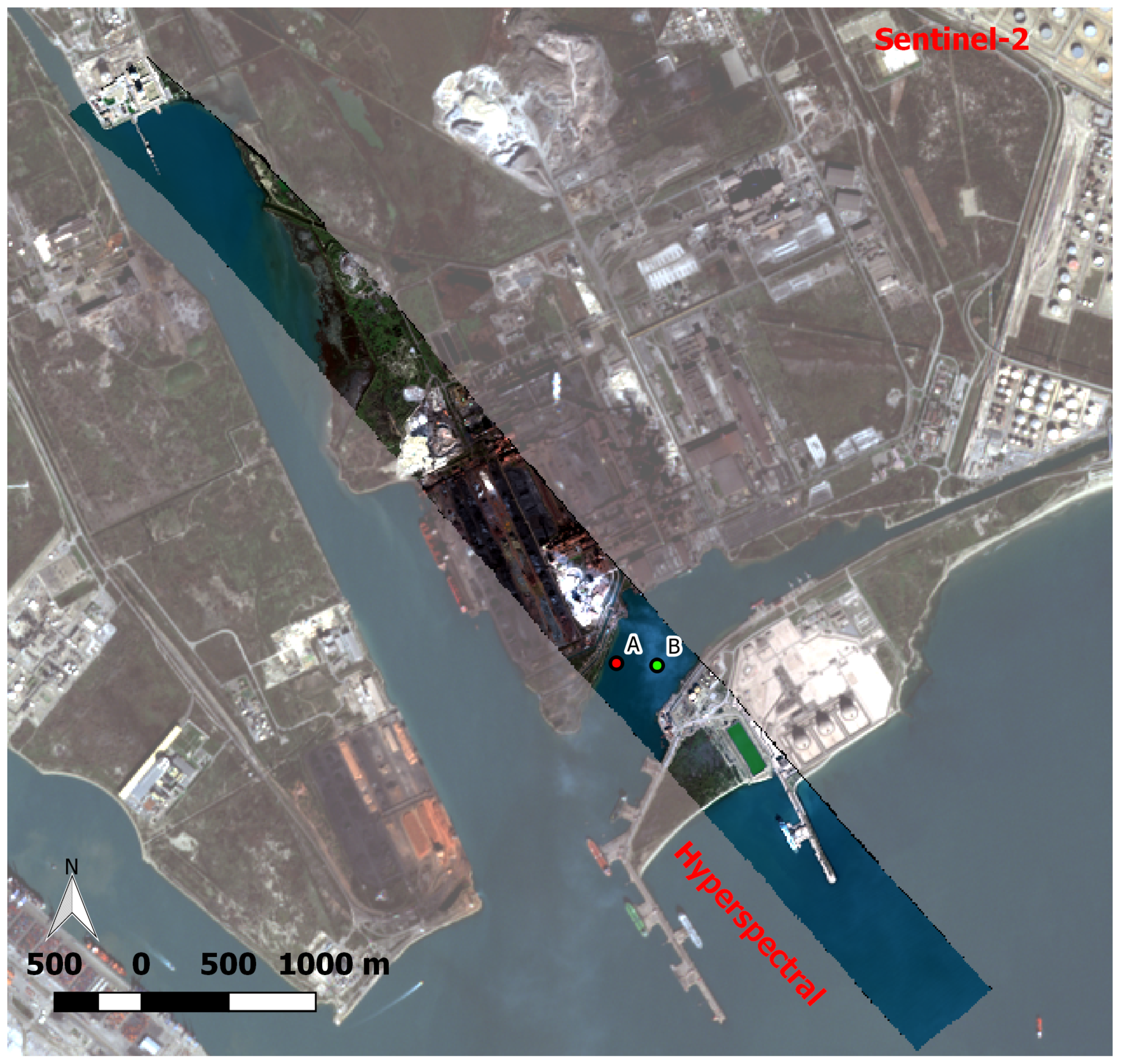
Sentinel-2 (S2) was first launched in June 2015 (first platform), and a second platform was launched in March 2017. Sentinel-2 is equipped with the multispectral instrument (MSI), which acquires Earth atmosphere-reflected radiances in 13 spectral bands ranging from 442 nm to 2202 nm. The spatial resolution of MSI ranges from 10 m to 60 m, depending on the spectral channel. We selected an MSI image acquired on the 5th of February, 2016, being the closest S2 acquisition date to our airborne acquisition. The MSI image was processed using the MAJA algorithm [33]. The MAJA algorithm performs a masking procedure to detect and remove clouds and their shadows from the Level 1C image. The surface reflectance was derived following the algorithm proposed by Hagolle et al. [62]. Hereinafter, we used the level 2A surface reflectance product delivered by the processing chain of the THEAI center [63]. We used the channels B2 to B12, except for B9 and B10. The spatial resolution was set to 10 m for the selected bands. A first atmospheric correction was performed on the HYSPEX image, in order to apply a spatial matching algorithm (GEFOLKI) between MSI and HYSPEX surface reflectances to produce geolocalized images at a spatial resolution of 10 m. The transformation matrix, computed by GEFOLKI spatial matching, was then applied to the HYSPEX radiance image. Figure 3 shows a superposition of an RGB composite image of the HYSPEX image on S2 over the studied area. The stack and associated plume are located in the center of the image. The plume moves south-east over a water channel, crosses a ground arm with wharves, and then moves over the sea. The scene is complex, with varying surface reflectances due to the presence of industries, water bodies, vegetation, and communication networks.

Figure 3.
HYSPEX hyperspectral image (opaque) superposed on the Sentinel-2 image (transparent). Points A and B, respectively, represent areas of interest for the spectra used in Figure 7.
4. Results
4.1. Atmospheric Correction
The optimal estimation procedure was applied to the off-plume pixels in the HYSPEX image, in order to estimate the atmospheric radiative terms. MSI surface reflectances were used to constrain the retrievals. However, MSI reflectances in the SWIR for water and dark vegetation were overcorrected, consequently leading to an overestimation of the visibility. SWIR channels had an influence on the OEM within the plume, as the uncertainty on the surface reflectance was very large. SWIR channels were, therefore, only used for the surface classification (see below), and not for plume retrieval. The most likely background aerosol models were the “maritime” and “rural” models, with a visibility of 18 ± 5 km and 15 ± 4 km, respectively. We selected the rural aerosol model for atmospheric correction. As mentioned in the method section, an error term on the aerosol model selection was introduced through use of the Ångstrom coefficient. The algorithm did not converge when using the urban background model, due to its much higher absorption coefficient (see Figure 1b).
4.2. Image Classification
Figure 4 shows the surface reflectance classification results using the random forest procedure applied to the HYSPEX and MSI images. One can notice that a large part of the plume remained visible over water when using a single hyperspectral datum, while it disappeared when using the combination of HYSPEX and MSI. Moreover, the hyperspectral classification was more heterogeneous and misclassified “bright soils” or “sparse vegetation”. As expected, the footprint of the plume was missing in the MSI classification. The classification of the MSI image was more homogeneous than that of HYSPEX; however, it over-classified spectra in the “concrete soils” class. This over-classification mainly concerns spectra that should have been classified as “bright soils”.

Figure 4.
Snapshots of Surface reflectances obtained from radiances acquired by HYSPEX camera; (A) surface classification using HYSPEX image alone; and (B) surface classification using a combination of HYSPEX and MSI surface reflectances.
4.3. Surface Reflectance
When considering the HYSPEX image alone, the spectra were averaged to provide a mean value for each class of soil. For the combination of the MSI and HYSPEX images, the surface reflectances were estimated using the CNMF method. In each case, the root-mean-square error (RMSE) and the spectral angle mapper (SAM) [64] were computed class-by-class (Table 3). The data were selected outside the plume area. For all the defined classes, the CNMF method reduced the heterogeneity of the classes and, thus, reduced the RMSE and the SAM. The scores of the combination or the single image were slightly similar for the water category, thus indicating that the averaged spectra can provide an estimate of the surface reflectance.

Table 3.
Root-mean-square error (RMSE) and spectral angle mapper (SAM) for surface reflectances outside the plume for HYSPEX image alone and the combination of HYSPEX and MSI images.
4.4. Plume Segmentation Using CTMF
The CTMF was used to identify the plume structure in the image. A mask was applied to the CTMF score corresponding to an aerosol modal radius of 0.2 m. The 0.2 m modal radius was chosen, in order to be of the same order of magnitude as the modal radius retrieved by Philippets et al. [10]. The objective was to have a first estimation of the plume footprint, in order to reduce the number of spectra to be inverted. Two masks were built: they corresponded, respectively, to the 5% and 30% of pixels with the best CTMF score. The thresholds were empirical. The pixels were then aggregated by region for each mask. Regions in the mask with the lowest threshold that did not intersect with the regions in the mask with the highest threshold were removed. The resulting mask was smoothed out with a 3 × 3 pixels median filter. Figure 5 shows the plume mask footprint obtained from the HYSPEX image alone and from the combination of HYSPEX and MSI. The identification of the plume structure was improved by using the combined HYSPEX/MSI product. Indeed, the number of false alarms was significantly reduced upstream of the source point and the plume was better defined downstream of the source point, compared to the plume segmentation from the HYSPEX image alone. The plume footprint was also visible over vegetation and over part of the artificial soils.

Figure 5.
Plume mask estimated from (A) HYSPEX image and (B) HYSPEX + MSI. The green dot is the location of the source point.
4.5. Plume Properties’ Initialisation
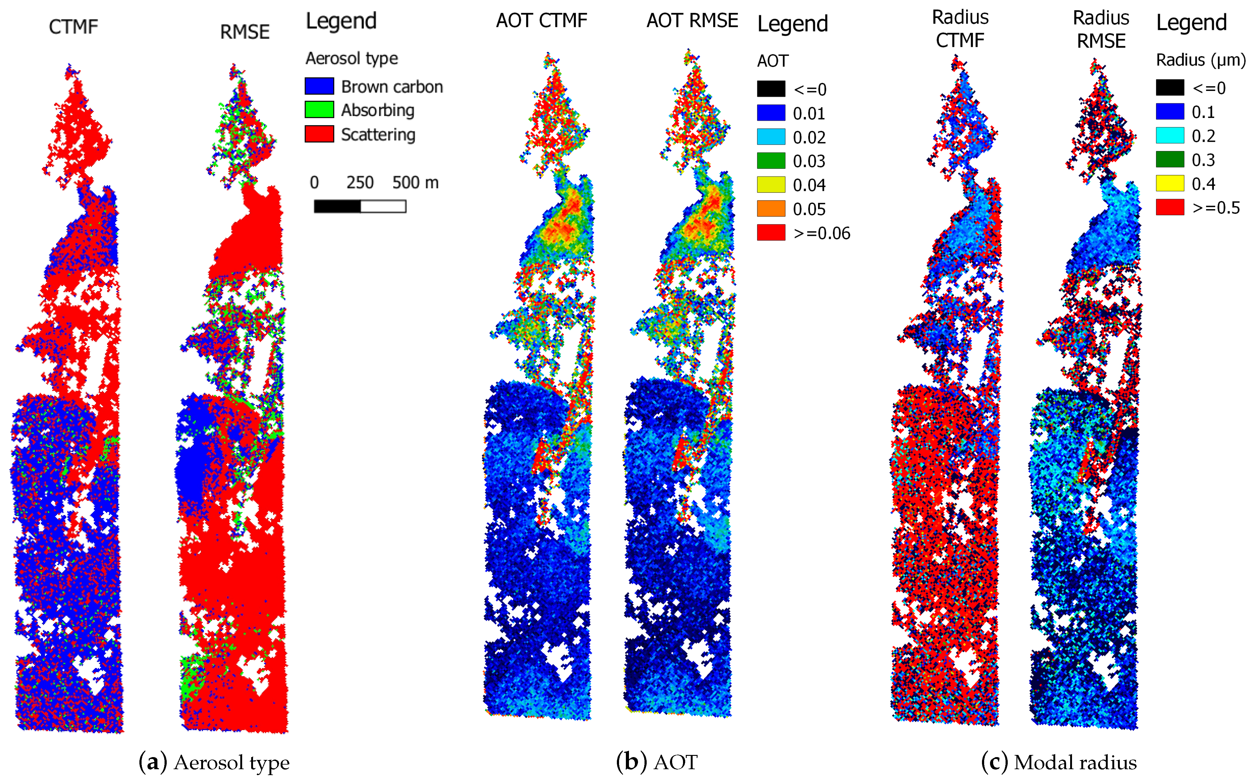
In this stage, we applied the CTMF and RMSE sequential approaches to initialise the plume AOT, modal aerosol radius, and aerosol type pixel-by-pixel. Figure 6 shows maps associated with each metric, and Table 4 corresponds to the mean retrieved values class-by-class. The aerosol type most frequently obtained by the CTMF and the RMSE was a “scattering aerosol”, as is expected from a sinter plant emitter [65,66]. Over the whole image, 70% of the pixels were classified as scattering aerosols for the RMSE method and 45% for the CMTF method. The retrieved modal radii differed between CTMF and RMSE. Over water bodies, the RMSE retrieved modal radii varying from 0.1 to 0.25 m, being close to that found in previous studies over the same area Philippets et al. [10]. However, these values seemed to overestimate in situ measurement over metallurgic plants [65,67]. The CTMF provided higher aerosol radii (higher than 0.5 m) over water bodies, where the AOTs of the plume were below 0.02, but provided similar radii as the RMSE method for larger AOTs in the densest part of the plume. Over artificial soils, the mean retrieved radius was about 0.4 m for the CTMF and 0.25 m for RMSE; additionally, 33% and 38% of the retrieved radii were higher than 0.5 m for the RMSE and CMTF methods, respectively. As mentioned in Section 4.3, the surface reflectance correction was less consistent over artificial and bright soils. For the surface reflectances of the artificial and bright soils, both methods tended to overestimate the radius and AOT, compared to that for water surfaces, where the error of the estimated surface reflectance was low.

Figure 6.
Retrieved plume aerosol parameters: (a) model, (b) AOT, and (c) modal radius, using the CTMF compared with the RMSE.

Table 4.
Mean AOT and radius by class of soil, retrieved with the CTMF and RMSE methods.
The retrieved mean AOTs were about 0.02 for both the CTMF and RMSE. The mean difference between AOTs retrieved was lower than 0.01 for all surface reflectance classes, except for the bright soil class (Table 4). For the bright soil class, the mean difference was 0.23.
Figure 7 represents the difference between spectra acquired inside and outside the plume (point B and point A in Figure 3, respectively). The point B spectrum corresponds to a mean of pixels, having a mean AOT of 0.06. The spectra A and B were localised over the water surface and their differential was compared to the differential simulated using aerosol properties from the CTMF or RMSE methods. Mean radii retrieved using CTMF and RMSE were 0.13 m and 0.16 m, respectively. The normalized RMSE of the differential were 9.2% for the CTMF and 6.5% for the RMSE methods, and the corresponding SAM were 5.1 and 3.6, respectively.
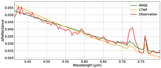
Figure 7.
Example of difference between spectra acquired inside and outside the plume over water surface (red), compared to the best differential model from the CTMF (orange) and RMSE (green) approaches.
In general, the differential calculated with the radius obtained by the RMSE method better corresponded to the observations for all the soil classes, although there were still high radius values for artificial soils. The CTMF formulation is well-adapted for gases with a signature defined by local absorption bands; however, due to the correlations between the spectral signatures of aerosols and their influence on the slope of the entire spectrum, the CTMF results led to a high error rate on the type of aerosol. The RMSE, therefore, seems to best provide a first estimate of the modal radius and the AOT. In addition, the RMSE provides an estimate of the and parameters. Minimization of RMSE in the densest part (i.e., at the center) of the plume corresponded to values of 0 for and 0.3 for .
4.6. Results of the Optimal Estimation Method
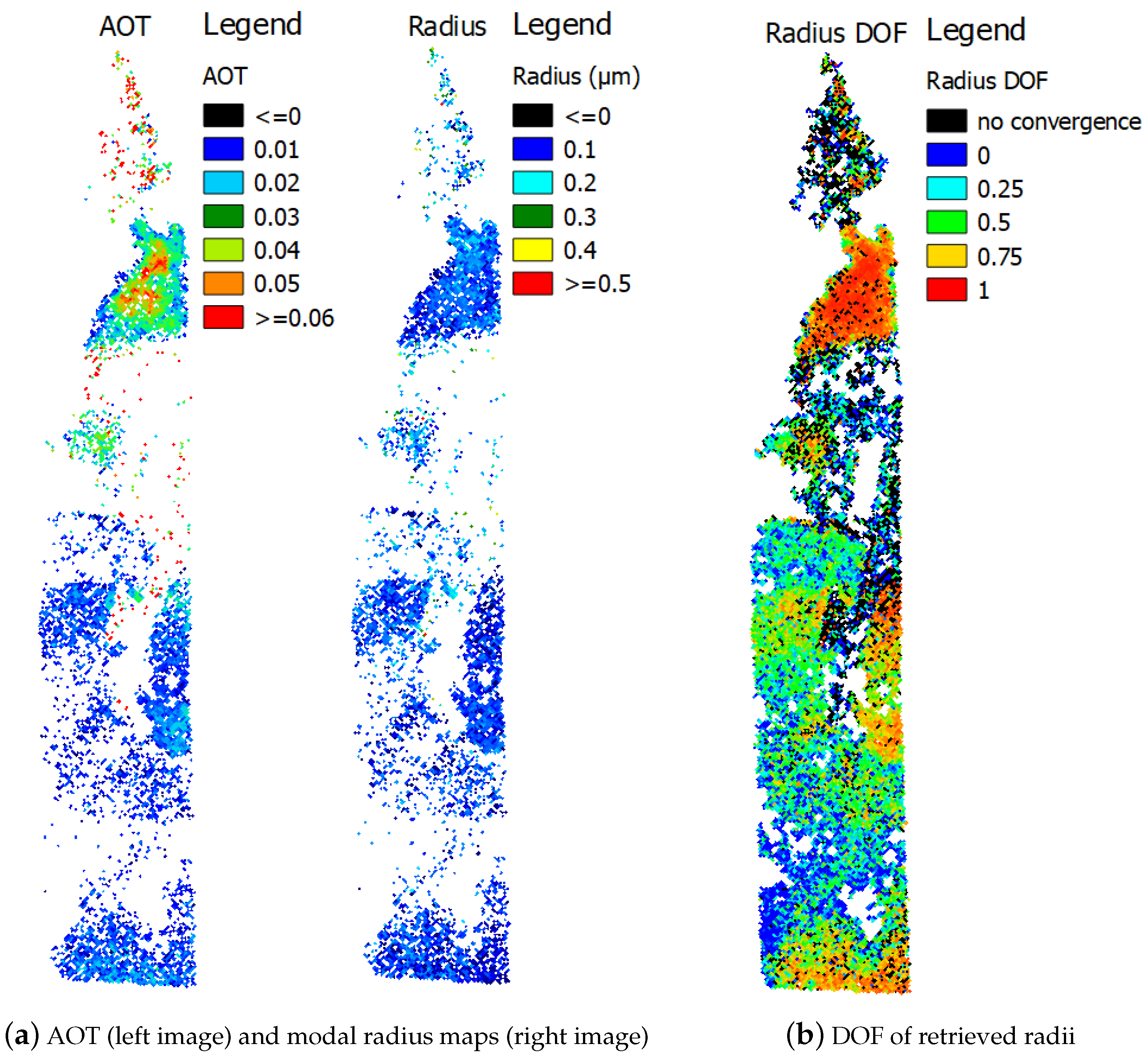
OEM (see framework in Section 2.2) accounted for the errors associated with the prior parameters, the observations, and the atmospheric correction. The OEM was initialized with the AOT and modal radius retrieved from RMSE sequential approach and with the surface reflectances under the plume estimated by the CNMF. AOT, modal radius, and surface reflectance maps, with their associated posteriori uncertainties and their DOF, were then retrieved. Figure 8a illustrates these results. Low DOF values indicate a retrieval being dependent on a priori information, meaning that, due to the large initial error (reflectance and/or aerosol properties), the residual was too high when compared to a priori uncertainties. Only pixels with a retrieved radius with DOF > 0.5 were used to post-process the retrieved maps of AOT and modal radius (see Figure 8). Pixels for which the OEM failed to converge were included in the rejection mask. This rejection mask was associated with pixels where prior information were not consistent with the measurement and the model. It corresponded, in particular, to pixels over artificial soils near the source point, where the prior radius from RMSE initialization seemed to be overestimated (values larger than 0.5 m). Table 5 shows the mean radius retrieved by the OEM class-by-class. The mean retrieved radius in the entire plume was 0.125 m, with a standard deviation of 0.05 m. In comparison, inside the final plume mask, the initial mean radius was around 0.15 m, with a standard deviation of 0.1 m. This decrease in the mean radius led to a slight decrease in the AOT—in particular, for bright surfaces. Near the source, the mean retrieved radii were between 0.1 and 0.2 m and the AOT was above 0.05. Downwind of the source point over water bodies, the mean retrieved radius was 0.12 m, with a standard deviation of about 0.04 m, while the retrieved AOT varied from 0.01 to 0.07. Over sparse vegetation soils, the DOF were lower than over water bodies, with values varying from 0.2 to 0.7; furthermore, the mean retrieved radius was around 0.15 m, with a standard deviation of about 0.07 m. Table 5 shows that the variation of the mean modal radius from one class to another was reduced from the initial guess. OEM-retrieved values were more homogeneous spatially than in the a priori. These results show that, over the whole plume, the size distribution was fairly stable—corresponding to an ultra-fine mode.
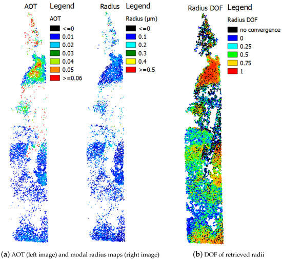
Figure 8.
OEM-retrieved: (a) AOT and modal radius; and (b) radius DOF map.

Table 5.
Mean radius (m) by class of soil, retrieved with the OEM methods and from the initial guess inside the final plume mask.
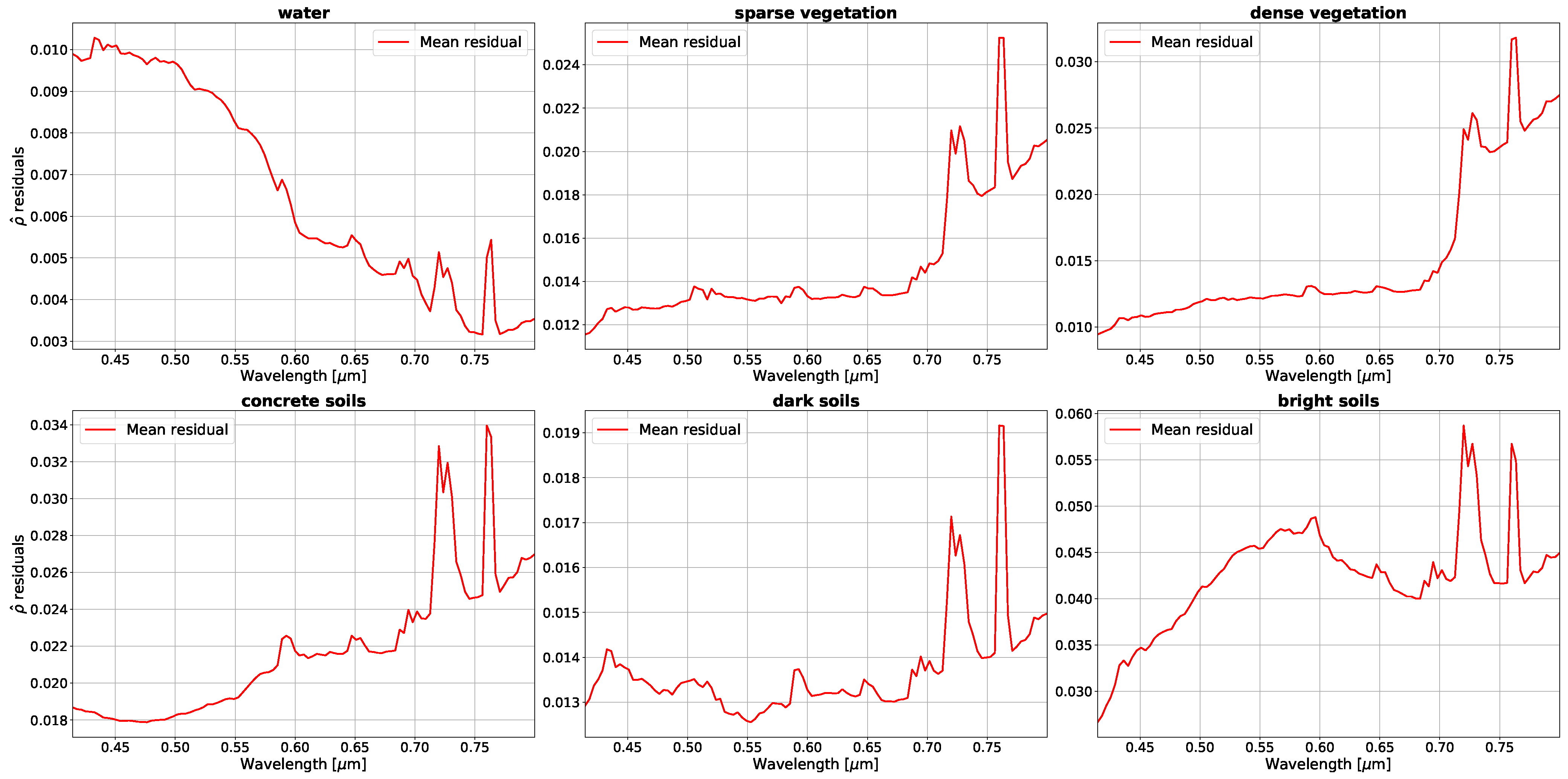
The residual errors associated with the retrieval for different surface categories are presented in Table 6. Figure 9 illustrates the mean standard deviations by class of soil of posterior uncertainties on the retrieved surface reflectances.

Table 6.
Mean standard deviations of the posterior uncertainties in AOT and modal radius by surface categories. The uncertainty from the measurement and from the resolving error component are associated with this standard deviation.
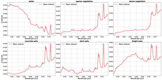
Figure 9.
Mean standard deviation of posteriori uncertainties on surface reflectance as a function of wavelength and by surface category.
The main part of the error came from the resolving error (see Table 6), except for the water surface, where the error was driven by the measurement noise. Radius uncertainties from Table 6 were not really dependent on the class, with a mean value around 0.05; this value was coherent with the standard deviation estimated from the OEM radius map. However, radius prior uncertainties remained larger for bright surfaces and vegetation surfaces.
AOT posterior uncertainties depended on the type of surface, with values varying from 0.003 for water to 0.013 for bright soils. This means that the OEM surface reflectance retrieval did not compensate completely for the initial error in the surface reflectance estimation computed with the CNMF. As shown in Figure 9, the reflectance posterior uncertainty for bright surfaces, vegetation, and concrete soil were higher than for water reflectance spectra. For water surfaces, the mean posterior reflectance uncertainties were less than 0.01, which led to less uncertainty in the retrieved AOT. For bright surfaces, the mean reflectance uncertainties increased up to 0.045, leading to larger uncertainties (Table 6).
Finally, the OEM-retrieved plume parameters were less sensitive to ground heterogeneity than the initial sequential approach. The estimated mean modal radius was about 0.125 m, with a standard deviation of about 0.05 m. Moreover, the OEM helped to enhance the quality of the retrieval, by rejecting pixels where the prior information was not consistent with model uncertainties.
5. Discussion
5.1. Retrieved Modal Radius
The size distribution retrieved in the plume corresponded to an ultra-fine log-normal mode, having a modal radius of 0.125 m and a standard deviation of 1.5. The retrieved size distribution was in agreement with previous work based on airborne hyperspectral data on the same plant, which gave a modal radius around 0.2 m [10,66]. In situ observations over two metallurgic sites in Europe [65,67] have shown that the particle size distribution inside the plume and near the source corresponds to an ultra-fine mode with a modal radius that is (most of the time) less than 0.1 m, with a standard deviation around 1.5. Aerosols in the ultra-fine fraction are formed by secondary aerosols in the Aitken mode, which coagulate downwind the plume [65] and contain metal-bearing nanoparticles [67]. The contribution of fine particles (PM) can be up to 60% for metallurgy, although the PM fraction depends on the industrial process [68]. A similar result has been obtained for a refinery plume using hyperspectral airborne imagery [11], which showed a retrieved particle size distribution corresponding to the ultra-fine mode (modal radius around 100 nm). An absorbing fraction of around 10% has been found in the refinery plume, while only a scattering aerosol was retrieved in the metallurgy plume.
Although the hyperspectral retrievals indicate the presence of ultra-fine particles, it is expected to have a contribution of larger particles (PM) inside the plume [68]. However, the sensitivity of VNIR radiances to the aerosol coarse mode with a modal radius higher than 1 m is weak. Increasing the standard deviation of the size distribution (e.g., from 1.5 to 2.0) lowered the retrieved radius (by 0.05 m, respectively) in areas with DOF > 0.5, indicating a competitive impact of the modal radius and the standard deviation on the retrieval. This confirms that, in the VNIR spectral domain, the observed plume signature has a very weak contribution of coarse aerosols. The addition of a coarse mode in the aerosol forward model, as associated with an extension of the retrieval spectral range to the SWIR domain, may help to infer the contribution of the different aerosol modes.
5.2. Ground Reflectance Estimation and OEM
The surface reflectance estimation accuracy in the initialization step has a major impact on the retrieval uncertainties. Particularly in the case of bright surfaces, any bias or offset on the estimated reflectances must be avoided. Using a single hyperspectral image to estimate the ground reflectance can lead to large errors, as was seen in Section 4.2 and Section 4.3. The use of MSI data in the classification allows for a removal of the radiative impact of the plume (see Figure 4) from the background image and reduction of the intra-class surface reflectance variability, compared to a single hyperspectral acquisition (see Table 3). Moreover, adding the ground reflectance as a retrieved parameter in the OEM process decreases the reflectance uncertainties, compared to the initial stage. Consequently, the reflectance uncertainty can be reduced by a factor of 2 (see Figure 9) for bright and concrete soils. Considering a further application to hyperspectral space missions, such as PRISMA [69], the reflectance error estimation could be reduced, as: (i) the spatial heterogeneity will decrease, due to the lower spatial resolution (30 m instead 10 m); (ii) the signal-to-noise ratio is similar to HYSPEX noise (see Figure 2b); and (iii) the fusion algorithms will not have to deal with a change of spectral resolution. Additionally, we notice that the OEM also helps to reject the pixels which have an estimated ground reflectance error too high and/or with a false positive plume detection, thanks to the DOF and the algorithm convergence.
5.3. Model Assumptions and Uncertainties
From sensitivity and posteriori uncertainty analyses, we saw that the modal radius uncertainty of 0.05 m was quite independent of the reflectance value, whereas the AOT error increased with the reflectance value (from 0.003 to 0.01). Moreover, the non-retrieved b state vector used in the results section did not include all the forward model assumption uncertainties or errors described in the method section. In particular, the aerosol plume refractive index uncertainty and size distribution standard deviation are important sources of error for the AOT (0.008) and modal radius (0.045 m), respectively. This means that the a posteriori uncertainties estimated in the results section were underestimated, particularly for low reflectance values. We assumed that the real uncertainties were around 0.01 for AOT and around 0.06 m for the modal radius. Some forward model assumptions are still missing in the total budget error, such as the environmental effects and the uncertainty in the imaginary part of the refractive index.
6. Conclusions
Stack plume detection and characterization over a metallurgic plant were performed with the use of airborne hyperspectral data. The proposed method relies on the combination of hyperspectral acquisition with additional Sentinel-2/MSI surface reflectances. The spatial resolution of the product was 10 m, matching the satellite data. The MSI data provided an off-plume background image of the scene and, so, reduced the error in both plume segmentation and the estimation of aerosol optical properties.
A first guess of the plume aerosol optical properties, in terms of modal radius and AOT, was performed using a sequential method. The previously proposed CTMF method was outperformed by the RMSE metric in the sequential approach. The OEM improved the consistency of the retrieval and provided an estimation of the error balance, by simultaneously retrieving the plume properties and the surface reflectances under the plume. OEM provides the opportunity to analyse uncertainties through an analytical equation system. It can provide information (gain matrix) and criteria (degree of freedom) on the retrieval sensitivity of plume properties above several ground types, with respect to the observation noise. The observed plume was optically thin, with AOT lower than 0.1 and a detection threshold around 0.01. The retrieved size distribution mode corresponded to a fine (i.e., ultra-fine) mode with a modal radius of 0.125 m and a log-normal distribution standard deviation of 1.5. All of the detected pixels had a DOF higher than 0.5 and the average a posteriori uncertainties of the estimates were 0.01 for the AOT and 0.06 m for the modal radius. These results were close to the ultra-fine mode (modal radius around 0.1 m) observed from in situ measurements within the plumes of metallurgical plants [65,67].
Knowledge of PM atmospheric concentrations from industrial stack plumes and associated emission fluxes from satellite observations could allow for a better assessment of the impact of industrial emissions on air quality at a high spatial resolution. The proposed method to retrieve aerosol optical properties and evaluate the associated uncertainties serves as a first step toward this objective. We also showed the potential and feasibility of combining hyperspectral data with other satellite data with different spectral and spatial resolutions, but higher temporal frequency. The proposed framework can be applied to current hyperspectral satellite missions, in combination with the available Sentinel-2 products.
Author Contributions
Conceptualization, P.-Y.F. and J.-F.L.; methodology, P.-Y.F., J.-F.L., and G.C.; software, G.C.; investigation, G.C.; writing—original draft preparation, G.C.; writing—review and editing, J.-F.L.; supervision, P.-Y.F. and J.-F.L. All authors have read and agreed to the published version of the manuscript.
Funding
This work was supported by CNES under contract named IMHYS-Apport de de l’imagerie hyperspectrale satellite pour le suivi des sources d’aérosols anthropiques. Gabriel Calassou’s thesis is co-funded by ONERA, The French Aerospace Lab and CNES.
Institutional Review Board Statement
Not applicable.
Informed Consent Statement
Not applicable.
Data Availability Statement
The data presented in this study are available on request from the corresponding author. The data are not publicly available due to the ONERA internal policy.
Acknowledgments
The authors would like to thank Yokoya for sharing their code on CNMF. Sentinel-2/MSI data used in this paper are Copernicus data process by CNES for the THEIA thematic center.
Conflicts of Interest
The authors declare no conflict of interest.
References
- World Health Organization. Health Risks of Particulate Matter from Long-Range Transboundary Air Pollution; World Health Organization: Geneva, Switzerland, 2006. [Google Scholar]
- Burnett, R.; Chen, H.; Szyszkowicz, M.; Fann, N.; Hubbell, B.; Pope, C.A.; Apte, J.S.; Brauer, M.; Cohen, A.; Weichenthal, S.; et al. Global Estimates of Mortality Associated with Long-term Exposure to Outdoor Fine Particulate Matter. Proc. Natl. Acad. Sci. USA 2018, 115, 9592–9597. [Google Scholar] [CrossRef]
- National Emissions Reported to the Convention on Long-Range Transboundary Air Pollution (LRTAP Convention)—European Environment Agency. Available online: https://www.eea.europa.eu/data-and-maps/data/national-emissions-reported-to-the-convention-on-long-range-transboundary-air-pollution-lrtap-convention-14 (accessed on 14 December 2020).
- European Environment Agency. EMEP/EEA Air Pollutant Emission Inventory Guidebook 2019: Technical Guidance to Prepare National Emission Inventories; European Environment Agency: Copenhagen, Denmark, 2019.
- Andre, J.M.; Barrault, S.; Bongrand, G.; Bort, R.; Cuniasse, B.; Druart, A.; Durand, A.; Feutren, E.; Gavel, A.; Glass, T.; et al. Rapport Ominea, 16th ed.; Technical Report; 2019. Available online: https://www.citepa.org/fr/ominea/ (accessed on 8 May 2021).
- Amaral, S.; de Carvalho, J.; Costa, M.; Pinheiro, C. An Overview of Particulate Matter Measurement Instruments. Atmosphere 2015, 6, 1327–1345. [Google Scholar] [CrossRef]
- Stull, R.B. An Introduction to Boundary Layer Meteorology; Atmospheric and Oceanographic Sciences Library; Springer: Dordrecht, The Netherlands, 1988. [Google Scholar] [CrossRef]
- Gordon, M.; Makar, P.A.; Staebler, R.M.; Zhang, J.; Akingunola, A.; Gong, W.; Li, S.M. A Comparison of Plume Rise Algorithms to Stack Plume Measurements in the Athabasca Oil Sands. Atmos. Chem. Phys. 2018, 18, 14695–14714. [Google Scholar] [CrossRef]
- Alakian, A.; Marion, R.; Briottet, X. Retrieval of Microphysical and Optical Properties in Aerosol Plumes with Hyperspectral Imagery: L-APOM Method. Remote Sens. Environ. 2009, 113, 781–793. [Google Scholar] [CrossRef]
- Philippets, Y.; Foucher, P.Y.; Marion, R.; Briottet, X. Anthropogenic Aerosol Emissions Mapping and Characterization by Imaging Spectroscopy–Application to a Metallurgical Industry and a Petrochemical Complex. Int. J. Remote Sens. 2018, 40, 364–406. [Google Scholar] [CrossRef]
- Foucher, P.Y.; Deliot, P.; Poutier, L.; Duclaux, O.; Raffort, V.; Roustan, Y.; Temime-Roussel, B.; Durand, A.; Wortham, H. Aerosol Plume Characterization from Multitemporal Hyperspectral Analysis. IEEE J. Sel. Top. Appl. Earth Obs. Remote Sens. 2019, 12, 2429–2438. [Google Scholar] [CrossRef]
- Kaufman, Y.J.; Sendra, C. Algorithm for Automatic Atmospheric Corrections to Visible and Near-IR Satellite Imagery. Int. J. Remote Sens. 1988, 9, 1357–1381. [Google Scholar] [CrossRef]
- Kaufman, Y.J.; Tanré, D.; Gordon, H.R.; Nakajima, T.; Lenoble, J.; Frouin, R.; Grassl, H.; Herman, B.M.; King, M.D.; Teillet, P.M. Passive Remote Sensing of Tropospheric Aerosol and Atmospheric Correction for the Aerosol Effect. J. Geophys. Res. Atmos. 1997, 102, 16815–16830. [Google Scholar] [CrossRef]
- Levy, R.C.; Remer, L.A.; Kleidman, R.G.; Mattoo, S.; Ichoku, C.; Kahn, R.; Eck, T.F. Global Evaluation of the Collection 5 MODIS Dark-target Aerosol Products Over Land. Atmos. Chem. Phys. 2010, 10, 10399–10420. [Google Scholar] [CrossRef]
- Remer, L.A.; Levy, R.C.; Mattoo, S.; Tanré, D.; Gupta, P.; Shi, Y.; Sawyer, V.; Munchak, L.A.; Zhou, Y.; Kim, M.; et al. The Dark Target Algorithm for Observing the Global Aerosol System: Past, Present, and Future. Remote Sens. 2020, 12, 2900. [Google Scholar] [CrossRef]
- Hsu, N.; Tsay, S.C.; King, M.; Herman, J. Aerosol Properties Over Bright-Reflecting Source Regions. IEEE Trans. Geosci. Remote Sens. 2004, 42, 557–569. [Google Scholar] [CrossRef]
- Hsu, N.; Tsay, S.C.; King, M.; Herman, J. Deep Blue Retrievals of Asian Aerosol Properties during ACE-asia. IEEE Trans. Geosci. Remote Sens. 2006, 44, 3180–3195. [Google Scholar] [CrossRef]
- Sayer, A.M.; Hsu, N.C.; Lee, J.; Kim, W.V.; Dutcher, S.T. Validation, Stability, and Consistency of MODIS Collection 6.1 and VIIRS Version 1 Deep Blue Aerosol Data Over Land. J. Geophys. Res. Atmos. 2019, 124, 4658–4688. [Google Scholar] [CrossRef]
- Thomas, G.E.; Poulsen, C.A.; Sayer, A.M.; Marsh, S.H.; Dean, S.M.; Carboni, E.; Siddans, R.; Grainger, R.G.; Lawrence, B.N. The GRAPE Aerosol Retrieval Algorithm. Atmos. Meas. Tech. 2009, 2, 679–701. [Google Scholar] [CrossRef]
- Dubovik, O.; Herman, M.; Holdak, A.; Lapyonok, T.; Tanré, D.; Deuzé, J.L.; Ducos, F.; Sinyuk, A.; Lopatin, A. Statistically Optimized Inversion Algorithm for Enhanced Retrieval of Aerosol Properties from Spectral Multi-Angle Polarimetric Satellite Observations. Atmos. Meas. Tech. 2011, 4, 975–1018. [Google Scholar] [CrossRef]
- Wurl, D.; Grainger, R.G.; McDonald, A.J.; Deshler, T. Optimal Estimation Retrieval of Aerosol Microphysical Properties from SAGE~II Satellite Observations in the Volcanically Unperturbed Lower Stratosphere. Atmos. Chem. Phys. 2010, 10, 4295–4317. [Google Scholar] [CrossRef]
- Zheng, F.; Hou, W.; Sun, X.; Li, Z.; Hong, J.; Ma, Y.; Li, L.; Li, K.; Fan, Y.; Qiao, Y. Optimal Estimation Retrieval of Aerosol Fine-Mode Fraction from Ground-Based Sky Light Measurements. Atmosphere 2019, 10, 196. [Google Scholar] [CrossRef]
- Govaerts, Y.M.; Wagner, S.; Lattanzio, A.; Watts, P. Joint retrieval of surface reflectance and aerosol optical depth from MSG/SEVIRI observations with an optimal estimation approach: 1. Theory. J. Geophys. Res. 2010, 115. [Google Scholar] [CrossRef]
- Thompson, D.R.; Natraj, V.; Green, R.O.; Helmlinger, M.C.; Gao, B.C.; Eastwood, M.L. Optimal Estimation for Imaging Spectrometer Atmospheric Correction. Remote Sens. Environ. 2018, 216, 355–373. [Google Scholar] [CrossRef]
- Thompson, D.R.; Babu, K.; Braverman, A.J.; Eastwood, M.L.; Green, R.O.; Hobbs, J.M.; Jewell, J.B.; Kindel, B.; Massie, S.; Mishra, M.; et al. Optimal Estimation of Spectral Surface Reflectance in Challenging Atmospheres. Remote Sens. Environ. 2019, 232, 111258. [Google Scholar] [CrossRef]
- Hou, W.; Wang, J.; Xu, X.; Reid, J.S.; Han, D. An Algorithm for Hyperspectral Remote Sensing of Aerosols: 1. Development of Theoretical Framework. J. Quant. Spectrosc. Radiat. Transf. 2016, 178, 400–415. [Google Scholar] [CrossRef]
- Hou, W.; Wang, J.; Xu, X.; Reid, J.S. An Algorithm for Hyperspectral Remote Sensing of Aerosols: 2. Information Content Analysis for Aerosol Parameters and Principal Components of Surface Spectra. J. Quant. Spectrosc. Radiat. Transf. 2017, 192, 14–29. [Google Scholar] [CrossRef]
- Rodgers, C.D. Inverse Methods for Atmospheric Sounding; World Scientific: Singapore, 2000. [Google Scholar] [CrossRef]
- Kangah, K.G.Y. Measurement of Nitrous Oxide (N2O) from Space. Ph.D. Thesis, Université Paul Sabatier-Toulouse III, Toulouse, France, 2017. [Google Scholar]
- Hurtmans, D.; Coheur, P.F.; Wespes, C.; Clarisse, L.; Scharf, O.; Clerbaux, C.; Hadji-Lazaro, J.; George, M.; Turquety, S. FORLI Radiative Transfer and Retrieval Code for IASI. J. Quant. Spectrosc. Radiat. Transf. 2012, 113, 1391–1408. [Google Scholar] [CrossRef]
- Barret, B.; Flochmoen, E.L.; Sauvage, B.; Pavelin, E.; Matricardi, M.; Cammas, J.P. The Detection of Post-monsoon Tropospheric Ozone Variability Over South Asia Using IASI Data. Atmos. Chem. Phys. 2011, 11, 9533–9548. [Google Scholar] [CrossRef]
- Yoshida, Y.; Ota, Y.; Eguchi, N.; Kikuchi, N.; Nobuta, K.; Tran, H.; Morino, I.; Yokota, T. Retrieval Algorithm for CO2 and CH4 Column Abundances from Short-wavelength Infrared Spectral Observations by the Greenhouse Gases Observing Satellite. Atmos. Meas. Tech. 2011, 4, 717–734. [Google Scholar] [CrossRef]
- Hagolle, O.; Huc, M.; Desjardins, C.; Auer, S.; Richter, R. Maja Algorithm Theoretical Basis Document. 2017. Available online: https://doi.org/10.5281/ZENODO.1209633 (accessed on 8 May 2021).
- Dubovik, O.; Lapyonok, T.; Litvinov, P.; Herman, M.; Fuertes, D.; Ducos, F.; Torres, B.; Derimian, Y.; Huang, X.; Lopatin, A.; et al. GRASP: A Versatile Algorithm for Characterizing the Atmosphere. SPIE Newsroom 2014. [Google Scholar] [CrossRef]
- Qu, Z.; Kindel, B.; Goetz, A. The High Accuracy Atmospheric Correction for Hyperspectral Data (hatch) Model. IEEE Trans. Geosci. Remote Sens. 2003, 41, 1223–1231. [Google Scholar] [CrossRef]
- Adler-Golden, S.M.; Matthew, M.W.; Bernstein, L.S.; Levine, R.Y.; Berk, A.; Richtsmeier, S.C.; Acharya, P.K.; Anderson, G.P.; Felde, J.W.; Gardner, J.A.; et al. Atmospheric Correction for Shortwave Spectral Imagery Based on MODTRAN4; Descour, M.R., Shen, S.S., Eds.; Imaging Spectrometry V; SPIE: Bellingham, WA, USA, 1999. [Google Scholar] [CrossRef]
- Staenz, K.; Szeredi, T.; Schwarz, J. ISDAS—A System for Processing/analyzing Hyperspectral Data. Can. J. Remote Sens. 1998, 24, 99–113. [Google Scholar] [CrossRef]
- Richter, R. Atmospheric Correction of DAIS Hyperspectral Image Data. Comput. Geosci. 1996, 22, 785–793. [Google Scholar] [CrossRef]
- Richter, R. Correction of Satellite Imagery Over Mountainous Terrain. Appl. Opt. 1998, 37, 4004. [Google Scholar] [CrossRef]
- Richter, R.; Schläpfer, D. Geo-atmospheric Processing of Airborne Imaging Spectrometry Data. Part 2: Atmospheric/topographic Correction. Int. J. Remote Sens. 2002, 23, 2631–2649. [Google Scholar] [CrossRef]
- Chandrasekhar, S. Radiative Transfer; Dover Publications: New York, NY, USA, 1960. [Google Scholar]
- Alakian, A.; Marion, R.; Briottet, X. Remote Sensing of Aerosol Plumes: A Semianalytical Model. Appl. Opt. 2008, 47, 1851. [Google Scholar] [CrossRef]
- Poutier, L.; Miesch, C.; Lenot, X.; Achard, V.; Boucher, Y. COMANCHE and COCHISE: Two reciprocal atmospheric codes for hyperspectral remote sensing. In Proceedings of the 2002 AVIRIS Earth Science and Applications Workshop Proceedings, Pasadena, CA, USA, 5–8 March 2002. [Google Scholar]
- Berk, A.; Conforti, P.; Kennett, R.; Perkins, T.; Hawes, F.; van den Bosch, J. MODTRAN® 6: A Major Upgrade of the MODTRAN® Radiative Transfer Code. In Proceedings of the 2014 6th Workshop on Hyperspectral Image and Signal Processing: Evolution in Remote Sensing (WHISPERS), Lausanne, Switzerland, 24–27 June 2014. [Google Scholar] [CrossRef]
- Ångström, A. On the Atmospheric Transmission of Sun Radiation and on Dust in the Air. Geogr. Ann. 1929, 11, 156–166. [Google Scholar] [CrossRef]
- QGIS Development Team. QGIS Geographic Information System. Open Source Geospatial Foundation. 2020. Available online: http://qgis.osgeo.org (accessed on 12 March 2021).
- Eismann, M.T.; Hardie, R.C. Resolution enhancement of hyperspectral imagery using coincident panchromatic imagery and a stochastic mixing model. In Proceedings of the IEEE Workshop on Advances in Techniques for Analysis of Remotely Sensed Data, Greenbelt, MD, USA, 27–28 October 2003; pp. 282–289. [Google Scholar] [CrossRef]
- Lanaras, C.; Baltsavias, E.; Schindler, K. Hyperspectral Super-resolution by Coupled Spectral Unmixing. In Proceedings of the 2015 IEEE International Conference on Computer Vision (ICCV), Santiago, Chile, 7–13 December 2015. [Google Scholar] [CrossRef]
- Simoes, M.; Bioucas-Dias, J.; Almeida, L.B.; Chanussot, J. A Convex Formulation for Hyperspectral Image Superresolution Via Subspace-based Regularization. IEEE Trans. Geosci. Remote Sens. 2015, 53, 3373–3388. [Google Scholar] [CrossRef]
- Wei, Q.; Dobigeon, N.; Tourneret, J.Y. Fast Fusion of Multi-band Images Based on Solving a Sylvester Equation. IEEE Trans. Image Process. 2015, 24, 4109–4121. [Google Scholar] [CrossRef]
- Yokoya, N.; Yairi, T.; Iwasaki, A. Coupled Nonnegative Matrix Factorization Unmixing for Hyperspectral and Multispectral Data Fusion. IEEE Trans. Geosci. Remote Sens. 2012, 50, 528–537. [Google Scholar] [CrossRef]
- Nascimento, J.; Dias, J. Vertex Component Analysis: A Fast Algorithm to Unmix Hyperspectral Data. IEEE Trans. Geosci. Remote Sens. 2005, 43, 898–910. [Google Scholar] [CrossRef]
- Liu, X.; Xia, W.; Wang, B.; Zhang, L. An Approach Based on Constrained Nonnegative Matrix Factorization to Unmix Hyperspectral Data. IEEE Trans. Geosci. Remote Sens. 2011, 49, 757–772. [Google Scholar] [CrossRef]
- Lee, D.D.; Seung, H.S. Learning the Parts of Objects by Non-negative Matrix Factorization. Nature 1999, 401, 788–791. [Google Scholar] [CrossRef]
- Funk, C.C.; Theiler, J.; Roberts, D.A.; Borel, C.C. Clustering to Improve Matched Filter Detection of Weak Gas Plumes in Hyperspectral Thermal Imagery. IEEE Trans. Geosci. Remote Sens. 2001, 39, 1410–1420. [Google Scholar] [CrossRef]
- Thorpe, A.K.; Roberts, D.A.; Dennison, P.E.; Bradley, E.S.; Funk, C.C. Point Source Emissions Mapping Using the Airborne Visible/infrared Imaging Spectrometer (AVIRIS). In Algorithms and Technologies for Multispectral, Hyperspectral, and Ultraspectral Imagery XVIII; Shen, S.S., Lewis, P.E., Eds.; SPIE: Bellingham, WA, USA, 2012. [Google Scholar] [CrossRef]
- Thorpe, A.; Frankenberg, C.; Aubrey, A.; Roberts, D.; Nottrott, A.; Rahn, T.; Sauer, J.; Dubey, M.; Costigan, K.; Arata, C.; et al. Mapping Methane Concentrations from a Controlled Release Experiment Using the Next Generation Airborne Visible/infrared Imaging Spectrometer (AVIRIS-NG). Remote Sens. Environ. 2016, 179, 104–115. [Google Scholar] [CrossRef]
- Dennison, P.E.; Thorpe, A.K.; Pardyjak, E.R.; Roberts, D.A.; Qi, Y.; Green, R.O.; Bradley, E.S.; Funk, C.C. High Spatial Resolution Mapping of Elevated Atmospheric Carbon Dioxide Using Airborne Imaging Spectroscopy: Radiative Transfer Modeling and Power Plant Plume Detection. Remote Sens. Environ. 2013, 139, 116–129. [Google Scholar] [CrossRef]
- Institut Géographique National. Géoservices|Pourquoi #ChoisirGéoportail? Available online: https://geoservices.ign.fr/documentation/ (accessed on 16 December 2020).
- Brigot, G.; Colin-Koeniguer, E.; Plyer, A.; Janez, F. Adaptation and Evaluation of an Optical Flow Method Applied to Coregistration of Forest Remote Sensing Images. IEEE J. Sel. Top. Appl. Earth Obs. Remote Sens. 2016, 9, 2923–2939. [Google Scholar] [CrossRef]
- Plyer, A.; Colin-Koeniguer, E.; Weissgerber, F. A New Coregistration Algorithm for Recent Applications on Urban SAR Images. IEEE Geosci. Remote Sens. Lett. 2015, 12, 2198–2202. [Google Scholar] [CrossRef]
- Hagolle, O.; Huc, M.; Pascual, D.V.; Dedieu, G. A Multi-temporal and Multi-spectral Method to Estimate Aerosol Optical Thickness Over Land, for the Atmospheric Correction of FormoSat-2, LandSat, VENμs and Sentinel-2 Images. Remote Sens. 2015, 7, 2668–2691. [Google Scholar] [CrossRef]
- THEIA-LAND. Available online: https://www.theia-land.fr/pole-theia-2/infrastructure-de-donnees-et-de-services-ids/muscate-2/ (accessed on 16 March 2021).
- Kruse, F.; Lefkoff, A.; Boardman, J.; Heidebrecht, K.; Shapiro, A.; Barloon, P.; Goetz, A. The spectral image processing system (SIPS)—interactive visualization and analysis of imaging spectrometer data. Remote Sens. Environ. 1993, 44, 145–163. [Google Scholar] [CrossRef]
- Leoni, C.; Hovorka, J.; Dočekalová, V.; Cajthaml, T.; Marvanová, S. Source Impact Determination Using Airborne and Ground Measurements of Industrial Plumes. Environ. Sci. Technol. 2016, 50, 9881–9888. [Google Scholar] [CrossRef]
- Deschamps, A. Industrial Plume Characterization Using Hyperspectral Imagery. Ph.D. Thesis, Université Pierre et Marie Curie-Paris VI, Paris, France, 2012. [Google Scholar]
- Marris, H.; Deboudt, K.; Augustin, P.; Flament, P.; Blond, F.; Fiani, E.; Fourmentin, M.; Delbarre, H. Fast changes in chemical composition and size distribution of fine particles during the near-field transport of industrial plumes. Sci. Total Environ. 2012, 427–428, 126–138. [Google Scholar] [CrossRef]
- Ehrlich, C.; Noll, G.; Kalkoff, W.; Baumbach, G.; Dreiseidler, A. PM10, PM2.5 and PM1.0—Emissions from industrial plants—Results from measurement programmes in Germany. Atmos. Environ. 2007, 41, 6236–6254. [Google Scholar] [CrossRef]
- Pignatti, S.; Palombo, A.; Pascucci, S.; Romano, F.; Santini, F.; Simoniello, T.; Umberto, A.; Vincenzo, C.; Acito, N.; Diani, M.; et al. The PRISMA hyperspectral mission: Science activities and opportunities for agriculture and land monitoring. In Proceedings of the 2013 IEEE International Geoscience and Remote Sensing Symposium-IGARSS, Melbourne, Australia, 21–26 July 2013; pp. 4558–4561. [Google Scholar] [CrossRef]
Publisher’s Note: MDPI stays neutral with regard to jurisdictional claims in published maps and institutional affiliations. |
© 2021 by the authors. Licensee MDPI, Basel, Switzerland. This article is an open access article distributed under the terms and conditions of the Creative Commons Attribution (CC BY) license (https://creativecommons.org/licenses/by/4.0/).

