Estimates of Daily Evapotranspiration in the Source Region of the Yellow River Combining Visible/Near-Infrared and Microwave Remote Sensing


Abstract
1. Introduction
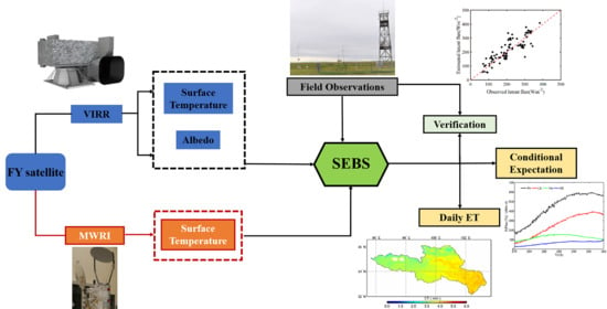
2. Methodology
2.1. Net Radiation
2.1.1. Net Radiation under Clear Sky Conditions
2.1.2. Net Radiation under Cloud Cover
- (1)
- Atmospheric attenuation
- (2)
- The energy received by the satellite sensor
2.2. Soil Heat Flux
2.3. Calculation Method of Sensible Heat Flux
2.4. Evaporation Fraction
2.5. Validation
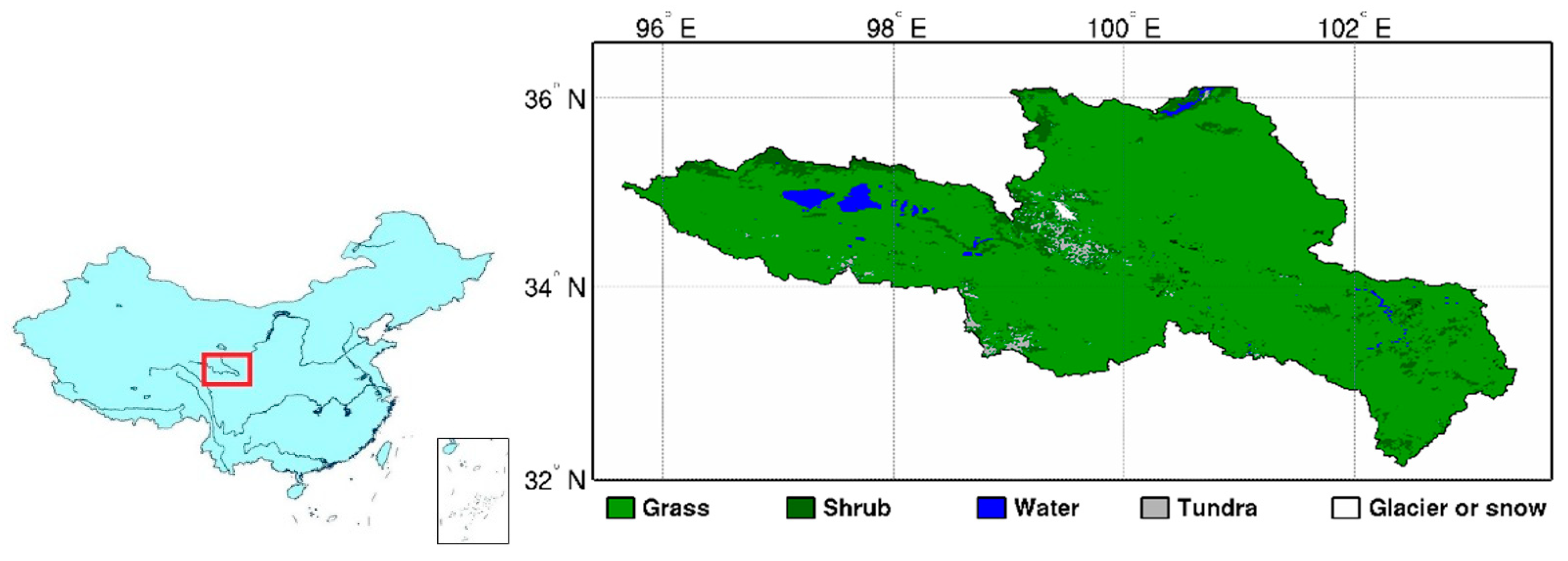
3. Study Area and Observation Data
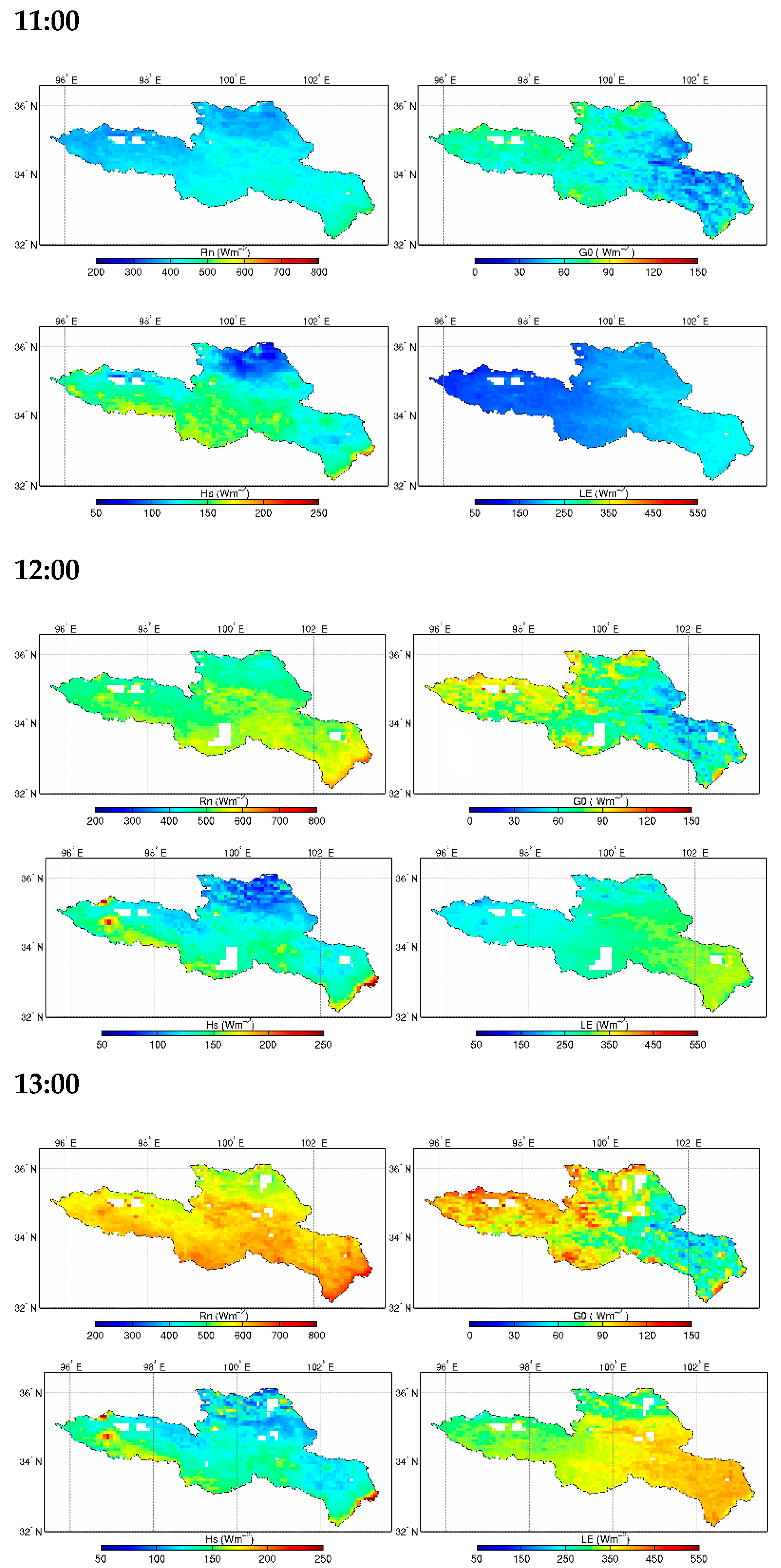
4. Results and Verification
4.1. Results of Energy Flux
4.2. Verification
5. Discussions
5.1. The Relationship between the Conditional Expectation and the Temperature
5.2. The Relationship between Evaporation Fraction, Latent Heat Flux, and Daily ET
5.3. Daily ET
6. Conclusions
Author Contributions
Funding
Institutional Review Board Statement
Informed Consent Statement
Data Availability Statement
Acknowledgments
Conflicts of Interest
References
- Priestley, C.H.B.; Taylor, R.J. On the assessment of surface heat flux and evaporation using large-scale parameters. Mon. Weather Rev. 1972, 100, 81–92. [Google Scholar] [CrossRef]
- Wang, K.C.; Dickinson, R.E. A review of global terrestrial evapotranspiration: Observation, modeling, climatology, and climatic variability. Rev. Geophys. 2012, 50. [Google Scholar] [CrossRef]
- Kim, N.; Kim, K.; Lee, S.; Cho, J.; Lee, Y. Retrieval of daily reference evapotranspiration for croplands in South Korea using machine learning with satellite images and numerical weather prediction data. Remote Sens. 2020, 12, 3642. [Google Scholar] [CrossRef]
- Su, Z.; Schmugge, T.; Kustas, W.P.; Massman, W.J. An evaluation of two models for estimation of the roughness height for heat transfer between the land surface and the atmosphere. J. Appl. Meteorol. 2001, 40, 1933–1951. [Google Scholar] [CrossRef]
- Nedbal, V.; Láska, K.; Brom, J. Mitigation of arctic tundra surface warming by plant evapotranspiration: Complete energy balance component estimation using LANDSAT satellite data. Remote Sens. 2020, 12, 3395. [Google Scholar] [CrossRef]
- Cleugh, H.A.; Lenning, R.; Mu, Q. Regional evaporation estimates from flux tower and MODIS satellite data. Remote Sens. Environ. 2007, 106, 285–304. [Google Scholar] [CrossRef]
- Mu, Q.; Heinsch, F.; Zhao, M.; Running, S. Development of a global evapotranspiration algorithm based on MODIS and global meteorology data. Remote Sens. Environ. 2007, 111, 519–536. [Google Scholar] [CrossRef]
- Jackson, R.D.; Reginato, R.J.; Idso, S.B. Wheat canopy temperature: A practical tool for evaluating water requirements. Water Resour. Res. 1977, 13, 651–656. [Google Scholar] [CrossRef]
- Allen, R.G.; Tasumi, M.; Trezza, R. Satellite-based energy balance for mapping evapotranspiration with internalized calibration (METRIC)-model. J. Irrig. Drain. Eng. 2007, 133, 380–394. [Google Scholar] [CrossRef]
- Carpintero, E.; Mateos, L.; Andreu, A.; González-Dugo, M.P. Effect of the differences in spectral response of Mediterranean tree canopies on the estimation of evapotranspiration using vegetation index-based crop coefficients. Agric. Water Manag. 2020, 238, 106201. [Google Scholar] [CrossRef]
- Jiang, L.; Islam, S. A methodology for estimation of evapotranspiration over large areas using remote sensing information. Geophys. Res. Lett. 1999, 26, 2773–2776. [Google Scholar] [CrossRef]
- Bastiaanssen, W.G.M.; Menenti, M.; Feddes, R.A.; Holtslag, A.A.M. A remote sensing surface energy balance algorithm for land (SEBAL): 1. Formulation. J. Hydrol. 1998, 212–213, 198–212. [Google Scholar] [CrossRef]
- Roerink, G.J.; Su, Z.; Menenti, M. A simple remote sensing algorithm to estimate the surface energy balance. Phys. Chem. Earth 2000, 25, 147–157. [Google Scholar] [CrossRef]
- Su, Z. The surface energy balance system (SEBS) for estimation of turbulent heat fluxes. Hydrol. Earth Syst. Sci. 2002, 6, 85–99. [Google Scholar] [CrossRef]
- Allen, R.G.; Tasumi, M.; Morse, A. Satellite-Based Evapotranspiration by METRIC and Landsat For Western States Water Management; US Bureau of Reclamation Evapotranspiration Workshop: Fort Collins, CO, USA, 2005. [Google Scholar]
- Shuttleworth, W.J.; Wallace, J.S. Evaporation from sparse crops-an energy combination theory. Q. J. R. Meteorol. Soc. 1985, 111, 839–855. [Google Scholar] [CrossRef]
- Norman, J.M.; Kustas, W.P.; Humes, K.S. Source approach for estimating soil and vegetation energy fluxes in observations of directional radiometric surface temperature. Agric. For. Meteorol. 1995, 77, 263–293. [Google Scholar] [CrossRef]
- Chen, S.; Liu, W.H.; Ye, T. Dataset of trend-preserving bias-corrected daily temperature, precipitation and wind from NEX-GDDP and CMIP5 over the Qinghai-Tibet Plateau. Data Brief. 2020, 31, 105733. [Google Scholar] [CrossRef]
- Chen, X.L.; Su, Z.; Ma, Y.M.; Yang, K.; Wang, B. Estimation of surface energy fluxes under complex terrain of Mt. Qomolangma over the Tibetan Plateau. Hydrol. Earth Syst. Sci. 2013, 17, 1607–1618. [Google Scholar] [CrossRef]
- Brutsaert, W. On a derivable formula for long-wave radiation from clear skies. Water Resour. Res. 1975, 11, 742–744. [Google Scholar] [CrossRef]
- Liu, R.; Wen, J.; Wang, X.; Zhang, Y. Evapotranspiration estimated by using datasets from the Chinese FengYun-2D geostationary meteorological satellite over the Yellow River source area. Adv. Space Res. 2015, 55, 60–71. [Google Scholar] [CrossRef]
- Li, X.Q.; Yang, H.; You, R. Remote sensing typhoon Songda’s rainfall structure based on Microwave Radiation Imager of FY-3B satellite. Chin. J. Geophys. 2013, 28, 875–889. (In Chinese) [Google Scholar]
- Han, C.; Ma, Y.; Chen, X.; Su, Z. Trends of land surface heat fluxes on the Tibetan Plateau from 2001 to 2012. Int. J. Clim. 2017, 37. [Google Scholar] [CrossRef]
- Gao, Q.; Wang, S.; Yang, X. Estimation of surface air specific humidity and air–sea latent heat flux using FY-3C microwave observations. Remote Sens. 2019, 11, 466. [Google Scholar] [CrossRef]
- Niu, Z.; Zou, X.; Ray, P.S. Development and testing of a clear-sky data selection algorithm for FY-3C/D microwave temperature sounder-2. Remote Sens. 2020, 12, 1478. [Google Scholar] [CrossRef]
- Xu, Z.; Liu, S.; Xu, T. The observation and calculation method of soil heat flux and its impact on the energy balance closure. Adv. Earth Sci. 2013, 28. [Google Scholar] [CrossRef]
- Shuttleworth, W.J.; Gurney, R.J.; Hsu, A.Y. FIFE: The variation in energy partition at surface flux sites. Remote Sens. Large Scale Glob. Process. 1989, 186, 67–74. [Google Scholar]


Publisher’s Note: MDPI stays neutral with regard to jurisdictional claims in published maps and institutional affiliations. |
© 2020 by the authors. Licensee MDPI, Basel, Switzerland. This article is an open access article distributed under the terms and conditions of the Creative Commons Attribution (CC BY) license (http://creativecommons.org/licenses/by/4.0/).
Share and Cite
Liu, R.; Wen, J.; Wang, X.; Wang, Z.; Liu, Y.; Zhang, M. Estimates of Daily Evapotranspiration in the Source Region of the Yellow River Combining Visible/Near-Infrared and Microwave Remote Sensing. Remote Sens. 2021, 13, 53. https://doi.org/10.3390/rs13010053
Liu R, Wen J, Wang X, Wang Z, Liu Y, Zhang M. Estimates of Daily Evapotranspiration in the Source Region of the Yellow River Combining Visible/Near-Infrared and Microwave Remote Sensing. Remote Sensing. 2021; 13(1):53. https://doi.org/10.3390/rs13010053
Chicago/Turabian StyleLiu, Rong, Jun Wen, Xin Wang, Zuoliang Wang, Yu Liu, and Ming Zhang. 2021. "Estimates of Daily Evapotranspiration in the Source Region of the Yellow River Combining Visible/Near-Infrared and Microwave Remote Sensing" Remote Sensing 13, no. 1: 53. https://doi.org/10.3390/rs13010053
APA StyleLiu, R., Wen, J., Wang, X., Wang, Z., Liu, Y., & Zhang, M. (2021). Estimates of Daily Evapotranspiration in the Source Region of the Yellow River Combining Visible/Near-Infrared and Microwave Remote Sensing. Remote Sensing, 13(1), 53. https://doi.org/10.3390/rs13010053