Design of an Unmanned Ground Vehicle and LiDAR Pipeline for the High-Throughput Phenotyping of Biomass in Perennial Ryegrass

Abstract

Perennial ryegrass biomass yield is an important driver of profitability for Australian dairy farmers, making it a primary goal for plant breeders. However, measuring and selecting cultivars for higher biomass yield is a major bottleneck in breeding, requiring conventional methods that may be imprecise, laborious, and/or destructive. For forage breeding programs to adopt phenomic technologies for biomass estimation, there exists the need to develop, integrate, and validate sensor-based data collection that is aligned with the growth characteristics of plants, plot design and size, and repeated measurements across the growing season to reduce the time and cost associated with the labor involved in data collection. A fully automated phenotyping platform (DairyBioBot) utilizing an unmanned ground vehicle (UGV) equipped with a ground-based Light Detection and Ranging (LiDAR) sensor and Real-Time Kinematic (RTK) positioning system was developed for the accurate and efficient measurement of plant volume as a proxy for biomass in large-scale perennial ryegrass field trials. The field data were collected from a perennial ryegrass row trial of 18 experimental varieties in 160 plots (three rows per plot). DairyBioBot utilized mission planning software to autonomously capture high-resolution LiDAR data and Global Positioning System (GPS) recordings. A custom developed data processing pipeline was used to generate a plant volume estimate from LiDAR data connected to GPS coordinates. A high correlation between LiDAR plant volume and biomass on a Fresh Mass (FM) basis was observed with the coefficient of determination of R² = 0.71 at the row level and R² = 0.73 at the plot level. This indicated that LiDAR plant volume is strongly correlated with biomass and therefore the DairyBioBot demonstrates the utility of an autonomous platform to estimate in-field biomass for perennial ryegrass. It is likely that no single platform will be optimal to measure plant biomass from landscape to plant scales; the development and application of autonomous ground-based platforms is of greatest benefit to forage breeding programs.

1. Introduction

Perennial ryegrass (Lolium perenne L.) is the most important forage species in temperate pasture regions, such as Northern Europe, New Zealand, and Australia [1]. In Australia, perennial ryegrass is the dominant pasture grass utilized as the grazing feed-base in dairy and meat production livestock industries. These industries have an estimated economic gross value of AU $8 billion per year in Australia [2]. With modern crop breeding, the annual increase in genetic gain for yield is generally 0.8–1.2% [3]. However, genetic gains for the estimated biomass yield of perennial ryegrass are very low and around 4 to 5% in the last decade [4] or approximately 0.25 to 0.73% per year [5]. The genetic gain in perennial ryegrass is thus far less than the expected rate in other major crops—e.g., wheat (0.6 to 1.0% per year) [6] and maize (1.33 to 2.20% per year) [7]. To increase the rate of genetic gain in perennial ryegrass, new effective plant breeding tools are required to get a better understanding of the key factors influencing vegetative growth and to rapidly assess genetic variation in populations to facilitate the use of modern breeding tools such as genomic selection.

Depending on the stage of a breeding program, field trials may involve plants sown as spaced plants, rows, or swards. This allows breeders to select the best genotypes based on biomass accumulation across seasons and years. The assessment of Fresh Mass (FM) and Dry Mass (DM) has been performed using a range of methods including mechanical harvesting, visual scoring, sward stick measurements, and rising plate meter measurements; some of these methods can be slow and imprecise, and others rely on destructive harvesting [8,9,10]. Although DM is considered the most reliable measure of biomass, FM is still a good indicator of biomass and has been used as biomass in many recent studies because it has been proven to have a strong relationship with DM and removes a processing step from the data collection pipeline [11,12,13]. Time and labor costs are a limiting factor for scaling up breeding programs, and new higher throughput methods are necessary to replace conventional phenotyping methods and thus reduce time and labor costs.

The development of a high-throughput phenotyping platform (HTPP) integrated with remote sensing technology offers an opportunity to assess complex traits more effectively [14,15]. Current development is focused on three platforms, including manned ground vehicles (MGV), unmanned ground vehicles (UGV), and unmanned aerial vehicles (UAV). Of these platforms, UAVs have the great advantage of measuring large areas in a short amount of time [16]. UAVs are, however, limited in the number of sensors onboard due to a small payload and being reliant on favorable weather conditions, and the data quality can also vary based on flight height and atmospheric changes [17]. Ground vehicles can overcome these limitations and provide high-resolution data due to the closer proximity between the sensor and targeted plants [18,19]. Due to this proximity to the ground, greater time is required to cover large field trials compared to UAVs. In comparison with MGV, the UGV reduces staff time to cover large trial plots and provides more accurate measurement due to driving at a constant speed and avoiding human errors [20]. By equipping the UGV with Global Navigation Satellite System (GNSS) technology or advanced sensors for precise autonomous navigation, UGVs are becoming a vital element in the concept of precision agriculture and smart farms [21,22]. UGV development has recently branched into two main approaches—automated conventional vehicles and autonomous mobile robots. Automated conventional vehicles allow for the modification and deployment of existing farm vehicles (mainly tractors) to perform automated agricultural tasks (planting, spraying, fertilizing, harvest, etc.). Despite their reliability and high performance in rough terrain, farm vehicles lack some adaptability features (e.g., to integrate sensors and equipment and to work on trials with different distances between rows). As farm vehicles have been designed to carry humans and pull heavy equipment, they are generally heavier and larger in size, which could lead to soil compaction and requires robust mechanisms to steer the vehicle [23].

In the other approach, autonomous mobile robots are specially designed with a lightweight structure that can be configured with different wheel spacings and sensor configurations, allowing for deployment on a range of different trials and terrains with minimal soil compaction [24,25,26]. The use of electric motors and rechargeable batteries also reduces noise and ongoing operational costs [27,28]. Over the last decade, the use of wheeled robots has been mainly deployed for weed control in crops and vegetables [29,30,31]. Especially for row trial design, wheeled robots offer more flexible locomotion and are faster in comparison with other types of robots (e.g., tracked or legged robots) [32]. Wheel-legged robots are based on wheeled robots with an adjustable leg support that make them able to operate on different trial configurations with varying crop and forage heights. From this approach, an autonomous wheel-legged robot would be a promising high-throughput phenotyping platform to estimate the biomass of a range of crops and forages sown as row field trials.

Remote sensing has been deployed to measure digital plant parameters such as vegetation indices or structure properties to use as a proxy for biomass compared with data from conventional methods [33,34,35]. Plant height is the most used parameter to estimate biomass in crops and grassland [36,37,38]. Despite plant height being a simple parameter to measure, the variation from vegetative growth characteristics and spatial variability in grassland makes it difficult to develop a robust estimation model for biomass [39,40]. The normalized difference vegetation index (NDVI) is also a good predictor of biomass and it is widely used in crops to quantify live green vegetation [41,42,43,44]. However, NDVI values can be affected by many factors (e.g., vegetation moisture, vegetative cover, soil conditions, atmospheric condition) [45,46], and one of its limitations is that its values saturate at higher plant densities [47,48,49].

Unlike plant height and NDVI, plant volume is the total amount of aboveground plant material that is measured in the three-dimensional space that the object occupies. Measuring the plant volume of ryegrass should allow for a higher correlation to plant biomass, as plants are measured as a whole instead of the height or leaf density separately [50,51]. The routine measurement of plant volume will thus enhance future predictions of biomass estimation and the growth rate of perennial ryegrass. Due to the widely varied structural nature of plants, volume cannot be measured by current methods and there is no volume formula for perennial ryegrass [13,40]. Recent publications have exploited remote sensing data to measure the tree crown volume [52,53,54,55], but it is still a new area in perennial ryegrass. Among optical remote sensing, Light Detection and Ranging (LiDAR) sensors have many advantages such as high scanning rate, operation under different light conditions, and the accurate measurement of the spatial plant structure [56,57,58,59]. Thus, it will be able to generate high-resolution three-dimensional (3D) data of objects. The application of LiDAR sensors in estimating biophysical parameters (biomass, height, volume, etc.) has recently been reported in major crops such as in maize [60,61], cotton [62,63], corn [64,65], and wheat [66,67]. Until now, two studies using ground-based LiDAR data applied on perennial ryegrass have reported a good correlation between LiDAR volume and FM [13,68]. However, the LiDAR data collected in both studies were collected manually and further automation is needed to allow the method to be scaled up for large field trials.

Although the development and validation of sensor-based technologies to estimate plant biomass is an area of active development and delivery platforms have spanned aerial and ground based systems, there are still costs associated with the time, labor, and data integration that may limit the broad-scale adoption of these systems or the collection of data across a range of environmental conditions.

In this study, we have deployed a UGV with ground-based LiDAR to drive autonomously over a perennial ryegrass field trial containing 480 rows or 160 plots to measure row/plot volume. Data collected from the field trial were processed using a custom developed data processing pipeline that integrated and processed the collected LiDAR and Global Position System (GPS) coordinate data to determine the row/plot volume based on their geolocation. The calculated plant volume from each row/plot was compared to the corresponding FM of each row/plot. The application of methodologies that incorporate these principles will enhance capabilities for the large-scale field phenotyping of forage grasses.

2. Materials and Methods

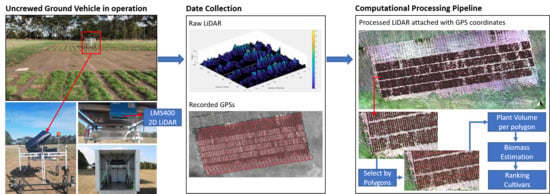
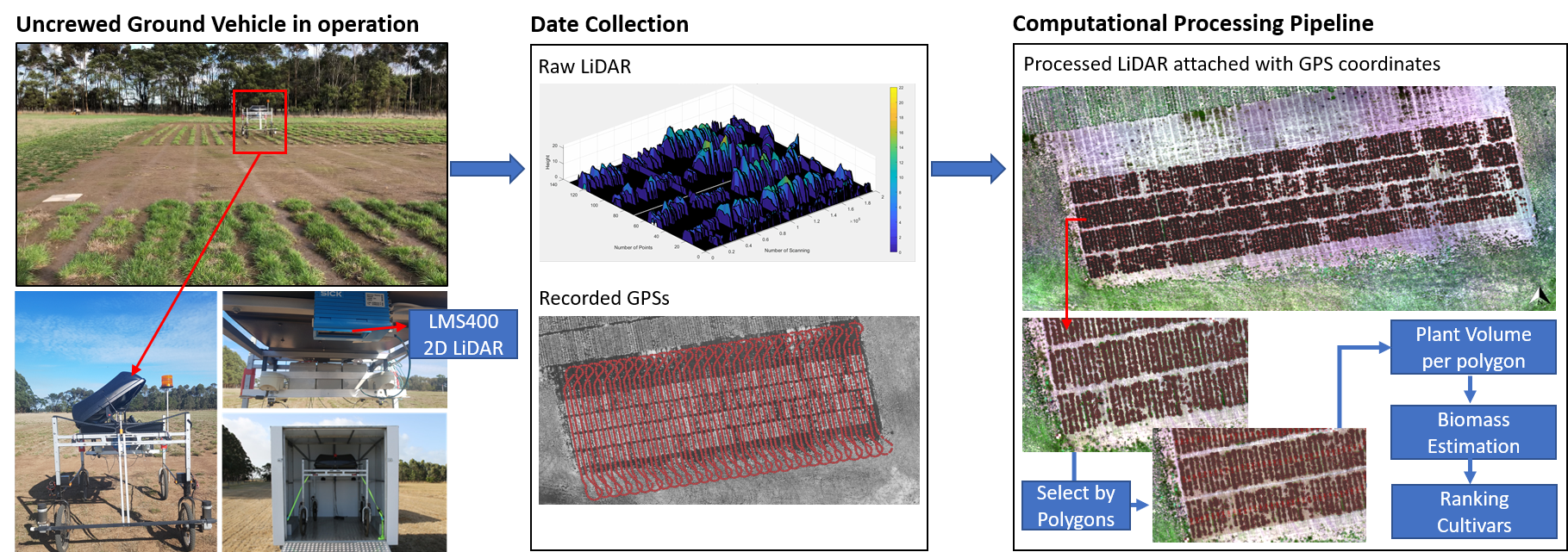
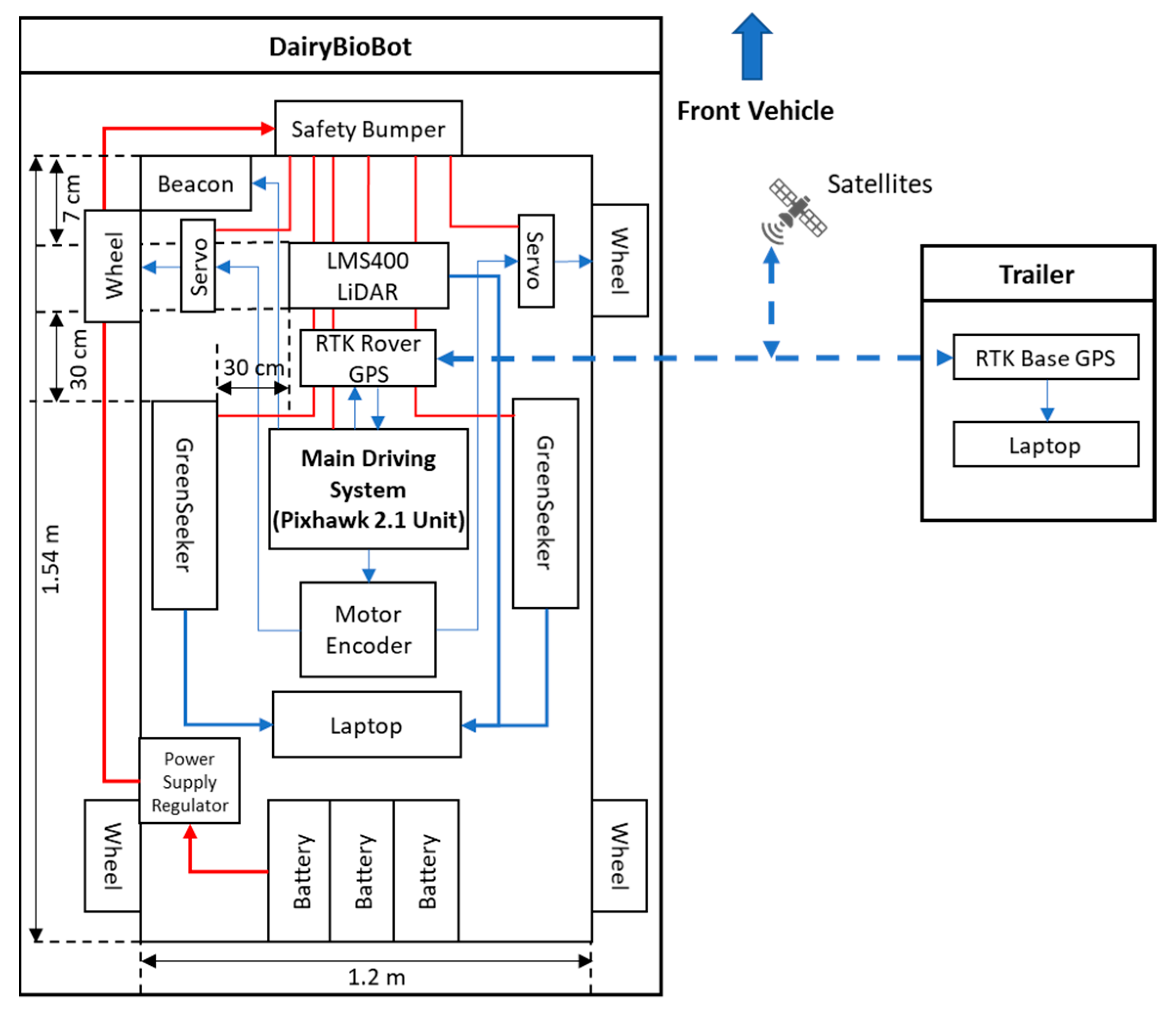
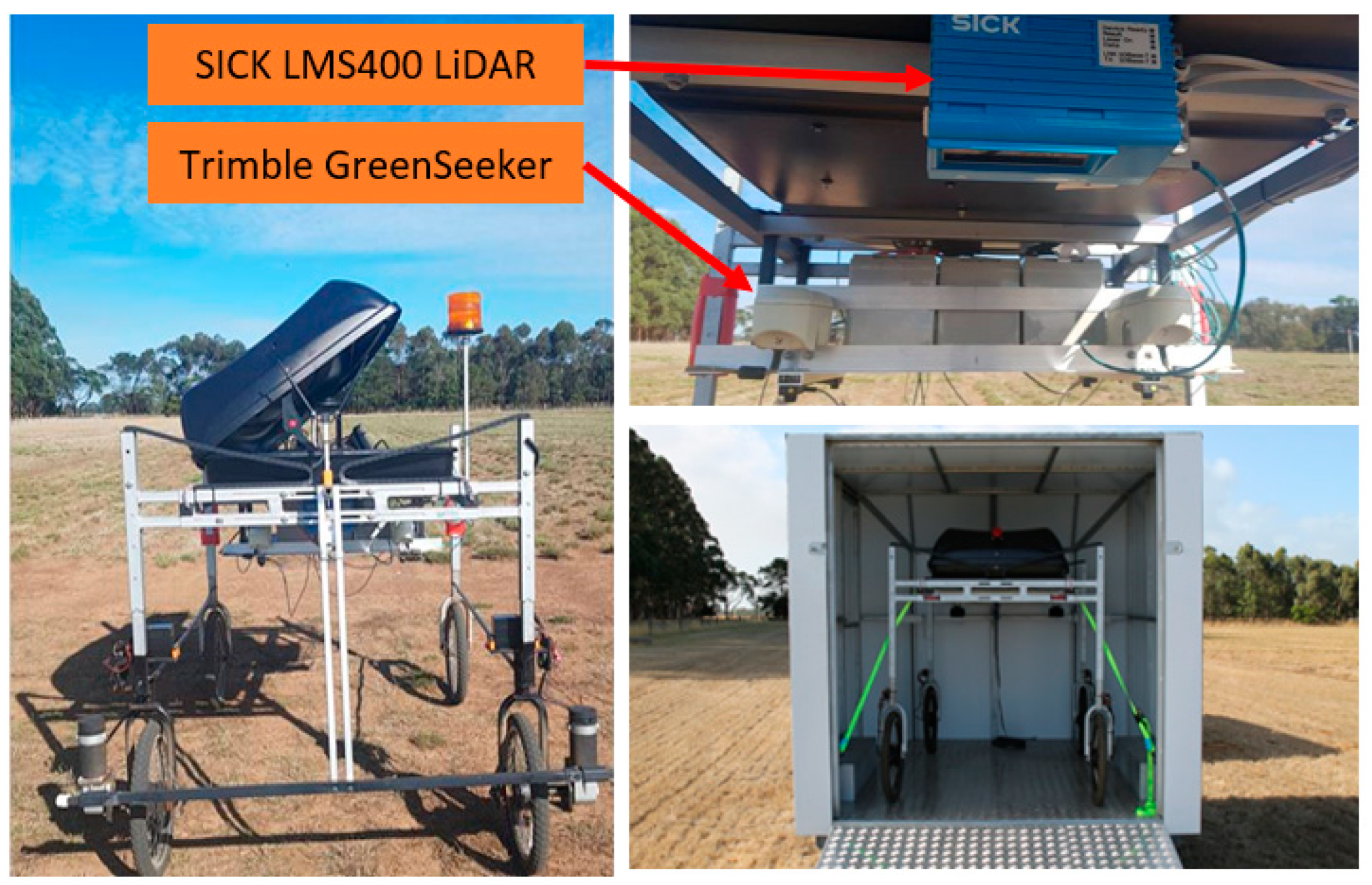
2.1. Unmanned Ground Vehicle (UGV)

The DairyBioBot, a UGV, was designed and purpose-built to monitor and assess the growth and performance of forages in experimental field trials. The prototyping of the DairyBioBot’s capability and performance was carried out in a perennial ryegrass field trial at the Agriculture Victoria Research Hamilton Centre, Victoria, Australia (Coordinates: −37.846809 S, 142.074322 E).

2.1.1. System Architecture Design

The DairyBioBot is a low-weight four-wheel system with front-wheel drive. The frame is made of aluminum alloy and can be adjustable (1000–1500 mm height), which is low-cost, durable, and flexible for further modification and replacement. The drive system utilizes electric 320 W 24 V 128 RPM 25 n-M drive worm motors (Motion Dynamics Australia Pty Ltd, Wetherill Park, NSW, Australia) for each front wheel independently, while electronic SUPER500 high-torque metal 12 V to 24 V 500 kg/cm (Happymodel, Quzhou, Zhejiang, China) servos steer the vehicle. The two drive motors were controlled by RoboClaw 2 × 30 A motor controllers (Basicmicro Motion Control, Temecula, Canada). The UGV is equipped with the Pixhawk 2.1 Cube flight control unit (Hex Technology Limited, ProfiCNC, PX4 autopilot, and Ardupilot; http://www.proficnc.com/) as a core part of the main driving system to connect and control all the electrical and driving components. The unit enables point-and-click waypoint entry, heads-up display, and telemetry data link as well as hosting an array of safety features such as geofence and failsafe systems. For precise navigation and tracking, the Here+ V2 RTK GPS kit (including Here+ RTK Rover GPS module and Here + RTK Base GPS and USB Connector module) was used. The Here+ V2 is a small, light, and power-efficient module with a high navigation sensitivity (167 dBm) and has a concurrent reception of up to three augment GNSS systems (Galileo, GLONASS, and BeiDou) incorporated with a Global Position System (GPS). This module can provide centimeter-level positioning accuracy with a speed measurement of up to 5 Hz. The Here+ RTK Rover GPS module was connected to the Pixhawk unit at the GPS connector on the DairyBioBot, while the Here+ RTK Base GPS and USB module was connected through the laptop USB port at the base station. To ensure smooth and accurate turns, a motor encoder unit programmed an appropriate wheel rotation for each front wheel and is configurable to the vehicle’s selected track width. The LMS400 2D LiDAR (SICK Vertriebs-GmbH, Germany) unit was used to precisely measure distances and contours. The width track of DairyBioBot was set at 1.2 m long to capture two rows of perennial ryegrass planted 60 cm apart. The LMS400 LiDAR unit was placed centrally under the roof-box and mounted 7 cm behind the front wheels to ensure that the field of view (FOV) of the LMS400 is not affected by the wheels. This FOV footprint of the LMS400 can be adjusted through adjusting the height of the DairyBioBot. Two Trimble GreenSeekers were mounted 30 cm behind and 30 cm offset to the left and right of the LMS400 unit and were used to measure NDVI. The FOV of each GreenSeeker is wider than a single plant, making it suitable for measuring a sward or plot rather than a single plant or single row. Captured data are transferred and stored on a Dell Latitude E6440 laptop (Dell, Round Rock, TX, US) for processing and analysis. For safety, a metal frame at the front acts as a safety bumper that immediately shuts down the DairyBioBot operation when it comes in contact with an object. A RS 236-127 12 V 2 W beacon (RS Components Pty Ltd, Smithfield, NSW, Australia) is also installed on the vehicle to indicate whether the vehicle is in operation. The Prorack EXP7 Exploro Roof Box (Yakima Australia Pty Ltd, Queensland, Australia) provides a waterproof space for storing sensors and hardware on the DairyBioBot. To reduce the overall weight of the vehicle, Drypower batteries have been used. Three IFR12-650-Y 12.8 V 65 Ah Lithium Iron Phosphate (Drypower, Australia; http://www.drypower.com.au/) rechargeable batteries were used to power the DairyBioBot’s operation and placed on the bedding frame at the back. The total weight of the UGV is 170 kg with three batteries and payload, as shown in Figure 1, which allows travel at the speed of 4.3 km/h (or 1.2 m/s) and up to 70 km on a full charge.

2.1.2. Trailer Design

As the DairyBioBot was designed to be deployed on different trials at different locations, the customized box enclosed trailer (shown in Figure 2) was designed as a secure housing for the DairyBioBot as well as a mobile base station for the RTK system. Through the telemetry data link installed in the trailer, the Pixhawk unit can be remotely controlled and transmits/receives data from/between the telemetry modules. One telemetry module was adapted to the Piwhawk unit via a TELEM port and another one is connected to a USB port of a Panasonic Toughbook CF-54 laptop (Panasonic, Osaka, Japan) at the base station. Mission Planner software was installed on the laptop at the base station to communicate with the Piwhawk unit through a telemetry data link.

The trailer can be connected to any appropriate tow vehicles, has a remote control to open/close the tailgate as a ramp for unloading/loading the UGV, and has stabilizing legs to stabilize the trailer when parked. The DairyBioBot is secured by a bedded position designed on the trailer and by additional ratchet straps attached to the trailer when traveling. The trailer is equipped with a solar charger PowEx PX-s20 system (Zylux Distribution Pty. Ltd., VIC, Australia) with two 12 V–24 V 20 A Solar Panels placed on the roof of the trailer and a 12–24 V 20 A Solar Regulator Battery Charger that is used to charge two Century C12-120XDA 12 V 120 Ah Deep Cycle (Century Batteries, Kensington, VIC, Australia) batteries on the trailer. These batteries were used to power the base station and additional accessories in the trailer and as a power source to charge the DairyBioBot, allowing for consecutive days of deployment without reliance on 240 V AC power. The Projecta 12 V 1000 W Modified Sine Wave Inverter (Brown & Watson International Pty. Ltd., VIC, Australia) is installed to convert 12 V DC from the Solar panels to 240 V AC power to have easy access and charge applications that required a 240 V supply, such as laptop and remote controller chargers. To maintain high-performance and long-life batteries, the Blue Smart 12 V/15 A IP65 Charger (Victron Energy B.V., Almere, The Netherlands) was used to charge all three batteries on DairyBioBot by providing a seven-step charging algorithm and a deeply discharged battery function at a low current; the charging status can be remotely checked by smart devices through a Bluetooth connection. Charging with solar power at the trailer avoids the need to place all this equipment on the UGV, thereby making the UGV lighter and smaller. In addition, consecutive charging and discharging reduce battery life and performance. The trailer was also equipped with a bench and chair to allow the operator to use the trailer as a workstation.

2.1.3. Navigation System

The mobile base-station fitted to the trailer requires a fixed-location to be surveyed prior to the deployment of the DairyBioBot unit to allow for RTK-GNSS navigation. The surveying procedure for the mobile base-station can be done either through RTKNavi version 2.4.3 b33 (Tomoji Takasu, Yamanashi, Japan; http://www.rtklib.com/) or the Mission Planner version 1.3.68 software (ArduPilot Development Team and Community; https://ardupilot.org/planner/). By connecting to the internet, the RTKNavi software with built-in algorithms can access the Continuously Operating Reference Station (CORS) network to provide a GPS location of the base station with an accuracy of up to 3 cm in a few hours [69]. Without requiring internet connection, Mission Planner can obtain a location from Here + RTK Base GPS and USB Connector module for an extended period and uses an algorithm to correct its occupied position accuracy. To achieve the same accuracy by RTKNavi, the process may require several days.

2.1.4. Driving Operation

The DairyBioBot can be operated both manually via a remote control FrSky Taranis X9D Plus 2019 (FrSky, Jiangsu, China) and automatically from a created mission, which is imported to Mission Planner software. As the DairyBioBot operates in a large area, we integrated an RFD 900+ modem (RFDesign Pty Ltd., Archerfield, QLD, Australia) associated with an Omni Outdoor Antenna High Gian Fiberglass Full Wave 915 MHz 6 dBi RP-SMA (Core Electronics, Adamstown, NSW, Australia) on the base station to extend the connection range to the DairyBioBot. For our row/plot field trial, we developed a specific program and graphical user interface to create missions from measured GPS points to navigate the DairyBioBot on specific paths through a field trial (Figure 3). High-accuracy GPS points for our row/plot field trials were obtained by a Trimble RTK GNSS receiver (Navcom SF-3040, Nav Com Technology Inc., Torrance, CA, USA), which can provide an accuracy of 2 cm. In our ryegrass trial, the aim was to be able to drive over two rows, make a turn, and then drive over the next two rows within the trial.

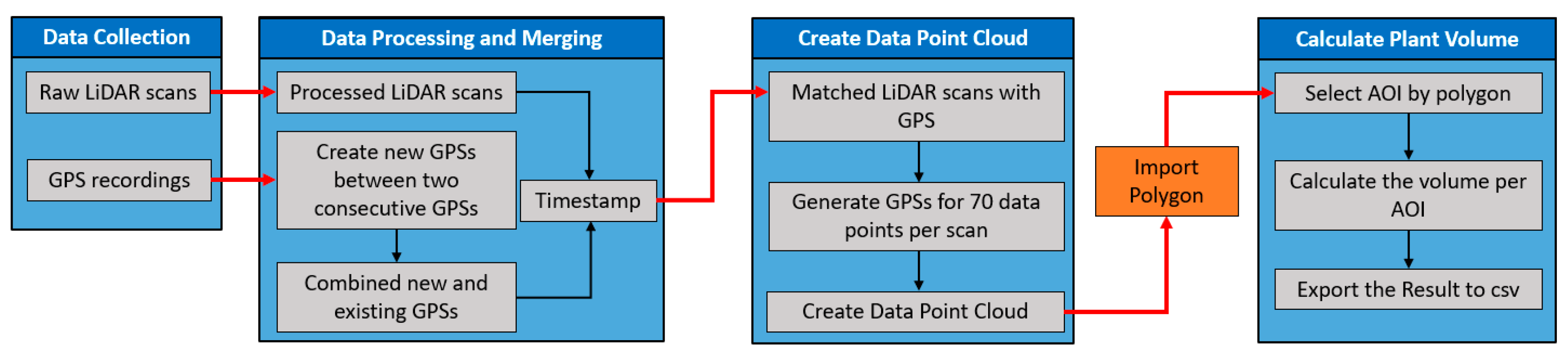
2.2. LiDAR Signal Reception and Processing

The scan frequency and the angular range were set at a maximum of 500 Hz and from 55° to 123°, respectively, according to the manufacturer’s recommendation. With the deployment of DairyBioBot over the ryegrass row trials, the LiDAR was mounted at a distance of 1.127 m to the ground level to cover a width of 1.578 m (or to cover two rows per scan). At a scan resolution of 1°, each scan creates 70 data points that measure the distances to a zero point (which is at the center of the LMS400 LiDAR unit) on the respective scan angle. The measured distance values are presented in polar coordinates depending on the scan range (Figure 4). The scan range can be up to 3 m, but the detectable area is at least 70 cm away from the LMS400 unit. To convert from a polar to a cartesian coordinate system to present objects as compared to the ground level, the converted distance values and their position to the zero point per scan can be calculated with the following formula:

$$h_{\alpha }=\left(h_0-\cos \left(\alpha \right)\ast d_{\alpha }\right),$$

(1)

$$x_{\alpha }=\sin \left(\alpha \right)\ast d_{\alpha },$$

(2)

where $h_{\alpha }$ is the converted height value on scan angle $\alpha$ (in mm), $h_0$ is the measured distance from the LMS400 LiDAR sensor to the ground level (mm), $\alpha$ is the scan angle and $d_{\alpha }$ is the measured distance to the zero point on respective angular scan $\alpha$ (in mm), and $x_{\alpha }$ is a position of $d_{\alpha }$ to the zero point on the horizontal axis (mm).

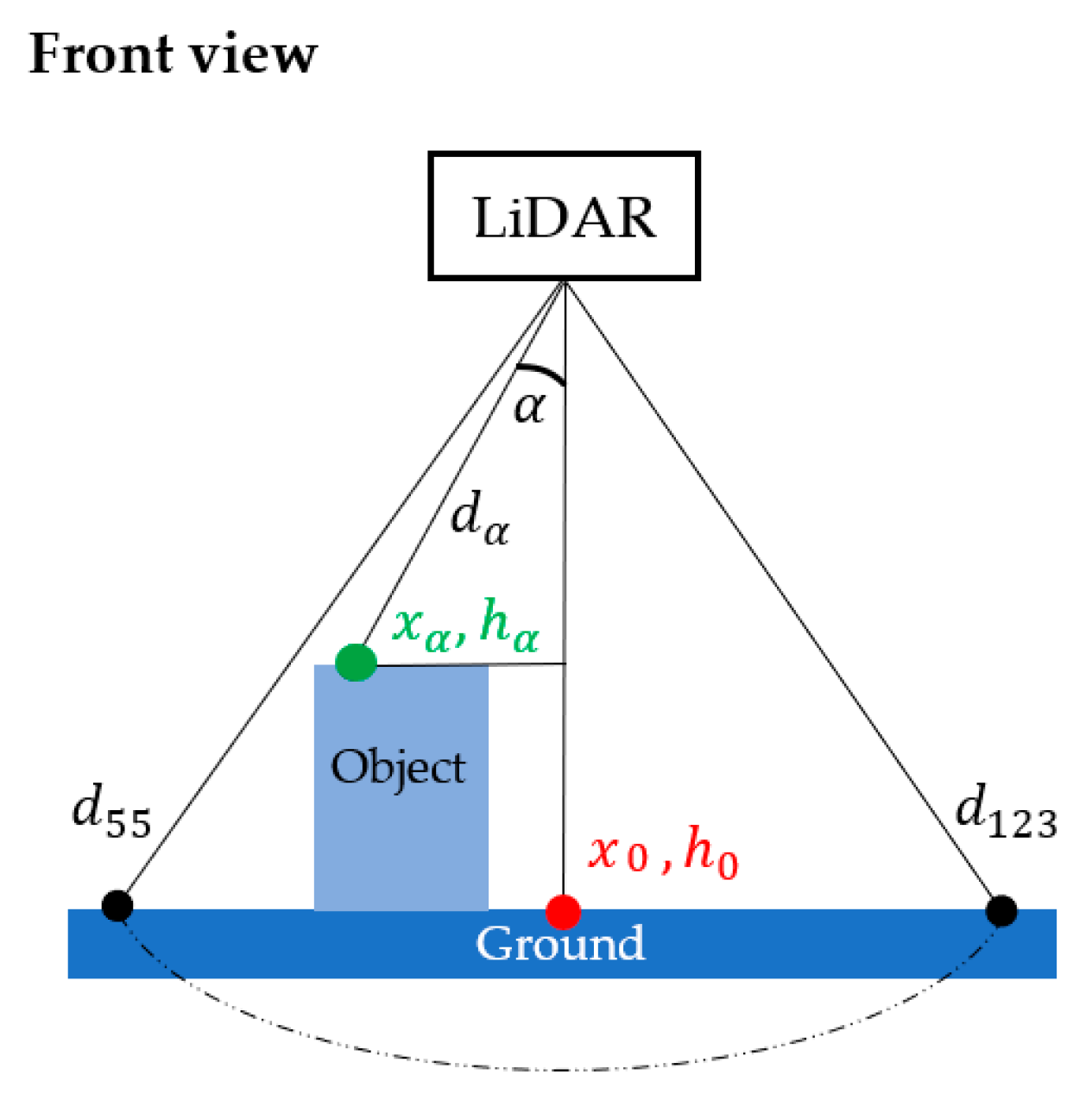
2.3. Estimated LiDAR Volume Equation

Each scan creates a contour of an object from 70 converted height values. We can estimate the volume of an object by measuring the area of scans and width between each scan, which is constant at constant driving speed. Therefore, the volume of an object can be calculated as:

$$V_{object}={\sum }_1^N\left(\int f(x,y)dxdy\ast \Delta z\right),$$

(3)

where $V_{object}$ is the volume of the object, $f\left(x,y\right)$ is the area of the object occupied in each scan, $\Delta z$ is a distance between each scan, and N is the number of scans.

2.4. LiDAR Data Validation in Experiment

A data validation experiment was designed using a rectangular cardboard box to define the accuracy and quality of LiDAR measurements recorded during driving. A rectangular cardboard box volume can be calculated as:

$$Volume=Width\ast Height\ast Length.$$

(4)

Five differently sized boxes were placed in a line with clear gaps (Figure S1). The DairyBioBot was manually driven over the boxes to capture LiDAR data at a speed of 4.3 km/h (1.2 m/s). The LiDAR data was then processed as described above and visualized in a three-dimensional (3D) view in MATLAB R2019b (The MathWorks Inc., Natick, MA, USA; https://www.mathworks.com/) software. The MATLAB Data Tip tool was used to measure dimensions, which were then compared to ruler measurements. General linear regression was used to estimate the coefficient of determination between the two-volume measures and is presented in the first part of the Results section.

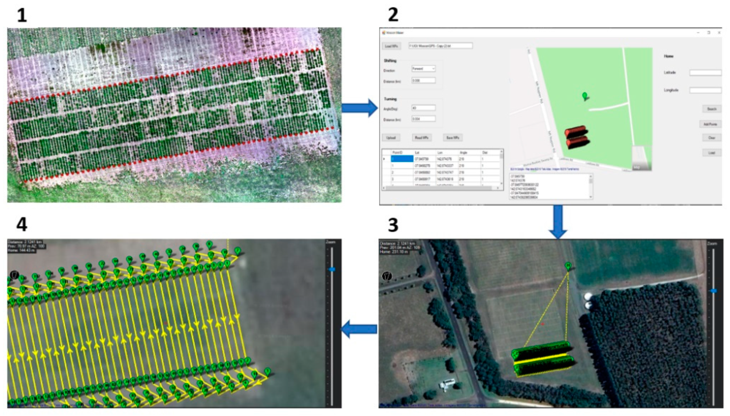
2.5. LiDAR Mapping Method

The relating of the LiDAR data to a georeferenced map required the interpolation of georeferenced coordinates to each data point in the 3D data point cloud. The LMS400 LiDAR does not have an integrated GPS unit and relies on an independent GPS unit and post-processing. Therefore, we have developed a data processing pipeline that matches the LiDAR data with GPS data recorded by Here+ V2 RTK GPS kit based on their timestamps to create a data point cloud to calculate the plant volume per row/plot (Figure 5).

After data collection, raw LiDAR data were processed using Equations (1) and (2) with a 5 cm aboveground threshold, which is the common ryegrass harvest height. The GPS frequency is low at 5 Hz (5 scans/s), and only LiDAR data with the exact same timestamp as GPS could be matched. Therefore, the GPS coordinates for the LiDAR data between two consecutive GPS points must be inferred. The time and distance traveled are known from the two consecutive time points and the initial bearing angle between the two points was calculated from the first time point to the next time point by the forward Azimuth formula to define the vehicle’s direction. Field testing revealed that the bearing angle had an offset of 10° compared to the actual direction, therefore, all initial bearing angles were subtracted by 10°. A number of assumed GPS points were then defined by dividing the elapsed time between two GPS points by the LiDAR scan rate (2 ms/scan). The new GPS coordinates associated with each timestamp were inferred based on the calculated distance and initial bearing angle in a loop for a number of assumed GPS points in which the timestamp was taken from the first point of two consecutive points and then increased by the scan rate (2 ms) on each iteration. The new GPS points were then appended to the existing set. Based on the timestamp, the processed LiDAR scans were merged with the GPS data. When the bearing angle was greater than 345° and less than 351° (north by west direction in the 32-point compass rose) in the mission, it signified the turning of the DairyBioBot to drive over the next two rows, and thus the LiDAR scans were flipped to account for the change in orientation. To simplify the processing, the bearing angle of all scans was fixed at 167° (south by east direction), as all the scans were in the same orientation.

In creating a data point cloud step, GPS coordinates for each scan were converted to the coordinate reference system World Geodetic System 1984 (WGS)/Universal Transverse Mercator (UTM) zone 54S. Each LiDAR scan was annotated with GPS coordinates for a single point per scan by applying distances of north and east directions, fixed bearing angle, and GPS coordinates of a scan. There was a 20 cm distance between the mounting position of the GPS and LMS400 sensor on the DairyBioBot, so the east distance is set to 0.2 m in the script. For the north distance, an array for 70 points was calculated based on the scan width of the LMS400 LiDAR to the ground. All the resulting single points in each scan were then extracted to create a data table with three columns: UTMX (easting), UTMY (northing), and height.

The field trial was exactly sown allowing the rectangular polygon of each row to be drawn manually on an aerial image of the trial via Add rectangular from 3 Points tool in the QGIS 3.4.15 software (QGIS.org(2020). QGIS Geographic Information System. Open Source Geospatial Foundation Project; http://qgis.osgeo.org). This enables the selection of areas of interest (AOI), such as rows and columns. Polygons were classified by the row and plot identity (ID) numbers and saved as a shapefile file with the projected coordinate system of EPSG: 32754–WGS 84/UTM zone 54 S. The merging conditions were set to within and intersect with polygon to optimally select the LiDAR points per polygon to calculate the volume per row. The volume per plot was calculated as the sum of its three rows. The data processing pipeline was performed with the Python programming language (Python Software Foundation, Python Language Reference, version 3.7; http://www.python.org/).

2.6. Field Experiment

The field trial was located at the Agriculture Victoria Hamilton SmartFarm, Hamilton, Victoria, Australia (Coordinates: −37.846809 S, 142.074322 E). The trial was established in June 2017 with 18 varieties of perennial ryegrass each grown in 7 to 11 replicate plots and was designed as a row/plot field trial, resulting in a total of 160 plots (480 rows), laid out in a 4 plot × 40 plot configuration. Each plot was 4 m long and 1.8 m wide and consisted of 48 plants in three rows each with 16 plants. A gap between rows was 60 cm. The gap between the top of each row was 1 m. Plants were harvested when the plots were at the reproductive stage in December 2019.

2.6.1. Ground-Truth Sampling

The biomass of all plots was collected by a destructive harvest method using a push mower. The cut level was set at 5 cm above the ground. The mower was a 21″ self-propelled lawn mower (Model: HRX217K5HYUA; Engine capacity—190 cc; Honda Motor Co., Ltd., Tokyo, Japan). Each row was collected separately. All the ground-truth samples were weighed for FM to estimate their relationship with plant volume measured from LiDAR.

2.6.2. Aerial Images Captured by UAV

DJI Matric 100 (DJI Technology Co., Shenzhen, China) UAV mounted with a RedEdge-M (MicaSense Inc., Seattle, WA, USA) multispectral camera was used to capture aerial images of the field trial. Pix4DCapture software (Piz4D SA, Switzerland; https://www.pix4d.com/) was used to generate automated flight missions based on the areas of interest. Image overlap was set at 75% forward and 75% sideways. The UAV was flown at 30 m above ground level with a speed of 2.5 m/s (9 km/h) on a flight path specified by the planned mission. The RedEdge-M multispectral camera was mounted under the UAV at an angle of 90° to the direction of travel and pointing directly downward. To ensure capturing high-quality images with UAV configurations, the RedEdge-M camera picture trigger is set on fast mode with Ground Sample Distance (GSD) 2.08 cm per pixel and auto white balance. To calibrate the reflectance values of the acquired images, radiometric calibration tarps (Tetracam INC. Chatsworth, CA, USA) with five known reflectance values (3%, 6%, 11%, 22%, and 33%) was placed on the ground at the corner of the trial during image capturing. Orthomosaic images of each multispectral band were created in the Pix4D mapper 4.2.16 software (Pix4D SA, Switzerland; https://www.pix4d.com/) following the recommended Pix4D processing workflow. As a part of the image processing in the Pix4D software, the ground control points (GCPs) were required for the georectification of the orthomosaic final image. Six GCPs were placed within the field trials (four at the corners and two inside at the center of the trial) and measured by a Trimble RTK GNSS receiver (Navcom SF-3040, Nav Com Technology Inc., Torrance, CA, USA). The output image was set to the Coordinate Reference System (CRS) WGS 84 54 S.

2.6.3. LiDAR Data Captured by the DairyBioBot

The SICK LMS400 LiDAR was set up as discussed in the previous section and data were stored on a laptop onboard the DairyBioBot. Here+ V2 RTK GPS kit was set to record GPS data at a frequency of 5 Hz and all GPS recordings were automatically saved by the Mission Planner software on the laptop at the base station. A created mission made by the developed Mission Maker application was imported to the Mission Planner software to navigate DairyBioBot in this field trial with total travel distance of 2.1 km. The DairyBioBot was manually controlled from the trailer to the field trial site and waited until an RTK Fixed mode to be acquired before starting the automated mission. This RTK Fixed mode indicates that the DairyBioBot has entered the RTK mode, which can provide a better signal strength and a higher positioning accuracy. Once RTK Fixed mode was acquired, the automated mission was started in Mission Planner and the DairyBioBot started driving the guided planned mission and record data, as indicated in the next result section with a constant speed of 4.3 km/h. Recorded GPS points were extracted from the Mission Planner logging file and converted to CRS EPSG: 4326–WGS 84. This allowed for the visualization of the GPS recordings of the DairyBioBot on the aerial image captured from the DJI M100 (DJI Technology Co., Shenzhen, China) UAV on the same date on the QGIS software. Additionally, the position error and average position error are used to evaluate the accuracy of autonomous navigation and are determined by formulas described in [70]. The cross-track error (distance) of recorded GPS points along each two-row path were also calculated following the formula in the papers [71,72,73] to verify the trajectory accuracy. All the LiDAR and GPS recordings were processed and analyzed through our developed pipeline to calculate the plant volume per row/plot.

3. Results

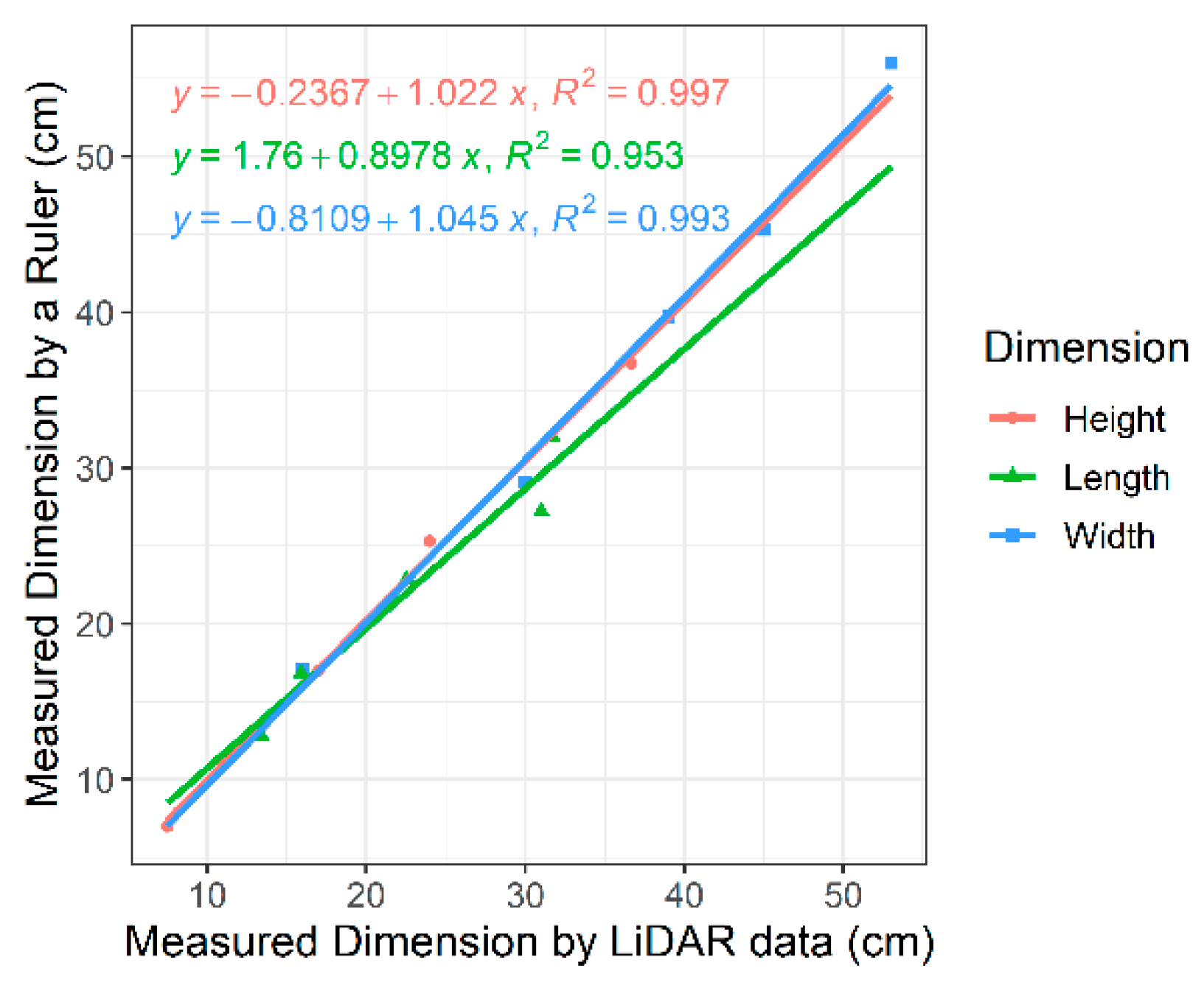
3.1. Validation Experiment Result

Our validation on five cardboard boxes demonstrated highly accurate measurements of all three dimensions of the objects under our setting (Figure 6): the R² score of fitting a linear regression between the actual size and the LiDAR-measured size in the X (width), Y (height), and Z (length) dimensions was 0.993, 0.997, and 0.953, respectively. As a result, the volumes estimated from the LiDAR measurements were about 98% of the actual volumes on average, with the standard deviation of differences at 885.23 cm³ and the R² score of fitting a linear regression for the volume across the five objects at 0.997. The slight difference between the actual volumes and the measured volumes was potentially caused by subtle experimental errors such as equipment fluctuation due to the rough surface.

3.2. Autonomous Driving Performance

The DairyBioBot successfully navigated the field trial without human control, as demonstrated by the aerial image with recorded GPS points in Figure 7. At a speed of 4.3 km/h, the DairyBioBot has traversed the whole trial traveling up and down 60 times across pairs of rows within approximately 40 min. From Figure 8, the position error at 120 planned and recorded GPS points ranged up to a maximum 0.45 cm, while most were less than 0.3 cm. The average position error was 0.175 cm that demonstrates a high accuracy of trajectory tracking in entering the two-row paths. Within the two-row paths, the mean cross-track error was smaller (6.23 cm) in comparison of outlier points (a range of 12.5 cm) of the path. The path was planned in the Mission Maker application, and recorded GPS points of the DairyBioBot were recorded consistently and have an adequate amount of coverage by a mean 41 points with approximately four outlier points (Figure 9) for a 17.8 m distance path throughout the trial to allow for further processing.

3.3. LiDAR Mapping Performance

The LiDAR data were appropriately matched to GPS points to map the ryegrass rows and plots in the field trial (Figure 10). Most of the plant canopy was covered by LiDAR data points, with some plants shorter than 5 cm being excluded. A clear gap is visible between rows, which would allow for the drawing of polygons from the LiDAR data itself if desired or an aerial image in this case (Figure S2). Hence, the LiDAR data of rows can be correctly selected by created polygons with row ID numbers to calculate the plant volume.

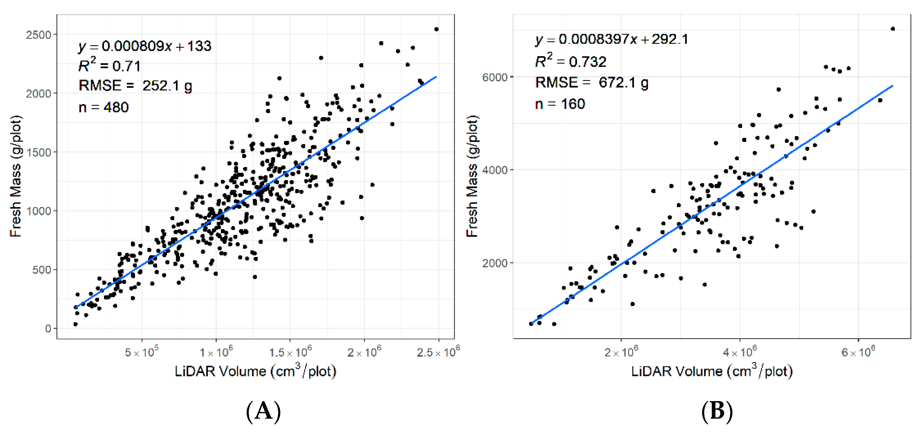
3.4. Correlation between LiDAR Plant Volume and Biomass

The data were captured in December 2019 during the summer season when the plants were flowering (Figure 11). A variation in biomass was observed that included vegetative biomass, stems, and seed heads. The R² between the LiDAR-derived volume and fresh biomass across for rows was 0.71 and for plots was 0.73. Higher R² may be possible when plants are not flowering.

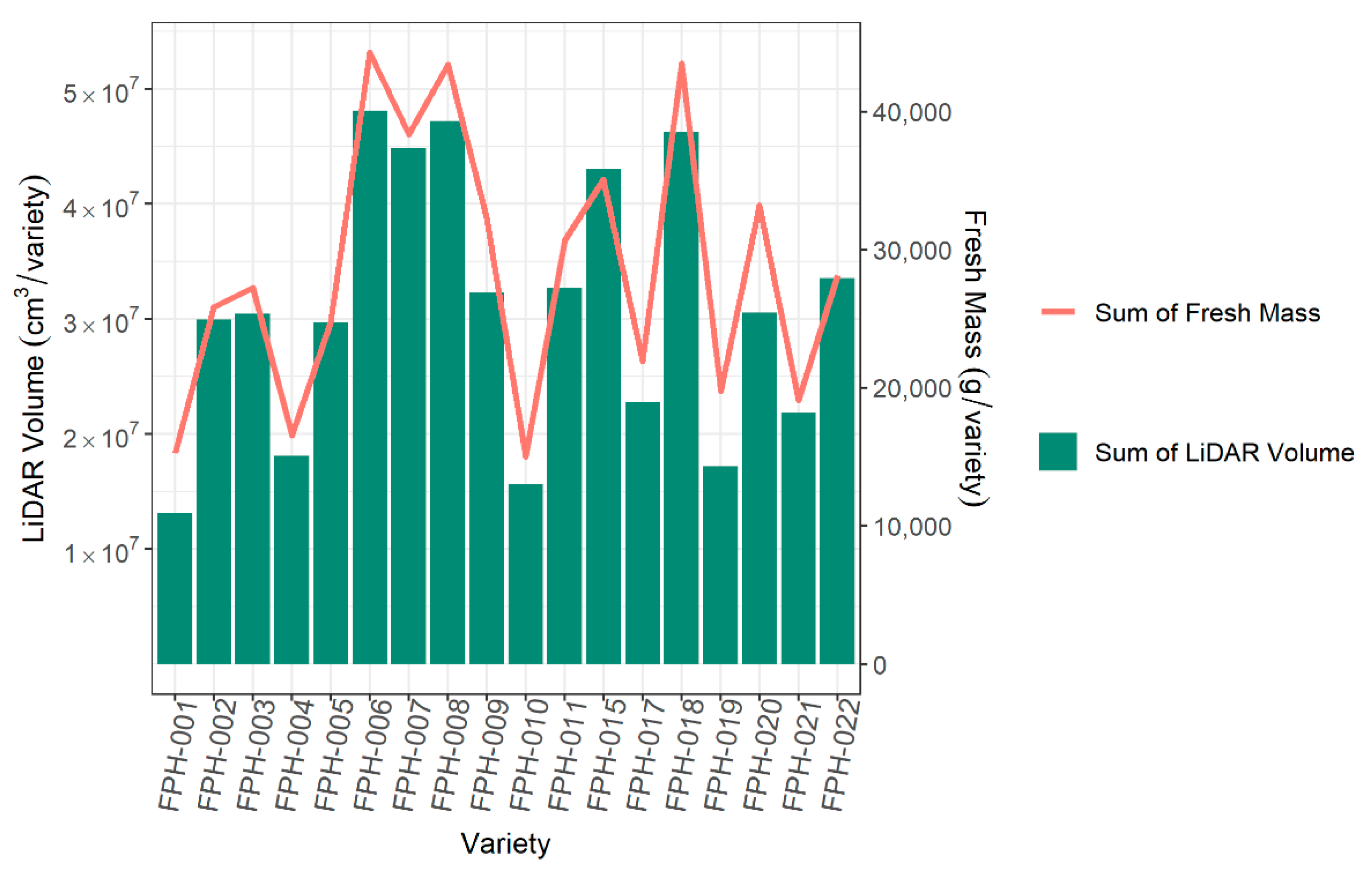
3.5. Ranking Varieties Based on LiDAR Plant Volume Versus Biomass

A key aim of using high-throughput phenomics is to rank lines or varieties. The ranking of varieties based on LiDAR was very similar to that from fresh biomass (Figure 12). Therefore, the ranking order of LiDAR plant volume can be used to identify top cultivars and potentially replace conventional biomass as a phenotype.

4. Discussion

In this paper, we have demonstrated the capability of the developed UGV DairyBioBot and a data processing pipeline as a non-destructive, effective, and high-throughput phenotyping platform to assess the biomass of perennial ryegrass using LiDAR sensor technology in field conditions. This platform could replace conventional methods which can be imprecise, time-consuming, and/or required destructive harvests for estimating FM and DM accumulation. The DairyBioBot had excellent autonomous navigation through the row field trial with a 60 cm gap between rows and capturing the data of 480 rows (or 160 plots) within 40 min. With the ability to cover 70 km by three large capacity batteries, it can repeat the mission more than 30 times on one full charge and more after recharging from solar power. Although the set-up cost of the autonomous vehicle is greater than mounting sensors on existing ground-based crewed vehicles, the DairyBioBot has the great advantage of having a low operational cost for long-term deployment, and this would also be true if the sensors were mounted on pre-existing autonomous vehicles. In contrast, conventional methods can accrue a significant amount of time and labor costs depending on the level of assessment and trial size. For the row assessment, a person using a visual score can take up a half minute per row including scoring and recording, and that can result in up to 4 h working in the field with 480 rows. Even more for actual biomass, the time taken for each row using manual harvesting is approximately 7 min from cutting and bagging to weighing. Furthermore, in the breeding of new forage cultivars, multiple measurements across years are needed to evaluate the biomass performance in response to the season and climate variability. Substantial time and cost savings can be realized by using the DairyBioBot in place of a visual score or destructive methods, especially in larger field trials. Importantly, rich high-resolution LiDAR data from screening hundreds of rows provides more an accurate biomass estimation than a simple ranking of the visual score. Thus, the DairyBioBot can replace the conventional and destructive methods to assess the in-field biomass of a large population of perennials in modern genomic selection programs.

With the current design, DairyBioBot has a total weight of 170 kg, which is lighter than the crewed ground vehicles that are currently in use. Soil compaction has been identified as an issue in UGVs used for weed control in crops [20,74] when the minimum weight was around 300 kg [29,32] due to their robust structure and payload, as they carried weeding equipment along with sensing and self-charging systems. However, this lightweight structure with small bicycle wheels and without rugged wheels/shock absorbers limits the ability of the DairyBioBot to drive on rough and very wet terrains. Nevertheless, these conditions are not common in breeding trials. Another advantage of the DairyBioBot is that the frame can be adjusted to increase the resolution of plant architecture during plant growth and at various ages. Especially for grass species, vegetative parts can vary greatly in height due to plant growth and reproductive development. For these reasons, this design of DairyBioBot is suited for biomass estimation in ryegrass species sown in field trials.

The use of remote sensing is rapidly emerging for measuring and predicting biomass in plant science [75,76,77]. A wide range of proximal and optical sensors was used to estimate the biomass trait in field conditions [78,79]. Despite satellites effectively capturing large-scale areas, their resolution is not high enough to be suitable for phenotyping single-plant or row-based field trials. In breeding programs, field trials are usually designed as spaced-planted single plant trials, row trials, and plot or sward trials to monitor and evaluate each cultivar’s performance. For this configuration, high-resolution proximal sensors are required to ensure accurate measurement at different levels. Several studies in perennial ryegrass have been conducted to estimate in-field biomass [80]. Using an ultrasonic sensor to measure plant height, the estimated correlation between plant height and biomass at a single plant level varied from R² = 0.12 to 0.65 across seasons [39] and from 0.61 to 0.75 at the sward level [81]. The ultrasonic sensor measures the distance to a target by measuring the time between the emission and reception of ultrasonic waves. An echo in reflecting a target mainly depends on the surface of a target. As ultrasonic sensors have low scan frequencies that may not be suitable at higher driving speed, this can result in a sparsity of measured points and inaccurate measurements. The NDVI extracted from a UAV multispectral camera has been shown to have a moderate to good correlation with biomass with R² = 0.36 to 0.73 at the individual plant level [39]. Similarly, at the row plot level, the R² value of the NDVI and the biomass ranged from 0.59 to 0.79 [41]. However, the high variation in the correlation can be explained by the effect of the saturation of the NDVI value for high-density vegetative at late growth stages. To overcome the limitations of these methods, plant height and NDVI were combined and incorporated with predictive models to achieve a more robust R² [39,82,83]. In this study, the use of LiDAR on a UGV resulted in a similar correlation to those previously reported between plant volume and FM at both the row and plot-level (R² = 0.71 and 0.732, respectively). The R² on the plot level was slightly higher than in another study using LiDAR on a ground-based mobile vehicle where an R² of 0.67 was achieved on a December harvest [13]. It is necessary to note that the data was presented in this study during the reproductive phase of growth, which would have included vegetative biomass and flower heads. In the flowering period, the plant canopy creates a great complexity of plant structure, including a mixture of leaves and tiller with flowering heads. Overall, our results indicate that standalone LiDAR plant volume can be used to predict biomass for perennial ryegrass row and plot trials.

Although previous studies in perennial ryegrass have reported good results, data acquisition was generally via manual to semi-automated systems. Plant height was collected by manually driving the ground-based vehicle through all the rows/swards [39,81]. Ground-based vehicles are more familiar and potentially simpler to use and operate for plant breeders, farmers, and research scientists. However, manual methods require a large amount of time and labor depending on the field trial size. Human driving can also result in low data accuracy due to variations in speed and data entry errors. The use of UAVs offers an effective powerful approach that can rapidly produce multispectral images of large trials in a short amount of time. Nevertheless, image processing requires several steps (e.g., data importation, calibration, and processing; accurate georeferencing; and quality assessment) that can be time-consuming [84,85]. NDVI is generally calculated as the average NDVI value per measured area unit (e.g., within a polygon), which will include non-plant areas or soil. LiDAR data avoids these shortcomings, as it simultaneously provides accurate plant area and volume. In this study, the rectangular polygon of rows/plots was manually drawn to select LiDAR data within a polygon. This method is simple and suitable for a large object such as a row or a plot. Additionally, the polygons are drawn once at the beginning of the trial and are used until the trial is terminated, which in breeding can be up to 5 years. However, the definition of a polygon is not strictly necessary in LiDAR processing, as a polygon of rows/plots can be automatically constructed from the LiDAR data. The automated polygon detection requires more time in developing a proper algorithm and processing data to correctly detect each row/plot. Further development of this approach would be helpful to speed up the processing and remove the importation of manual polygons. An integrated, manually operated, semi-automated system was developed by Ghamkhar et al. [13] and has been used to measure the plant volume of single rows in an effective manner to estimate in-field biomass. Solutions that are not fully automated require more labor, which makes the successful scaling up to large field trials difficult. Fully automated systems offer a promising opportunity in agriculture that provides reliable high-resolution data, enhances data collection ability, and significantly reduces time-consuming costly operation and human involvement [86,87].

5. Conclusions

To the best of our knowledge, the DairyBioBot is the first UGV that has been designed and developed to autonomously measure the plant volume of perennial ryegrass. It is a completely automated high-throughput system to estimate biomass under field conditions capable of autonomous driving guided by real-time GPS. The initial results showed a good estimated correlation with biomass at the row and plot level, even when captured in the flowering period. In comparison with the observed R² in previous studies, the LiDAR data captured with the DairyBioBot provided a similar or more accurate measurement of biomass. The estimated R² id promising but will require further improvement and more understanding of the key influencing factors. The data processing pipeline has connected LiDAR and GPS data taken with two different sensors at different frequencies. The further development of the DairyBioBot will optimize the data collection and analysis with minimal human effort. The autonomous nature of the DairyBioBot results in a large reduction in the labor requirement for phenotyping, allowing for scaling up to larger trials and potentially remote locations through the use of a lockable base station trailer. The DairyBioBot has accurately assessed in-field biomass for perennial ryegrass, and further development may allow its use for biomass estimation for other pasture species.

6. Patents

This section is not mandatory but may be added if patents result from the work reported in this manuscript.

References

1. Wilkins, P.W. Breeding perennial ryegrass for agriculture. Euphytica 1991, 52, 201–214. [Google Scholar] [CrossRef]
2. Forster, J.; Cogan, N. Pasture Molecular Genetic Technologies—Pre-Competitive Facilitated Adoption by Pasture Plant Breeding Companies; Meat and Livestock Australia Limited: Sydney, Australia, 2015; Available online: https://www.mla.com.au/contentassets/15eeddae0eee4ea88af7487e7c203b7a/p.psh.0572_final_report.pdf (accessed on 19 August 2020).
3. Li, H.; Rasheed, A.; Hickey, L.T.; He, Z. Fast-Forwarding Genetic Gain. Trends Plant Sci. 2018, 23, 184–186. [Google Scholar] [CrossRef] [PubMed] [Green Version]
4. McDonagh, J.; O’Donovan, M.; McEvoy, M.; Gilliland, T.J. Genetic gain in perennial ryegrass (Lolium perenne) varieties 1973 to 2013. Euphytica 2016, 212, 187–199. [Google Scholar] [CrossRef] [Green Version]
5. Harmer, M.; Stewart, A.V.; Woodfield, D. Genetic gain in perennial ryegrass forage yield in Australia and New Zealand. J. N. Z. Grassl. 2016, 78, 133–138. [Google Scholar] [CrossRef]
6. Reynolds, M.; Foulkes, J.; Furbank, R.; Griffiths, S.; King, J.; Murchie, E.; Parry, M.; Slafer, G. Achieving yield gains in wheat. Plant Cell Environ. 2012, 35, 1799–1823. [Google Scholar] [CrossRef]
7. Pardey, P.G.; Beddow, J.M.; Hurley, T.M.; Beatty, T.K.M.; Eidman, V.R. A Bounds Analysis of World Food Futures: Global Agriculture through to 2050. Aust. J. Agric. Resour. Econ. 2014, 58, 571–589. [Google Scholar] [CrossRef] [Green Version]
8. O’Donovan, M.; Dillon, P.; Rath, M.; Stakelum, G. A Comparison of Four Methods of Herbage Mass Estimation. Ir. J. Agric. Food Res. 2002, 41, 17–27. [Google Scholar]
9. Murphy, W.M.; Silman, J.P.; Barreto, A.D.M. A comparison of quadrat, capacitance meter, HFRO sward stick, and rising plate for estimating herbage mass in a smooth-stalked, meadowgrass-dominant white clover sward. Grass Forage Sci. 1995, 50, 452–455. [Google Scholar] [CrossRef]
10. Fehmi, J.S.; Stevens, J.M. A plate meter inadequately estimated herbage mass in a semi-arid grassland. Grass Forage Sci. 2009, 64, 322–327. [Google Scholar] [CrossRef]
11. Tadmor, N.H.; Brieghet, A.; Noy-Meir, I.; Benjamin, R.W.; Eyal, E. An evaluation of the calibrated weight-estimate method for measuring production in annual vegetation. Rangel. Ecol. Manag. J. Range Manag. Arch. 1975, 28, 65–69. [Google Scholar] [CrossRef]
12. Huang, W.; Ratkowsky, D.A.; Hui, C.; Wang, P.; Su, J.; Shi, P. Leaf fresh weight versus dry weight: Which is better for describing the scaling relationship between leaf biomass and leaf area for broad-leaved plants? Forests 2019, 10, 256. [Google Scholar] [CrossRef] [Green Version]
13. Ghamkhar, K.; Irie, K.; Hagedorn, M.; Hsiao, J.; Fourie, J.; Gebbie, S.; Hoyos-Villegas, V.; George, R.; Stewart, A.; Inch, C.; et al. Real-time, non-destructive and in-field foliage yield and growth rate measurement in perennial ryegrass (Lolium perenne L.). Plant Methods 2019, 15, 72. [Google Scholar] [CrossRef] [PubMed]
14. Zhao, C.; Zhang, Y.; Du, J.; Guo, X.; Wen, W.; Gu, S.; Wang, J.; Fan, J. Crop Phenomics: Current Status and Perspectives. Front. Plant Sci. 2019, 10, 714. [Google Scholar] [CrossRef] [Green Version]
15. Araus, J.L.; Kefauver, S.C.; Zaman-Allah, M.; Olsen, M.S.; Cairns, J.E. Translating High-Throughput Phenotyping into Genetic Gain. Trends Plant Sci. 2018, 23, 451–466. [Google Scholar] [CrossRef] [PubMed] [Green Version]
16. Haghighattalab, A.; González Pérez, L.; Mondal, S.; Singh, D.; Schinstock, D.; Rutkoski, J.; Ortiz-Monasterio, I.; Singh, R.P.; Goodin, D.; Poland, J. Application of unmanned aerial systems for high throughput phenotyping of large wheat breeding nurseries. Plant Methods 2016, 12, 35. [Google Scholar] [CrossRef] [PubMed] [Green Version]
17. Yang, G.; Liu, J.; Zhao, C.; Li, Z.; Huang, Y.; Yu, H.; Xu, B.; Yang, X.; Zhu, D.; Zhang, X.; et al. Unmanned Aerial Vehicle Remote Sensing for Field-Based Crop Phenotyping: Current Status and Perspectives. Front. Plant Sci. 2017, 8, 1111. [Google Scholar] [CrossRef] [PubMed]
18. Condorelli, G.E.; Maccaferri, M.; Newcomb, M.; Andrade-Sanchez, P.; White, J.W.; French, A.N.; Sciara, G.; Ward, R.; Tuberosa, R. Comparative Aerial and Ground Based High Throughput Phenotyping for the Genetic Dissection of NDVI as a Proxy for Drought Adaptive Traits in Durum Wheat. Front. Plant Sci. 2018, 9, 893. [Google Scholar] [CrossRef]
19. White, J.; Andrade-Sanchez, P.; Gore, M.; Bronson, K.; Coffelt, T.; Conley, M.; Feldmann, K.; French, A.; Heun, J.; Hunsaker, D.; et al. Field-based phenomics for plant genetics research. Field Crop. Res. 2012, 133, 101–112. [Google Scholar] [CrossRef]
20. Young, S.N.; Kayacan, E.; Peschel, J.M. Design and field evaluation of a ground robot for high-throughput phenotyping of energy sorghum. Precis. Agric. 2019, 20, 697–722. [Google Scholar] [CrossRef] [Green Version]
21. Bechtsis, D.; Moisiadis, V.; Tsolakis, N.; Vlachos, D.; Bochtis, D. Scheduling and Control of Unmanned Ground Vehicles for Precision Farming: A Real-time Navigation Tool. In Proceedings of the 8th International Conference on Information and Communication Technologies in Agriculture, Food and Environment (HAICTA 2017), Chania, Greece, 24 September 2017; pp. 180–187. [Google Scholar]
22. Bonadies, S.; Lefcourt, A.; Gadsden, S. A survey of unmanned ground vehicles with applications to agricultural and environmental sensing. In Autonomous Air and Ground Sensing Systems for Agricultural Optimization and Phenotyping, Proceedings of the SPIE Commercial + Scientific Sensing and Imaging, Baltimore, MD, USA, 17–21 April 2016; Valasek, J., Thomasson, J.A., Eds.; International Society for Optics and Photonics: Bellingham, WA, USA, 2016; Volume 9866. [Google Scholar] [CrossRef]
23. Blackmore, S. New concepts in agricultural automation. In Proceedings of the Home-Grown Cereals Authority (HGCA) Conference, Grantham, Lincolnshire, UK, 28–29 October 2009; pp. 127–137. [Google Scholar]
24. Fountas, S.; Gemtos, T.A.; Blackmore, S. Robotics and Sustainability in Soil Engineering. In Soil Engineering; Dedousis, A.P., Bartzanas, T., Eds.; Springer: Berlin/Heidelberg, Germany, 2010; pp. 69–80. [Google Scholar] [CrossRef]
25. Emmi, L.; Gonzalez-de-Soto, M.; Pajares, G.; Gonzalez-de-Santos, P. New Trends in Robotics for Agriculture: Integration and Assessment of a Real Fleet of Robots. Sci. World J. 2014, 2014, 404059. [Google Scholar] [CrossRef] [Green Version]
26. Bechar, A.; Vigneault, C. Agricultural robots for field operations: Concepts and components. Biosyst. Eng. 2016, 149, 94–111. [Google Scholar] [CrossRef]
27. Griepentrog, H.W.; Dühring Jaeger, C.L.; Paraforos, D.S. Robots for Field Operations with Comprehensive Multilayer Control. Ki. Künstliche Intell. (Oldenbourg) 2013, 27, 325–333. [Google Scholar] [CrossRef] [Green Version]
28. Schmuch, R.; Wagner, R.; Hörpel, G.; Placke, T.; Winter, M. Performance and cost of materials for lithium-based rechargeable automotive batteries. Nat. Energy 2018, 3, 267–278. [Google Scholar] [CrossRef]
29. Utstumo, T.; Urdal, F.; Brevik, A.; Dørum, J.; Netland, J.; Overskeid, Ø.; Berge, T.; Gravdahl, J. Robotic in-row weed control in vegetables. Comput. Electron. Agric. 2018, 154, 36–45. [Google Scholar] [CrossRef]
30. Bawden, O.; Ball, D.; Kulk, J.; Perez, T.; Russell, R. A lightweight, modular robotic vehicle for the sustainable intensification of agriculture. In Proceedings of the 16th Australasian Conference on Robotics and Automation 2014 (ACRA 2014), Melbourne, Australia, 2–4 December 2014; Chen, C., Ed.; Australian Robotics and Automation Association Inc.: Sydney, Australia, 2014; pp. 1–9. [Google Scholar]
31. Steward, B.; Gai, J.; Tang, L. The use of agricultural robots in weed management and control. In Robotics and Automation for Improving Agriculture; Billingsley, J., Ed.; Burleigh Dodds Series in Agricultural Science Series; Burleigh Dodds Science Publishing: Cambridge, UK, 2019; Volume 44, pp. 161–186. ISBN 9781786762726. [Google Scholar]
32. Gonzalez-de-Santos, P.; Fernandez, R.; Sepúlveda, D.; Navas, E.; Armada, M. Unmanned Ground Vehicles for Smart Farms. In Agronomy Climate Change & Food Security; Amanullah, K., Ed.; IntechOpen: Rijeka, Croatia, 2020; ISBN 9781838812225. [Google Scholar] [CrossRef]
33. Zhao, D.; Starks, P.J.; Brown, M.A.; Phillips, W.A.; Coleman, S.W. Assessment of forage biomass and quality parameters of bermudagrass using proximal sensing of pasture canopy reflectance. Grassl. Sci. 2007, 53, 39–49. [Google Scholar] [CrossRef]
34. Galidaki, G.; Zianis, D.; Gitas, I.; Radoglou, K.; Karathanassi, V.; Tsakiri–Strati, M.; Woodhouse, I.; Mallinis, G. Vegetation biomass estimation with remote sensing: Focus on forest and other wooded land over the Mediterranean ecosystem. Int. J. Remote Sens. 2017, 38, 1940–1966. [Google Scholar] [CrossRef] [Green Version]
35. Lalit, K.; Priyakant, S.; Subhashni, T.; Abdullah, F.A. Review of the use of remote sensing for biomass estimation to support renewable energy generation. J. Appl. Remote Sens. 2015, 9, 1–28. [Google Scholar] [CrossRef]
36. Tilly, N.; Aasen, H.; Bareth, G. Fusion of plant height and vegetation indices for the estimation of barley biomass. Remote Sens. 2015, 7, 11449–11480. [Google Scholar] [CrossRef] [Green Version]
37. Haultain, J.; Wigley, K.; Lee, J. Rising plate meters and a capacitance probe estimate the biomass of chicory and plantain monocultures with similar accuracy as for ryegrass-based pasture. Proc. N. Z. Grassl. Assoc. 2014, 76, 67–74. [Google Scholar] [CrossRef]
38. Pittman, J.J.; Arnall, D.B.; Interrante, S.M.; Moffet, C.A.; Butler, T.J. Estimation of Biomass and Canopy Height in Bermudagrass, Alfalfa, and Wheat Using Ultrasonic, Laser, and Spectral Sensors. Sensors 2015, 15, 2920–2943. [Google Scholar] [CrossRef] [Green Version]
39. Gebremedhin, A.; Badenhorst, P.; Wang, J.; Giri, K.; Spangenberg, G.; Smith, K. Development and Validation of a Model to Combine NDVI and Plant Height for High-Throughput Phenotyping of Herbage Yield in a Perennial Ryegrass Breeding Program. Remote Sens. 2019, 11, 2494. [Google Scholar] [CrossRef] [Green Version]
40. Rueda-Ayala, V.P.; Peña, J.M.; Höglind, M.; Bengochea-Guevara, J.M.; Andújar, D. Comparing UAV-Based Technologies and RGB-D Reconstruction Methods for Plant Height and Biomass Monitoring on Grass Ley. Sensors 2019, 19, 535. [Google Scholar] [CrossRef] [PubMed] [Green Version]
41. Wang, J.; Badenhorst, P.; Phelan, A.; Pembleton, L.; Shi, F.; Cogan, N.; Spangenberg, G.; Smith, K. Using Sensors and Unmanned Aircraft Systems for High-Throughput Phenotyping of Biomass in Perennial Ryegrass Breeding Trials. Front. Plant Sci. 2019, 10, 1381. [Google Scholar] [CrossRef] [PubMed]
42. Insua, J.R.; Utsumi, S.A.; Basso, B. Estimation of spatial and temporal variability of pasture growth and digestibility in grazing rotations coupling unmanned aerial vehicle (UAV) with crop simulation models. PLoS ONE 2019, 14, e0212773. [Google Scholar] [CrossRef] [PubMed] [Green Version]
43. Lokupitiya, E.; Lefsky, M.; Paustian, K. Use of AVHRR NDVI time series and ground-based surveys for estimating county-level crop biomass. Int. J. Remote Sens. 2010, 31, 141–158. [Google Scholar] [CrossRef]
44. Sultana, S.R.; Ali, A.; Ahmad, A.; Mubeen, M.; Zia-Ul-Haq, M.; Ahmad, S.; Ercisli, S.; Jaafar, H.Z.E. Normalized Difference Vegetation Index as a Tool for Wheat Yield Estimation: A Case Study from Faisalabad, Pakistan. Sci. World J. 2014, 2014, 725326. [Google Scholar] [CrossRef] [Green Version]
45. Carlson, T.; Ripley, D. On the Relation between NDVI, Fractional Vegetation Cover, and Leaf Area Index. Remote Sens. Environ. 1997, 62, 241–252. [Google Scholar] [CrossRef]
46. Holben, B.N. Characteristics of maximum-value composite images from temporal AVHRR data. Int. J. Remote Sens. 1986, 7, 1417–1434. [Google Scholar] [CrossRef]
47. Huete, A.R.; Jackson, R.D. Soil and atmosphere influences on the spectra of partial canopies. Remote Sens. Environ. 1988, 25, 89–105. [Google Scholar] [CrossRef]
48. Prabhakara, K.; Hively, W.D.; McCarty, G.W. Evaluating the relationship between biomass, percent groundcover and remote sensing indices across six winter cover crop fields in Maryland, United States. Int. J. Appl. Earth Obs. Geoinf. 2015, 39, 88–102. [Google Scholar] [CrossRef] [Green Version]
49. Schino, G.; Borfecchia, F.; Cecco, L.; Dibari, C.; Iannetta, M.; Martini, S.; Pedrotti, F. Satellite estimate of grass biomass in a mountainous range in central Italy. Agrofor. Syst. 2003, 59, 157–162. [Google Scholar] [CrossRef]
50. Proulx, R.; Rheault, G.; Bonin, L.; Roca, I.T.; Martin, C.A.; Desrochers, L.; Seiferling, I. How much biomass do plant communities pack per unit volume? PeerJ 2015, 3, e849. [Google Scholar] [CrossRef] [Green Version]
51. Hirata, M.; Oishi, K.; Muramatu, K.; Xiong, Y.; Kaihotu, I.; Nishiwaki, A.; Ishida, J.; Hirooka, H.; Hanada, M.; Toukura, Y.; et al. Estimation of plant biomass and plant water mass through dimensional measurements of plant volume in the Dund-Govi Province, Mongolia. Grassl. Sci. 2007, 53, 217–225. [Google Scholar] [CrossRef]
52. Xu, W.H.; Feng, Z.K.; Su, Z.F.; Xu, H.; Jiao, Y.Q.; Deng, O. An automatic extraction algorithm for individual tree crown projection area and volume based on 3D point cloud data. Spectrosc. Spectr. Anal. 2014, 34, 465–471. [Google Scholar]
53. Korhonen, L.; Vauhkonen, J.; Virolainen, A.; Hovi, A.; Korpela, I. Estimation of tree crown volume from airborne lidar data using computational geometry. Int. J. Remote Sens. 2013, 34, 7236–7248. [Google Scholar] [CrossRef]
54. Lin, W.; Meng, Y.; Qiu, Z.; Zhang, S.; Wu, J. Measurement and calculation of crown projection area and crown volume of individual trees based on 3D laser-scanned point-cloud data. Int. J. Remote Sens. 2017, 38, 1083–1100. [Google Scholar] [CrossRef]
55. Segura, M.; Kanninen, M. Allometric Models for Tree Volume and Total Aboveground Biomass in a Tropical Humid Forest in Costa Rica1. Biotropica 2005, 37, 2–8. [Google Scholar] [CrossRef]
56. Lin, Y. LiDAR: An important tool for next-generation phenotyping technology of high potential for plant phenomics? Comput. Electron. Agric. 2015, 119, 61–73. [Google Scholar] [CrossRef]
57. Popescu, S.; Wynne, R.; Nelson, R. Measuring individual tree crown diameter with lidar and assessing its influence on estimating forest volume and biomass. Can. J. Remote Sens. 2003, 29, 564–577. [Google Scholar] [CrossRef]
58. Li, L.; Liu, C. A new approach for estimating living vegetation volume based on terrestrial point cloud data. PLoS ONE 2019, 14, e0221734. [Google Scholar] [CrossRef]
59. Jimenez-Berni, J.A.; Deery, D.M.; Rozas-Larraondo, P.; Condon, A.G.; Rebetzke, G.J.; James, R.A.; Bovill, W.D.; Furbank, R.T.; Sirault, X.R.R. High Throughput Determination of Plant Height, Ground Cover, and Above-Ground Biomass in Wheat with LiDAR. Front. Plant Sci. 2018, 9, 237. [Google Scholar] [CrossRef] [PubMed] [Green Version]
60. Wang, C.; Nie, S.; Xi, X.; Luo, S.; Sun, X. Estimating the Biomass of Maize with Hyperspectral and LiDAR Data. Remote Sens. 2017, 9, 11. [Google Scholar] [CrossRef] [Green Version]
61. Li, W.; Niu, Z.; Huang, N.; Wang, C.; Gao, S.; Wu, C. Airborne LiDAR technique for estimating biomass components of maize: A case study in Zhangye City, Northwest China. Ecol. Indic. 2015, 57, 486–496. [Google Scholar] [CrossRef]
62. Sun, S.; Li, C.; Paterson, A.H. In-Field High-Throughput Phenotyping of Cotton Plant Height Using LiDAR. Remote Sens. 2017, 9, 377. [Google Scholar] [CrossRef] [Green Version]
63. Sun, S.; Li, C.; Paterson, A.H.; Jiang, Y.; Xu, R.; Robertson, J.S.; Snider, J.L.; Chee, P.W. In-Field High Throughput Phenotyping and Cotton Plant Growth Analysis Using LiDAR. Front. Plant Sci. 2018, 9. Available online: https://www.frontiersin.org/article/10.3389/fpls.2018.00016 (accessed on 23 September 2020). [CrossRef] [PubMed] [Green Version]
64. Luo, S.; Chen, J.M.; Wang, C.; Xi, X.; Zeng, H.; Peng, D.; Li, D. Effects of LiDAR point density, sampling size and height threshold on estimation accuracy of crop biophysical parameters. Opt. Express 2016, 24, 11578–11593. [Google Scholar] [CrossRef] [PubMed]
65. Vescovo, L.; Gianelle, D.; Dalponte, M.; Miglietta, F.; Carotenuto, F.; Torresan, C. Hail defoliation assessment in corn (Zea mays L.) using airborne LiDAR. Field Crop. Res. 2016, 196, 426–437. [Google Scholar] [CrossRef]
66. Yuan, W.; Li, J.; Bhatta, M.; Shi, Y.; Baenziger, P.S.; Ge, Y. Wheat Height Estimation Using LiDAR in Comparison to Ultrasonic Sensor and UAS. Sensors 2018, 18, 3731. [Google Scholar] [CrossRef] [Green Version]
67. Liu, S.; Baret, F.; Abichou, M.; Boudon, F.; Thomas, S.; Zhao, K.; Fournier, C.; Andrieu, B.; Irfan, K.; Hemmerlé, M.; et al. Estimating wheat green area index from ground-based LiDAR measurement using a 3D canopy structure model. Agric. For. Meteorol. 2017, 247, 12–20. [Google Scholar] [CrossRef]
68. George, R.; Barrett, B.; Ghamkhar, K. Evaluation of LiDAR scanning for measurement of yield in perennial ryegrass. J. N. Z. Grassl. 2019, 81, 55–60. [Google Scholar] [CrossRef] [Green Version]
69. Takasu, T.; Yasuda, A. Development of the low-cost RTK-GPS receiver with an open source program package RTKLIB. In Proceedings of the International symposium on GPS/GNSS, Jeju, Korea, 4–6 November 2009. [Google Scholar]
70. Forin-Wiart, M.-A.; Hubert, P.; Sirguey, P.; Poulle, M.-L. Performance and Accuracy of Lightweight and Low-Cost GPS Data Loggers According to Antenna Positions, Fix Intervals, Habitats and Animal Movements. PLoS ONE 2015, 10, e0129271. [Google Scholar] [CrossRef] [PubMed] [Green Version]
71. Stateczny, A.; Burdziakowski, P.; Najdecka, K.; Domagalska-Stateczna, B. Accuracy of Trajectory Tracking Based on Nonlinear Guidance Logic for Hydrographic Unmanned Surface Vessels. Sensors 2020, 20, 832. [Google Scholar] [CrossRef] [PubMed] [Green Version]
72. Osborne, J.; Rysdyk, R. Waypoint Guidance for Small UAVs in Wind. In Infotech@Aerospace; American Institute of Aeronautics and Astronautics: Arlington, VA, USA, 2005. [Google Scholar] [CrossRef] [Green Version]
73. Wise, M.; Hsu, J. Application and analysis of a robust trajectory tracking controller for under-characterized autonomous vehicles. In Proceedings of the 2008 IEEE International Conference on Control Applications (CCA), San Antonio, TX, USA, 3–5 September 2008; pp. 274–280. [Google Scholar]
74. Young, S.L.; Pierce, F.J. Automation: The Future of Weed Control in Cropping Systems; Springer: Dordrecht, The Netherlands, 2013. [Google Scholar]
75. Shakoor, N.; Northrup, D.; Murray, S.; Mockler, T.C. Big Data Driven Agriculture: Big Data Analytics in Plant Breeding, Genomics, and the Use of Remote Sensing Technologies to Advance Crop Productivity. Plant Phenome J. 2019, 2, 180009. [Google Scholar] [CrossRef] [Green Version]
76. Freeman, K.W.; Girma, K.; Arnall, D.B.; Mullen, R.W.; Martin, K.L.; Teal, R.K.; Raun, W.R. By-Plant Prediction of Corn Forage Biomass and Nitrogen Uptake at Various Growth Stages Using Remote Sensing and Plant Height. Agron. J. 2007, 99, 530–536. [Google Scholar] [CrossRef] [Green Version]
77. Wang, L.A.; Zhou, X.; Zhu, X.; Dong, Z.; Guo, W. Estimation of biomass in wheat using random forest regression algorithm and remote sensing data. Crop J. 2016, 4, 212–219. [Google Scholar] [CrossRef] [Green Version]
78. Kumar, L.; Mutanga, O. Remote sensing of above-ground biomass. Remote Sens. 2017, 9, 935. [Google Scholar] [CrossRef] [Green Version]
79. Ahamed, T.; Tian, L.; Zhang, Y.; Ting, K.C. A review of remote sensing methods for biomass feedstock production. Biomass Bioenergy 2011, 35, 2455–2469. [Google Scholar] [CrossRef]
80. Gebremedhin, A.; Badenhorst, P.E.; Wang, J.; Spangenberg, G.C.; Smith, K.F. Prospects for measurement of dry matter yield in forage breeding programs using sensor technologies. Agronomy 2019, 9, 65. [Google Scholar] [CrossRef] [Green Version]
81. Legg, M.; Bradley, S. Ultrasonic Proximal Sensing of Pasture Biomass. Remote Sens. 2019, 11, 2459. [Google Scholar] [CrossRef] [Green Version]
82. Andersson, K.; Trotter, M.; Robson, A.; Schneider, D.; Frizell, L.; Saint, A.; Lamb, D.; Blore, C. Estimating pasture biomass with active optical sensors. Adv. Anim. Biosci. 2017, 8, 754–757. [Google Scholar] [CrossRef]
83. Alckmin, G.; Kooistra, L.; Rawnsley, R.; Lucieer, A. Comparing methods to estimate perennial ryegrass biomass: Canopy height and spectral vegetation indices. Precis. Agric. Available online: https://link.springer.com/article/10.1007%2Fs11119-020-09737-z (accessed on 23 September 2020). [CrossRef]
84. Suziedelyte Visockiene, J.; Brucas, D.; Ragauskas, U. Comparison of UAV images processing softwares. J. Meas. Eng. 2014, 2, 111–121. [Google Scholar]
85. Morgan, J.L.; Gergel, S.E.; Coops, N.C. Aerial Photography: A Rapidly Evolving Tool for Ecological Management. BioScience 2010, 60, 47–59. [Google Scholar] [CrossRef]
86. Shamshiri, R.; Weltzien, C.; Hameed, I.; Yule, I.; Grift, T.; Balasundram, S.; Pitonakova, L.; Ahmad, D.; Chowdhary, G. Research and development in agricultural robotics: A perspective of digital farming. Int. J. Agric. Biol. Eng. 2018, 11, 1–14. [Google Scholar] [CrossRef]
87. Fue, K.; Porter, W.; Barnes, E.; Rains, G. An Extensive Review of Mobile Agricultural Robotics for Field Operations: Focus on Cotton Harvesting. AgriEngineering 2020, 2, 150–174. [Google Scholar] [CrossRef] [Green Version]
Figure 1. The system architecture diagram of the DairyBioBot.
Remotesensing 13 00020 g001
Figure 2. An unmanned ground vehicle (DairyBioBot) equipped with SICK LMS400 Light Detection and Ranging (LiDAR) unit and two Trimble GreenSeeker sensors operated at the Hamilton Centre experimental trial and was stored in the custom enclosed trailer. The trailer functions as a secure housing of the DairyBioBot as well as a base station for Real-Time Kinematic Global Positioning System (RTK GPS) navigation.
Remotesensing 13 00020 g002
Figure 3. The workflow describes creating a mission to navigate the DairyBioBot on specific paths to drive in each two rows in our experimental field trial. (1) The measured GPS points were taken between every two rows using a Trimble RTK Global Navigation Satellite System (GNSS) receiver and presented by red points on the aerial image of a trial. (2) These points were imported to the developed Mission Maker application to create additional points to allow the DairyBioBot to correctly turn to the next two rows. (3) A created mission was then imported to Mission Planner software to upload to the DairyBioBot. (4) A closer view of the created mission shows the turning points and planned paths with number labels.
Remotesensing 13 00020 g003
Figure 4. The scanning area of the LMS400 LiDAR sensor started from 55° to 123° degrees to the ground cover. At a scan resolution of 1°, each scan creates 70 data points in the polar coordinate system in which each point represents a measured distance d α to a zero point on respective scan angle α . To view a scan in a cartesian system, each point per scan d α was converted to a height value h α and its position x α to the zero point ( x 0 = 0 ) by Equations (1) and (2). The measured distances d 55 and d 123 are measured on the scan angles 55° and 123°, respectively; h 0 is a distance represented on scan angle 0° from the LMS400 sensor to the ground cover.
Remotesensing 13 00020 g004
Figure 5. The complete diagram of the developed data processing pipeline to calculate the Light Detection and Ranging (LiDAR) plant volume of the Area of Interest (AOI).
Remotesensing 13 00020 g005
Figure 6. Linear regressions with R2 values for three dimensions (height, length, and width) of cardboard boxes in the validation experiment to define the LiDAR measurement offsets mounted on DairyBioBot.
Remotesensing 13 00020 g006
Figure 7. GPS recordings of the DairyBioBot extracted from Here+ V2 RTK GPS kit superimposed on a blue band aerial image of the field trial taken on 16th December 2019. The travel path was defined in the Mission Maker software. The green dots (numbered 1 to 120) are GPS planned points which were measured prior to creating the mission.
Remotesensing 13 00020 g007
Figure 8. The survey of trajectory accuracy of the DairyBioBot based on the calculation of position errors and the average position error of 120 measured control points versus recorded points.
Remotesensing 13 00020 g008
Figure 9. Autonomous driving performance of the DairyBioBot per path within two rows assessed as the mean cross-track error of points within a path, the total recorded GPS points, and the outlier points of a 25 cm row gap.
Remotesensing 13 00020 g009
Figure 10. Captured LiDAR data points laid out on an Red-Green-Blue (RGB) aerial image of the field trial. The red color parts represent the LiDAR data points versus the green plant cover and then were selected by created light pink rectangular polygons classified by the row identify (ID) numbers to calculate the plant volume per row.
Remotesensing 13 00020 g010
Figure 11. Coefficient of determination (R2) for FM (fresh biomass) by LiDAR plant volume estimated during the flowering period (A) from 480 rows at the row level and (B) from 160 plots at the plot level.
Remotesensing 13 00020 g011
Figure 12. The comparison across 18 varieties of the sum of all LiDAR plant volumes per variety and the sum of fresh biomass per variety.
Remotesensing 13 00020 g012
Publisher’s Note: MDPI stays neutral with regard to jurisdictional claims in published maps and institutional affiliations.