Abstract
This paper proposes a Nested Sliding Window (NSW) method based on the correlation between pixel vectors, which can extract spatial information from the hyperspectral image (HSI) and reconstruct the original data. In the NSW method, the neighbourhood window constructed with the target pixel as the centre contains relevant pixels that are spatially adjacent to the target pixel. In the neighbourhood window, a nested sliding sub-window contains the target pixel and a part of the relevant pixels. The optimal sub-window position is determined according to the average value of the Pearson correlation coefficients of the target pixel and the relevant pixels, and the target pixel can be reconstructed by using the pixels and the corresponding correlation coefficients in the optimal sub-window. By combining NSW with Principal Component Analysis (PCA) and Support Vector Machine (SVM), a classification model, namely NSW-PCA-SVM, is obtained. This paper conducts experiments on three public datasets, and verifies the effectiveness of the proposed model by comparing with two basic models, i.e., SVM and PCA-SVM, and six state-of-the-art models, i.e., CDCT-WF-SVM, CDCT-2DCT-SVM, SDWT-2DWT-SVM, SDWT-WF-SVM, SDWT-2DCT-SVM and Two-Stage. The proposed approach has the following advantages in overall accuracy (OA)—take the experimental results on the Indian Pines dataset as an example: (1) Compared with SVM (OA = 53.29%) and PCA-SVM (OA = 58.44%), NSW-PCA-SVM (OA = 91.40%) effectively utilizes the spatial information of HSI and improves the classification accuracy. (2) The performance of the proposed model is mainly determined by two parameters, i.e., the window size in NSW and the number of principal components in PCA. The two parameters can be adjusted independently, making parameter adjustment more convenient. (3) When the sample size of the training set is small (20 samples per class), the proposed NSW-PCA-SVM approach achieves 2.38–18.40% advantages in OA over the six state-of-the-art models.
1. Introduction
Hyperspectral remote sensing images contain rich spectral features, which can provide effective information for the classification tasks and/or other tasks [1]. Hyperspectral imaging technology is widely used in the field of remote sensing, including military target detection [2], urban land planning [3], and vegetation coverage analysis [4]. In addition, it also has applications in the fields of medical and health [5] and plant disease disasters [6]. This paper mainly studies the general classification task of HSIs, which is to identify the object category of each pixel in the image. In the early studies, individual pixels were often used as the target to train the classification model [7,8]. In fact, HSIs also have spatial characteristics, which means that adjacent pixels often belong to the same category. In recent years, the research on spatial–spectral feature integration has attracted more and more attention.
In the task of HSI classification, many machine learning algorithms, such as Random Forest [9], K-Nearest Neighbor [10], Linear Discriminant Analysis [11], and Support Vector Machine (SVM) [7], are often used as classifiers. Since the Convolutional Neural Network naturally has the function of extracting spatial features, it is also often used for HIS classification [12,13]. However, when the sample size of the training set is small, CNN is difficult to train to obtain stable results. On the contrary, SVM not only converges and stabilizes, but also can be well applied to the case of a small sample size [14]. Due to the high cost of manual sample labeling of HSIs [15], it is very meaningful to explore the classification with a small sample size. In many current researches, it is also very popular to combine SVM as a classifier with the spatial–spectral feature integration algorithm [16,17]. These algorithms are mainly divided into two categories, namely “pre-processing before classification” and “processing after classification”.
The “pre-processing before classification” method refers to a pre-processing method that reconstructs data before classification. In this process, the spatial features of hyperspectral data will be extracted and fused with spectral features. The method based on mathematical morphology is one of the methods often used to extract spatial features [18], and many researchers have made improvements on this basis. For example, Liao W et al. proposed a morphological profiles (MPs) classification method based on partial reconstruction and directional MPs [19]. On this basis, they proposed a semi-supervised feature extraction method to reduce the dimensionality of the generated MPs. Hou B et al. proposed a 3-D morphological profile (3D-MP) based method to utilize the dependence between data to improve the classification accuracy [20]. Imani M et al. pointed out that the use of fixed-shape for structural elements cannot extract the profile information effectively, so they proposed a method to extract edge patch image-based MPs [21]. Kumar B et al. used multi-shape structuring elements instead of ones with a particular shape, and then used the decision fusion method to fuse the classification results obtained based on different Extended Morphological Profiles (EMPs) [22]. In addition, Kumar B et al. also used parallel computing to improve the speed of the EMP algorithm [23].
In recent years, the spatial–spectral feature integration method based on spatial filtering has also been often used in research. Various filtering methods (e.g., Gabor Filtering, Wiener Filtering) have been applied. Gabor Filtering is often used in combination with other algorithms to improve the model. For example, Wu K et al. combined Simple Linear Iterative clustering, two-dimensional Gabor Filtering and Sparse Representation, and proposed a SP-Gabor classification method [24]. Jia S et al. proposed an extended Gabor wavelet based on morphology, combining the advantages of EMP operator and Gabor wavelet transform [25]. In addition, there are many studies that combine Gabor filtering with convolutional neural networks [26,27]. Wiener filtering is also often used in combination with other models or methods to improve classification performance. For example, in the CDCT-WF-SVM model proposed by Bazine R et al., after using Discrete Cosine Transform (DCT) to process the data, Wiener filtering is used to spatially filter the high-frequency components to further extract useful information [28]. In fact, the role of Wiener Filtering is mainly to reduce noise [29]. In the current research on denoising of HSIs, the additional photon noise related to the signal has become a research hotspot. For example, Liu X et al. used pre-whitening processing to transform the non-white noise in HSIs into white noise, and then used multidimensional Wiener filtering to denoise [30]. In addition to the above two kinds of filtering, filtering methods such as mean filtering [31,32] and edge preservation filtering [33,34] are also often used to extract spatial features of HSI.
The “processing after classification” method refers to first using a classifier to obtain the predicted probability map, and then using one or more processing methods to process the obtained probability map. Methods based on Markov Random Field (MRF) have been widely studied, and they are mainly used to further process the pixel classification results obtained by the classifier [35,36]. For example, Qing C et al. proposed a deep learning framework in which a convolutional neural network is used as a pixel classifier, and MRF is used for spatial information mining and pixel classification results [37]. Chakravarty S et al. pointed out that the model that simply combines the SVM classifier and MRF cannot enhance the smoothness of spatial and spectral analysis. Therefore, they used fuzzy MRF to promote a smooth transition between classified pixels [38]. Xu Y et al. optimized the model by inserting the watershed algorithm in the process of combining SVM and MRF [39]. Tang B et al. proposed a classification framework based on the Spectral Angle Mapper (SAM) to obtain a more accurate classification by introducing the multi-center model and MRF into the probabilistic decision framework [40]. For the problem that shallow MRF cannot fully utilize the spatial information of HSIs, Cao X et al. proposed a cascaded MRF model, which further improved the classification performance of the model [41].
Similar to the MRF-based model, the graph segmentation (GC) based model is also used to further process the pixel classification results to effectively use the spatial information of the hyperspectral image. Wang Y et al. proposed a classification model based on joint bilateral filtering (JBF) and graph segmentation. The model first used SVM to classify pixels, and then used JBF and GC to smooth the obtained probability map [42]. Yu H et al. combined the MRF and GC algorithm, and successively processed the classification probability map obtained by SVM, which further improved the classification accuracy [43]. In addition, there are also studies that combine “pre-processing before classification” and “processing after classification”. For example, Liao W et al. proposed an adaptive Bayesian context classification model. The model first fused the spatial–spectral features of the original data based on extended morphology, and then used Markov random field to obtain the probability after classification. The feature map was processed [44]. Cao X et al. used the low-rank matrix factorization (LRMF) method based on the Gaussian mixture algorithm to extract features before classification, and used the combination of SVM and MRF to classify the data [45]. The edge retention filtering method mentioned above can actually be used in the model after classification [46,47], or used before and after classification [48].
Since HSIs are obtained by continuous imaging of the target area by the sensor, the probability that adjacent pixels belong to the same category of features is high. In the method based on image segmentation, the segmented area is considered to be composed of homogeneous pixels [49]. The spectral features of the pixels belonging to the same category should be similar, so the correlation between two similar pixels should be relatively high [50]. Based on this assumption, this paper proposed a Nested Sliding Window (NSW) method, which uses the correlation between pixel vectors to reconstruct the data in the pre-processing stage. In the NSW-PCA-SVM model, the PCA method is used to reduce the dimension of the reconstructed data, and the RBF-kernel SVM is used for classification.
Various popular methods were usually improved on the basis of some original methods or obtained by combining existing algorithms. For example, CDCT-WF-SVM model based on Discrete Cosine Transform (DCT) algorithm and Adaptive Wiener Filter (AWF) algorithm was obtained by combining existing algorithms [28]. Although the final classification accuracy can be significantly improved by improving or skillfully combining existing algorithms, we try to propose a new algorithm from a more intuitive perspective, hoping to provide additional ideas for future research.
The rest of this article is arranged as follows. Section 2 introduces the proposed model, including the structure of the model and the implementation details of the NSW method; Section 3 introduces the dataset used in this article, and gives the verification process of the model performance; Section 4 gives the experimental results and the corresponding analysis, including the measurement of model parameters and the specific classification results; Section 5 discusses the advantages and limitations of the proposed approach; Section 6 is the conclusion, which will summarize the work of this article.
2. The Proposed Approach
The proposed model consists of three parts: the reconstruction of the original data using NSW method; The dimensionality reduction of the reconstructed data by using PCA method; The classification of the data after dimensionality reduction using SVM. Figure 1 shows the structure diagram of the NSW-PCA-SVM model.
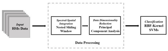
Figure 1.
Structure of the proposed Nested Sliding Window (NSW)–Principal Component Analysis (PCA)–Support Vector Machine (SVM) model.
The original hyperspectral data is a three-dimensional cube, which can be expressed as , where represents the set of real numbers and represents that the image has three dimensions, including two spatial dimensions (i.e., H and W) and one spectral dimension (i.e., B). For , there are a total of pixels, and each pixel is a B-dimensional vector. In fact, not all pixels in HSIs have a category label, and only pixels with labels will be used as target pixels for reconstruction. Therefore, the data reconstructed by NSW is transformed into a two-dimensional matrix, i.e., , where N represents the number of pixels with labels. Dimensionality reduction using PCA maps to , where C represents the number of principal components, and . According to the sample size of the training set specified in Section 3, a specified number of samples are randomly selected from as the training set, and the remaining samples are all as the test set, in which the training set is used to train SVM.
2.1. The Nested Sliding Window Method
Due to the continuity of the hyperspectral imaging area, it can theoretically be considered that adjacent pixels have the same category label. However, at the junction of the areas where two different ground targets are located, adjacent pixels obviously do not share the same label. The nested sliding window (NSW) method proposed in this paper uses the correlation between HSI pixels to reconstruct the data, and generally uses the Pearson correlation coefficient to measure the correlation. For pixel vectors and , the Pearson correlation coefficient is calculated as follows:
where represents covariance, and represents variance.
Denote the pixel vector in row i and column j of as , and assume that is the target pixel. define a neighborhood with a size of that contains the surrounding pixels of :
where , , .
Considering that Formula (2) cannot be used to obtain the neighborhood when the target pixel is at the edge position of in the spatial dimension, i.e., , , , or , the data needs to be zero-padding before obtain the neighborhood. Perform zero-padding operation on to get :
After zero-padding is performed on the raw data, the neighborhood of the target pixel can be obtained according to Formula (2), denoted as . Set a sliding sub-window with a size of in the neighborhood. Using this sub-window, a smaller three-dimensional matrix can be divided in , where , m and n are used to determine the position of the sliding window, and , . is defined as follows:
where and .
Within the valid range of m and n, always contains the target pixel . Therefore, the correlation coefficients between and the pixel vectors in can be calculated according to Formula (1), and the calculated correlation coefficient matrix be denoted as :
Let the mean value of the elements in the matrix be . When the position of the sliding sub-window changes, i.e., when the values of m and n change, will change accordingly. Assuming , then the and corresponding to can be obtained according to Formulas (4) and (5), respectively, which would be used to reconstruct the target pixel. First, change the shape of from to , and change the shape of from to . Second, expand the reshaped from a one-dimensional vector to a two-dimensional matrix, denoted as :
The formula for reconstruction of is as follows:
where is the reconstructed pixel of the current target pixel, which is a one-dimensional vector; represents the element-wise product (i.e., the Hadamard product) of and ; represents the sum of the elements in a vector (or matrix).
Every time m and n change, a calculation of is performed, which actually causes a lot of repeated calculations. Therefore, it is better to calculate the correlation coefficient of and the pixels in the neighborhood at the beginning. The resulting correlation coefficient matrix is as follows:
where represents the correlation coefficient between and . Therefore, can be obtained directly by partition in .
In fact, only a fraction of the pixels in the dataset used for the experiment have category labels. If all the pixels in the dataset are reconstructed, there will be a lot of useless computational overhead. Therefore, a pixel needs to be reconstructed based on whether it has a category label. For the three-dimensional hyperspectral dataset , there is a corresponding label matrix , and the elements in correspond to the pixel vectors in . Generally, pixels without a category label are uniformly assigned a 0-label to facilitate culling during analysis. For this reason, in the NSW method, pixels with a label of 0 will be skipped without processing; pixels with a label of non-zero will be used as the target pixels for reconstruction.
The pseudo code of NSW is shown in Algorithm 1.
| Algorithm 1 Nested Sliding Window algorithm. |
|
An example is given to graphically illustrate the general processing flow of the NSW method, as shown in Figure 2.
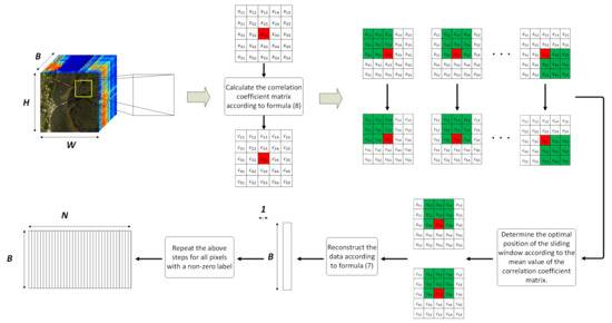
Figure 2.
An example of the general flow of the NSW method.
In the example given in Figure 2, the size of the neighborhood is . By calculating the correlation coefficients between the target pixel and all pixels in the neighborhood, a correlation coefficient matrix of size is obtained. Whenever the position of the sliding sub-window changes, a subset of pixels with a size of is partitioned from the neighborhood, and a corresponding subset of correlation coefficients with a size of is obtained, too. The pixel subset contains 1 target pixel (marked in red) and 8 adjacent pixels (marked in green). By comparing the mean values of different correlation coefficient matrix subsets, the maximum one corresponds to the optimal position of the sliding sub-window. Assuming that the correlation coefficient matrix subset corresponding to the optimal sub-window in Figure 2 is , and the corresponding pixel subset is . When performing reconstruction, first expand from a one-dimensional vector to a two-dimensional matrix (donated as ). In the expanded matrix, the value of each row is the same, that is, all are . The reconstruction is carried out according to Formula (7), namely:
2.2. Dimensionality Reduction and Classifier
In the proposed NSW-PCA-SVM model, PCA [51] is used for dimensionality reduction of the data reconstructed by NSW, and RBF-kernel SVM [51] is used for classification. In Section 2.2, PCA and RBF-kernel SVM are introduced in two subsections, respectively.
2.2.1. Principal Component Analysis
Principal component analysis (PCA) is one of the most commonly used dimensionality reduction algorithms. It learns the low-dimensional representation of data to achieve the purpose of dimensionality reduction and denoising.
After the reconstruction of the original data using NSW method, a two-dimensional matrix with B rows and N columns is obtained, denoted as R. The matrix contains n samples, and each sample is a B-dimensional vector. Before using PCA for dimensionality reduction, it is necessary to centralize the reconstructed data, that is, , where represents a sample in the reconstructed dataset.
Assuming that the reconstructed data needs to be reduced from B-dimension to d-dimension, the purpose of PCA is to find a two-dimensional transformation matrix with B rows and d columns, denoted as W. The variance of the projected sample points is expected to be maximized, where the projection of the sample point is . Therefore, the variance of the projected sample is , and the optimization goal is as follows:
where represents the trace of the matrix, and each column vector (denoted as ) in W is an standard orthonormal basis vector, which means, , and .
Using Lagrange Multiplier Method for Equation (10), , where represents the eigenvalue of the covariance matrix . Assuming that the eigenvalues are sorted: , then , and the dimensionality reduction data is .
2.2.2. RBF-Kernel Support Vector Machine
Support Vector Machine (SVM) is one of the most influential algorithms in supervised classifiers, which is used to solve binary-classification tasks. By combining multiple binary-class SVMs, a multi-class classifier can be obtained. A common combination strategy is One-Versus-One (OVO), which implements multi-classification by designing SVMs between every two categories. Assuming classification for a dataset with k categories, the number of binary-class SVMs that OVO-SVMs need to design is . Considering the classification results of all the binary-class SVMs, the predicted value with the highest frequency is the final classification result.
For a given training set , where , the binary-class SVM needs to find a hyperplane (i.e., ) to make the best segmentation of the sample points. Assuming that the hyperplane correctly classifies the training samples, for , there is
Let
the sum of the distances from the two heterogeneous support vectors to the hyperplane is
where the support vector refers to the sample point closest to the hyperplane that makes Formula (12) true. The distance in Formula (13) is also called margin. Therefore, the goal of SVM is to find the partitioning hyperplane with the maximum margin, that is, to find the w and b that maximize and satisfy the constraints in Formula (12). Since maximizing only needs to maximize , which is equivalent to minimizing , that is, satisfying
This equivalent transformation makes solving Formula (14) a convex optimization problem.
Obviously, SVM solves the classification problem in a linear manner. For linearly inseparable data, the training sample can be linearly separable in the transformed eigenspace by introducing a kernel function. The Gaussian Kernel Function (also known as Radial Basis Function, RBF) is one of the commonly used kernel functions:
where is the bandwidth of the Gaussian kernel (width).
3. Datasets and Model Validation
3.1. Datasets
In order to verify the validity of the proposed model, three publicly available hyperspectral remote sensing datasets were selected for experimental testing. These datasets have different scales, spatial resolutions, and spectral resolutions, and are obtained by different hyperspectral sensors. The robustness of the model can be examined by selecting such three datasets for the validation experiment, and these datasets are also commonly used in relevant studies. Among these three datasets, the Indian Pines dataset is available from the Purdue University Research Repository [52], while the Salinas and PaviaU datasets are available from the Computational Intelligence Group from the University of the Basque Country (http://www.ehu.eus/ccwintco/index.php?Title=Hyperspectral_Remote_Sensing_Scenes). In the three Section 3.1.1, Section 3.1.2, Section 3.1.3, we will introduce these datasets in turn, mainly referring to the content provided by the Computational Intelligence Group. We will also introduce the selection rules of training samples for each dataset.
3.1.1. Indian Pines Dataset
The Indian Pines dataset was collected by the AVIRIS sensor at the test site in northwestern Indiana, USA. The dataset contains pixels with a spatial resolution of 20 m/pixel. Since the dataset was collected by an AVIRIS sensor, it has 224 bands of 10 nm width with central wavelengths from 400 to 2500 nm. The original dataset contains 224 bands, which are reduced to 200 bands after excluding 24 water-absorbing bands: (104–108, 150–163, and 220). In the Indian Pines dataset, there are a total of 10,249 pixels with non-zero labels, which belong to 16 categories.
Table 1 shows the number of samples in each category in the Indian Pines dataset, as well as the division of training set and test set. It can be seen that the number of samples in different categories in the Indian Pines dataset is quite different. Some categories, such as Corn-notill, Soybean-mintill, and Woods, etc., have a large number of samples, while some categories, such as Alfalfa, Grass-pasture-mowed, and Oats, etc., have a relatively small number of samples. The uneven distribution of samples brings greater challenges to the classification task. In order to examine the performance of the models more comprehensively, it is necessary to use such data for detection. In the Indian Pines dataset, 20 samples of categories with a sample number greater than 40 are randomly selected to be added into the training set; for categories with a sample number less than 40, half of them are taken to be added into the training set, and the rest samples are all used to form the test set.

Table 1.
The number of samples in each category in the Indian Pines dataset.
3.1.2. Salinas Dataset
The Salinas dataset is also collected by the AVIRIS sensor as the Indian Pines dataset, and the imaged scene is the Salinas Valley in California, USA. Therefore, the Salinas dataset also contains 224 bands of 10 nm width with central wavelengths from 400 to 2500 nm, and it has 204 bands remaining after excluding 20 water absorption bands: (108–112, 154–167, and 224). The dataset contains pixels with a spatial resolution of 3.7 m/pixel. In the Salinas dataset, there are a total of 54,129 pixels with non-zero labels, which belong to 16 categories.
Table 2 shows the number of samples in each category in the Salinas dataset, as well as the division of training set and test set. Although the Salinas dataset also has some categories with a large number of samples and some categories with a relatively few samples, all categories can select 20 samples to form the training set. Therefore, the uneven sample distribution of the Salinas dataset does not actually have much impact on the classification effect of the model.
Table 2.
The number of samples in each category in the Salinas dataset.
3.1.3. PaviaU Dataset
The PaviaU dataset was collected by the ROSIS sensor over several areas of the University of Pavia. The dataset contains pixels, and its spatial resolution is 1.3 m/pixel, which is the highest among the three datasets used for testing in this paper. There is a large contiguous area in this dataset that does not contain usable information, so the actual available dataset only contains pixels. The PaviaU dataset contains 103 bands of 6 nm width with central wavelengths from 430 to 860 nm. In this dataset, there are a total of 54,129 pixels with non-zero labels, which belong to 16 categories.
Table 3 shows the number of samples in each category in the PaviaU dataset, as well as the division of training set and test set. In the PaviaU dataset, 20 samples of each category were randomly selected to form the training set, and the remaining samples formed the test set.
Table 3.
The number of samples in each category in the PaviaU dataset.
3.2. Model Validation
Since the proposed model can be regarded as an improvement based on the pixel-wise SVM classification model, the simple RBF-kernel SVM was used for comparison. Since the addition of PCA in NSW-PCA-SVM is one of the important factors that affect the final classification effect, the PCA-SVM model was also used for comparison. In order to verify the necessity of PCA, the NSW-SVM model without PCA was also used for comparison. In addition, six state-of-the-art models were selected for comparative analysis, i.e., CDCT-WF-SVM [28], CDCT-2DCT-SVM [28], SDWT-2DWT-SVM [53], SDWT-WF-SVM [53], SDWT-2DCT-SVM [53] and Two-Stage [54]. The six advanced models used for comparison come from three published papers. In these papers, the datasets used in the experiment are the same as those used in our paper. The difference is that these papers use far more samples for model training than our paper does. Among these six models, the first five models belong to the “pre-processing before classification” model, and the sixth model belongs to the “processing after classification” model.
(1) CDCT-WF-SVM: This model uses a one-dimensional Discrete Cosine Transform (1D-DCT) to obtain the spectral profile representation of the HSI, and for the high-frequency components of the representation, a two-dimensional adaptive Wiener filter (2D-AWF) is used to extract spatial information. After combining the low-frequency components with the processed high-frequency components, a one-dimensional inverse DCT is used for transformation to obtain the final pre-processed data. Finally, SVM is used for classification.
(2) CDCT-2DCT-SVM: The structure of this model is similar to CDCT-WF-SVM, except that the 2D-AWF is replaced with a 2D-DCT.
(3) SDWT-2DWT-SVM: This model uses Discrete Wavelet Transform (DWT) to decompose HSI in multiple stages in the spectral dimension, and uses 2D-DWT to extract spatial information for each stage. Then, Perform DWT reconstruction on the combined data to obtain the final pre-processed data. Finally, SVM is used for classification.
(4) SDWT-WF-SVM: The structure of this model is similar to SDWT-2DWT-SVM, except that the 2D-DWT is replaced with a 2D-WF.
(5) SDWT-2DCT-SVM: The structure of this model is similar to SDWT-2DWT-SVM, except that the 2D-DWT is replaced with a 2D-DCT.
(6) Two-Stage: This model contains two processing stages. The first stage is to use SVM to obtain a pixel-wise classification probability map, and the second stage is to use a variational denoising method to reconstruct the classification map.
The three evaluation indicators used in this paper to measure the classification performance of the models are Overall Accuracy (OA), Average Accuracy (AA) and Kappa coefficient () [55]. OA reflects the proportion of correctly classified samples in the test sample. AA is obtained by calculating the classification accuracy of each category and taking the arithmetic average. When there is a large gap in the number of different samples in the dataset, the OA of the classification is easily affected by the category with a large sample size. Therefore, it is difficult to reflect the real level of the model performance using only OA. Kappa coefficient can reflect the comprehensive performance of classification model on OA and AA.
In the experimental verification, this paper repeated all the experiments for 10 times and took the average values as the final experimental results to reduce the influence of random factors. Three evaluation indicators (i.e., OA, AA and ) can be calculated by the confusion matrix [56], whose form is as
where represents the number of samples whose real label is the i-th class and is classified as the j-th class, .
The formula for calculating OA according to the confusion matrix is as follows:
The formula for calculating AA according to the confusion matrix is as follows:
The formula for calculating according to the confusion matrix is as follows:
Therefore, the average OA, AA and can be calculated according to Formulas (17),(18),(19) by calculating the mean value of the confounding matrices obtained from 20 experiments.
The experiments were performed on a computer with an Intel Core i7-8750H CPU, 8 GB RAM, and all the methods were implemented with Python 3.
4. Experimental Results and Analysis
In this section, the classification performance of the proposed model was tested and analyzed experimentally on three public datasets. Firstly, the values of the two main parameters in the NSW-PCA-SVM model (i.e., neighbor size and principal component number) were measured. Secondly, the best classification results of NSW-PCA-SVM on three datasets are given, and compared with the best results of two basic pixel-wise classification models and six state-of-the-art models based on filtering. Finally, the classification results of NSW-PCA-SVM and various comparison models under different training set sample sizes are presented.
4.1. Model Validation
There are two key parameters, namely neighborhood size and principal component number, which have a significant impact on the performance of the NSW-PCA-SVM model. The value of the neighborhood size (denoted as ) determines the value of a in Formula (2), i.e., . According to the description of the NSW algorithm in Section 2.1, the value of directly affects the number of related pixels during reconstruction. When the value of is large, the reconstructed pixels are more affected by the related pixels. Conversely, when the value of is small, the reconstructed pixels are less affected by the related pixels.
Since each dataset has a different spatial resolution, it is necessary to conduct different experiments for different datasets when determining the value of , where the value range of is . For the NSW-SVM model, the OAs corresponding to different values of were obtained, and the optimal value of corresponded to the largest OA. Since the result of NSW-PCA-SVM is determined by two parameters, when determining the optimal value of , it is necessary to consider the optimal values of the principal component number corresponding to different .
Figure 3 shows the OAs of NSW-SVM and NSW-PCA-SVM corresponding to different values of on the Indian Pines, Salinas and PaviaU datasets. As shown in Figure 3a, on the Indian Pines dataset, when , both NSW-SVM and NSW-PCA-SVM achieved the highest OA. As shown in Figure 3b, on the Salinas dataset, the highest OA of NSW-SVM was obtained when , and the highest OA of NSW-PCA-SVM was obtained when . As shown in Figure 3c, on the PaviaU dataset, the highest OA of NSW-SVM was obtained when , and the highest OA of NSW-PCA-SVM was obtained when .
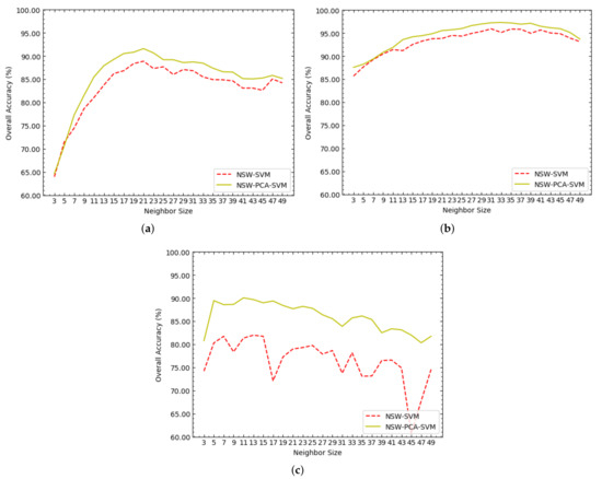
Figure 3.
The overall accuracies (OAs) of NSW-SVM and NSW-PCA-SVM corresponding to different values of on the three datasets, where (a–c) represent the experimental results in Indian Pines, Salinas and PaviaU datasets, respectively.
According to the trend of each curve in Figure 3, the following three conclusions can be drawn:
(1) All the curves basically showed a trend of increasing first and then decreasing, which is particularly obvious in Figure 3a,b. In the NSW method, the value of determines the number of related pixels in the neighborhood. When the value of is larger, the neighborhood contains relatively more related pixels, including homogeneous pixels and heterogeneous pixels. Therefore, although a larger value of makes the reconstructed pixels contain richer useful information, which is provided by homogeneous pixels, it also makes the reconstructed pixels contain more interference information, which is provided by heterogeneous pixels. On the contrary, a smaller value of makes the reconstructed pixels contain less interference information, but at the same time it makes the reconstructed pixels contain less useful information. Therefore, whether the value of is too large or too small will cause the classification accuracy of the NSW-PCA-SVM model to decrease.
(2) When the dataset is unchanged, the optimal values of in NSW-SVM and NSW-PCA-SVM are close. Therefore, the optimal value of in NSW-PCA-SVM can be roughly determined according to the optimal value of in NSW-SVM, so as to reduce the experimental testing required for parameter adjustment.
(3) When NSW-SVM and NSW-PCA-SVM achieved the best classification effect, the values of on the Salinas dataset were both greater than those on the Indian Pines dataset. The reason is that the spatial resolution of the Salinas dataset is larger than that of the Indians Pines dataset. When other conditions are the same or similar, the larger the spatial resolution of HSI is, the more homogeneous pixels that can be contained in the neighborhood.
For any non-adaptive dimensionality reduction algorithm, the dimension of the data after dimensionality reduction needs to be determined in advance. The principal component number of PCA is the dimension of the dataset after dimensionality reduction, denoted as c. When performing experimental determination on the value of c, it is also necessary to consider the optimal value of corresponding to different values of c.
It can be seen from Figure 4 that the three curves generally show a trend of first increasing and then decreasing. Therefore, the possible range of the optimal value of c can be investigated in a sparse value interval, such as . According to Figure 4, the optimal value of c in NSW-PCA-SVM on the three datasets can be determined: on the Indian Pines dataset, ; on the Salinas dataset, ; on the PaviaU dataset, .
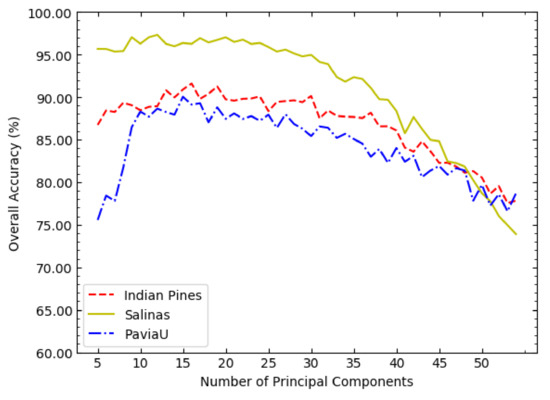
Figure 4.
The OAs of NSW-PCA-SVM corresponding to different values of c on the three datasets.
According to the experimental results, the parameter settings of NSW-SVM and NSW-PCA-SVM on the three datasets are obtained, as shown in Table 4.
Table 4.
Parameter settings of NSW-SVM and NSW-PCA-SVM on three datasets.
The experimental results of the five state-of-the-art comparison models are obtained according to the codes provided by the authors of the original papers, so the parameters of each comparison model are set according to the original papers. For the basic SVM model and PCA-SVM model, the best parameters were determined based on experiments.
SVM: The kernel function is RBF, the kernel coefficient is 0.125, and the regularization parameter is 200. The above parameter settings are applicable to the experiments on the three datasets, and are applicable to the SVM part of all models in this paper.
PCA-SVM: The principal component number of PCA is 6 on the Indian Pines dat aset, 4 on the Salinas dataset, and 11 on the PaviaU dataset.
4.2. Classification Results on the Indian Pines Dataset
In Section 4.2, the classification performances of NSW-SVM and NSW-PCA-SVM were tested on the Indian Pines dataset. Table 5 shows the specific classification results of each model, including the classification accuracy of each class, overall classification accuracy (OA), average classification accuracy (AA) and Kappa coefficient (), where the sample size of the training set is shown in Table 1.
Table 5.
Specific classification results of each model on the Indian Pines dataset, where Model-1, Model-2, ..., Model-10 represents SVM, PCA-SVM, CDCT-WF-SVM, CDCT-2DCT-SVM, SDWT-2DWT-SVM, SDWT-WF-SVM, SDWT-2DCT-SVM, Two-Stage, NSW-SVM and NSW-PCA-SVM, respectively, and the same in the other figures and tables.
According to Table 5, on the Indian Pines dataset, NSW-PCA-SVM achieved the best classification result (). The Kappa coefficient in the classification results of each model is mainly determined by OA, which is the reason why NSW-PCA-SVM () achieved a high Kappa value. However, the classification result of the proposed model performed worse on AA than the six state-of-the-art comparison models. By analyzing the classification results of various classes of samples, it can be seen that NSW-PCA-SVM achieved low classification accuracy in the classification of samples of category 1, 7 and 9. According to Table 1, the Indian Pines dataset has a small number of samples in categories 1, 7 and 9, which makes it difficult for NSW method to obtain effective spatial information and results in poor final classification results.
By comparing the classification results with the basic SVM model and the PCA-SVM model, it can be seen that 8 models utilizing the spatial information of HSIs were significantly improve the classification accuracy. Figure 5 shows the classification maps of each model on the Indian Pines dataset. According to Figure 5, the classification maps of the two pixel-based classification models (SVM and PCA-SVM) contained a large amount of classification noise, while the classification maps of the models utilizing the spatial information contained much less classification noise. In addition, by observing the classification maps of NSW-SVM and NSW-PCA-SVM, it can be seen that the classification maps of the two models contained less noise for the categories with more samples. On the contrary, they contain more noise for the categories with less samples.
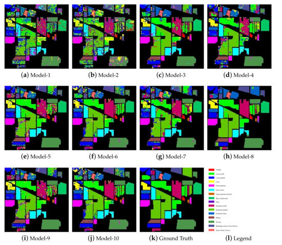
Figure 5.
Classification maps of the models on the Indian Pines dataset.
In order to investigate the impact of the size of the training set on the classification accuracy of the models, this paper tested the OAs of each model under different sizes of the training set, as shown in Figure 6. According to Figure 6, with the increase of the sample size of the training set, the increase amplitudes of the OAs of NSW-SVM and NSW-PCA-SVM were smaller than that of other comparison models. With the increase of the sample size of the training set, the OAs of the six state-of-the-art classification models were getting closer to NSW-PCA-SVM. In particular, when the number of samples in the training set exceeds 60 samples/class, the overall classification accuracy of NSW-PCA-SVM is worse than that of the Two-Stage model. Figure 6 can show the advantage of NSW-PCA-SVM under a small sample size of the training set.
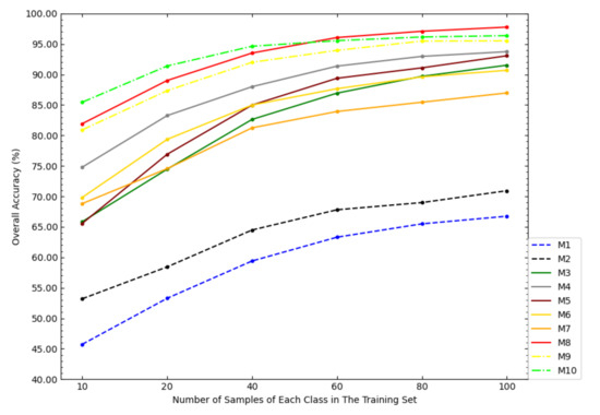
Figure 6.
The OAs of each model in the Indian Pines dataset under the partitioning of training sets of different sizes.
4.3. Classification Results on the Salinas Dataset
In Section 4.3, the classification performances of NSW-SVM and NSW-PCA-SVM were tested on the Salinas dataset. Table 6 shows the specific classification results of each model, including classification accuracy of each category, overall classification accuracy (OA), average classification accuracy (AA) and Kappa coefficient (), where the sample size of the training set is shown in Table 2.
Table 6.
Specific classification results of each model on the Salinas dataset.
According to Table 6, on the Salinas dataset, NSW-PCA-SVM achieved the best classification result (), while NSW-SVM achieved the sub-optimal result (). Different from the Indian Pines dataset, the AAs of the two proposed models on the Salinas dataset were better than that of the comparison models, except for the Two-Stage model. According to Table 2, although the number of samples in each category of the Salinas dataset were not similar, there is no case where the number of samples in several categories were particularly small.
Figure 7 shows the classification maps of each model on the Salinas dataset. According to Figure 6, the classification noises contained in the classification maps of NSW-SVM and NSW-PCA-SVM were far less than other classification models, especially the two basic models. According to Figure 7k, it can be seen that the distribution of similar samples was very concentrated, which enables the NSW method to effectively extract the spatial information of the Salinas dataset to improve the classification effect.
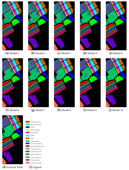
Figure 7.
Classification maps of the models on the Salinas dataset.
Figure 8 shows the OAs of each model on the Salinas dataset under different sample sizes of the training set. According to Figure 8, when the sample size of the training set was small, the OA of NSW-PCA-SVM was much higher than that of the comparison models. However, as the sample size of the training set increased, the advantage of the proposed model over the comparison models was gradually weakening, especially when the sample size of the training set is 100 samples/class, the OA of SDWT-2DCT-SVM was very close to NSW-PCA-SVM and the OA of Two-Stage was higher than NSW-PCA-SVM. Figure 8 also reflected the superiority of NSW-PCA-SVM under a small sample size of the training set.
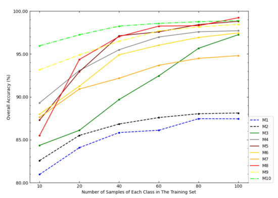
Figure 8.
The OAs of each model in the Salinas dataset under the partitioning of training sets of different sizes.
4.4. Classification Results on the PaviaU Dataset
In Section 4.4, the classification performances of NSW-SVM and NSW-PCA-SVM were tested on the PaviaU dataset. Table 7 shows the specific classification results of each model, including the classification accuracy of each category, overall classification accuracy (OA), average classification accuracy (AA) and Kappa coefficient (), where the sample size of the training set is shown in Table 3.
Table 7.
Specific classification results of each model on the PaviaU dataset.
According to Table 7, on the PaviaU dataset, NSW-PCA-SVM also achieved the best classification results (). In addition, although NSW-PCA-SVM achieved the best OA, it was slightly lower than Two-Stage on AA. Figure 9 shows the classification maps of each model on the PaviaU dataset. According to Figure 9, the classification map of NSW-PCA-SVM contained less noise, which corresponds to the classification results in Table 7. According to Figure 9k, it can be seen that except for a few categories, the sample distribution of the same categories was scattered. Therefore, it difficult for the NSW method to effectively extract the spatial information of the PaviaU dataset.
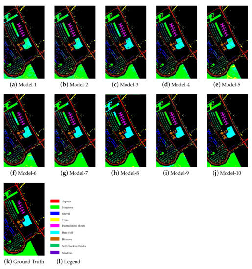
Figure 9.
Classification maps of the models on the PaviaU dataset.
Figure 10 shows OAs of each model on the PaviaU dataset under different sample sizes of the training set. It can be seen from Figure 10 that the classification effect of NSW-PCA-SVM compared to the six state-of-the-art models achieveed greater advantages when the sample size of the training set was small. However, as the sample size of the training set increased, the advantage was gradually weakening. The result was similar to the those on the first two datasets. For example, when the sample size of the training set exceeds 60 samples/class, the OA of the Two-Stage model exceeded that of NSW-PCA-SVM.

Figure 10.
The OAs of each model in the PaviaU dataset under the partitioning of training sets of different sizes.
Table 8 shows the running time of the proposed NSW-SVM, NSW-PCA-SVM and the eight models used for comparison. It can be seen that the running time of the original SVM model or the PCA-SVM model is very short. The reason is that the SVM algorithm and PCA algorithm called in the program are actually developed based on the C Programming Language. Compared with the comparison models, the two models based on NSW require more computational time. The main computational cost lies in the calculation of correlation coefficient matrices according to formula (6). In fact, after the neighbourhoods are divided using formula (2), the reconstruction of each target pixel is independent of each other. Therefore, parallel computing techniques can be used to improve the calculation speed of the NSW algorithm. If the GPU is used for running acceleration, the running time of the NSW algorithm can be greatly reduced.
Table 8.
Running time (seconds) for the classification for Indian Pines, Salinas, PaviaU datasets by various models.
5. Discussion
In the experimental part, we conducted experimental tests on the proposed NSW-PCA-SVM model and the models for comparison on three datasets. The performance of all models on the three datasets is relatively consistent, so the following analysis is based on the experimental results on the Indian Pines dataset. By analysing the experimental results, the following conclusions can be drawn:
(1) The two basic models, SVM and PCA-SVM, only consider the spectral information of the HSI, their classification accuracy is worse than other models that additionally consider spatial information. The classification accuracy of the NSW-SVM model (OA = 87.35%) is much higher than that of the SVM model (OA = 53.29%), and the classification accuracy of the NSW-PCA-SVM model (OA = 91.40%) is also much higher than that of the PCA-SVM model (OA = 58.44%), which shows that the NSW method can effectively extract the spatial information of HSI and significantly improve the classification performance of the models.
(2) The classification accuracy of the five comparison models, i.e., CDCT-WF-SVM, CDCT-2DCT-SVM, SDWT-2DWT-SVM, SDWT-WF-SVM and SDWT-2DCT-SVM, has been significantly improved compared with the SVM model and the PCA-SVM model. Among them, the CDCT-2DCT-SVM model (OA = 83.26%) achieved the highest classification accuracy. In fact, the CDCT-2DCT-SVM model and the other four models only perform spatial filtering on the noisy part from the spectral filter, while a part of the reconstructed data does not contain spatial information. However, the NSW method considers all spectral bands when extracting the spatial information of HSIs. Therefore, the classification results of the NSW-PCA-SVM model (OA = 91.40%, AA = 84.00%, Kappa = 90.20%) were better than those of the CDCT-2DCT-SVM model (OA = 83.26%, AA = 89.48%, Kappa = 81.07%) and the other four models.
(3) In our comparative experiment, we chose a “processing after classification” model, namely Two-Stage. Since the main classification stage of the Two-Stage model is based on pixel-wise classification, when the sample size of the training set is small, the OA of Two-Stage (OA = 89.02%) is lower than that of NSW-PCA-SVM (OA = 91.04%). The Two-Stage model uses a variational denoising method to restore the classification map, which allows the model to ignore the uneven sample distribution, so the AA of Two-Stage (AA = 94.64%) is higher than the NSW-PCA-SVM model (AA = 84.00%). It can also be seen from Figure 5 that the classification map obtained by using the Two-Stage model contains less noise, but there are cases where all pixels in a certain area are classified incorrectly.
(4) When the number of samples in the training set is small, such as 20 samples/class, the advantage of the NSW-PCA-SVM model in OA can reach 2.38–38.11% over the comparison models. According to Figure 6, Figure 8 and Figure 10, further reducing the number of training set samples, such as 10 samples/class, would further expand the advantage of the NSW-PCA-SVM model. On the contrary, as the number of samples in the training set increases, the advantage of the NSW-PCA-SVM model decreases continuously. According to Table 8, the NSW-PCA-SVM model requires more computational time than other models, although it can be further optimized. Therefore, only when the number of samples in the training set is small, such as 10 samples/class, 20 samples /class or 40 samples/class, etc., the use of NSW-PCA-SVM for classification can achieve higher returns.
Another disadvantage of the NSW-PCA-SVM model is that when the distribution of homogeneous samples of the HSI in the spatial dimension is scattered, it is difficult for the NSW method to extract spatial information very effectively. For example, on the PaviaU dataset, the classification accuracy of NSW-PCA-SVM did not have a great advantage. According to Table 7, the advantage of the NSW-PCA-SVM model in OA only achieves 1.61–18.40% over the comparison models.
6. Conclusions
Based on the correlation between pixels, a Nested Sliding Window (NSW) method is proposed to extract the spatial features of HSIs. The NSW method can be used to reconstruct the pixels of HSIs, and the reconstructed pixels contain the information of the original pixels and the pixels that are in a spatially adjacent relationship with them. For the reconstructed data, PCA is used for dimensionality reduction to further eliminate the noise in the spectral dimension. Finally, the RBF-kernel SVM is used to classify the processed data. The NSW-PCA-SVM model has been tested experimentally on three public datasets. By comparing with the SVM model and the PCA-SVM model that only consider the spectral information of HSIs, the proposed model based on the NSW method can significantly improve the classification accuracy. Compared with five filter-based comparison approaches, NSW can extract spatial features for all spectral bands of HSIs. Compared with the “processing after classification” model, i.e., the Two-Stage model, the NSW-PCA-SVM model also has obvious advantages when the training set sample size is small. Therefore, our main contribution is to propose an effective classification model with limited training samples.
The limitations of NSW-PCA-SVM are: when the number of training set samples is large, it is difficult for NSW-PCA-SVM to obtain the advantages in classification accuracy, especially the NSW method requires more computational time; on datasets where homogeneous samples are closely adjacent in spatial relationship, such as Indian Pines and Salinas datasets, NSW-PCA-SVM has greater advantages, while for the datasets with dispersed spatial relations of homogeneous samples, such as PaviaU dataset, NSW-PCA-SVM are difficult to achieve significant advantages. For the improvement of the NSW method, we will carry out the following goals in future work: consider using more reasonable parameters to measure the degree of correlation between homogeneous samples; consider more reasonable reconstruction methods to avoid heterogeneous pixels participating in reconstruction; consider different neighborhood division methods, including the division with irregular shapes.
Author Contributions
All the authors made significant contributions to the work. J.R., R.W. and W.W. designed the research, analysed the results, and accomplished the validation work. G.L. and Y.W. provided advice for the preparation and revision of the paper. All authors have read and agreed to the published version of the manuscript.
Funding
The work described in this paper was supported by the National Natural Science Foundation of China (U1711267), Hubei Province Innovation Group Project (2019CFA023), Fundamental Research Funds for the Central Universities, China University of Geosciences (Wuhan) (CUGCJ1810), and the Open Fund of Hubei Key Laboratory of Intelligent Geo-Information Processing (KLIGIP2018 and ZRIGIP-201801).
Institutional Review Board Statement
Not applicable.
Informed Consent Statement
Not applicable.
Data Availability Statement
Publicly available datasets were analyzed in this study. This data can be found here: http://www.ehu.eus/ccwintco/index.php?Title=Hyperspectral_Remote_Sensing_Scenes.
Acknowledgments
We wish to thank the authors of the papers [28,53,54] for providing us with their experimental source code, which facilitates our comparison with their models in our experiments.
Conflicts of Interest
The authors declare no conflict of interest. The founding sponsors had no role in the design of the study; in the collection, analyses, or interpretation of data; in the writing of the manuscript; and in the decision to publish the results.
References
- Wang, C.L.; Ren, J.; Wang, H.W.; Zhang, Y.; Wen, J. Spectral–spatial classification of hyperspectral data using spectral-domain local binary patterns. Multimed. Tools Appl. 2018, 77, 29889–29903. [Google Scholar] [CrossRef]
- Tiwari, K.C.; Arora, M.K.; Singh, D. An assessment of independent component analysis for detection of military targets from hyperspectral images. Int. J. Appl. Earth Obs. Geoinf. 2011, 13, 730–740. [Google Scholar] [CrossRef]
- Heiden, U.; Heldens, W.; Roessner, S.; Segl, K.; Esch, T.; Mueller, A. Urban structure type characterization using hyperspectral remote sensing and height information. Landsc. Urban Plan. 2012, 105, 361–375. [Google Scholar] [CrossRef]
- Im, J.; Jensen, J.R.; Jensen, R.R.; Gladden, J.; Waugh, J.; Serrato, M. Vegetation cover analysis of hazardous waste sites in Utah and Arizona using hyperspectral remote sensing. Remote Sens. 2012, 4, 327–353. [Google Scholar] [CrossRef]
- Akbari, H.; Kosugi, Y.; Kojima, K.; Tanaka, N. Detection and analysis of the intestinal ischemia using visible and invisible hyperspectral imaging. IEEE Trans. Biomed. Eng. 2010, 57, 2011–2017. [Google Scholar] [CrossRef]
- Wahabzada, M.; Mahlein, A.K.; Bauckhage, C.; Steiner, U.; Oerke, E.C.; Kersting, K. Plant phenotyping using probabilistic topic models: Uncovering the hyperspectral language of plants. Sci. Rep. 2016, 6, 1–11. [Google Scholar] [CrossRef]
- Melgani, F.; Bruzzone, L. Classification of hyperspectral remote sensing images with support vector machines. IEEE Trans. Geosci. Remote Sens. 2004, 42, 1778–1790. [Google Scholar] [CrossRef]
- Bandos, T.V.; Bruzzone, L.; Camps-Valls, G. Classification of hyperspectral images with regularized linear discriminant analysis. IEEE Trans. Geosci. Remote Sens. 2009, 47, 862–873. [Google Scholar] [CrossRef]
- Belgiu, M.; Drăguţ, L. Random forest in remote sensing: A review of applications and future directions. ISPRS J. Photogramm. Remote Sens. 2016, 114, 24–31. [Google Scholar] [CrossRef]
- Ma, L.; Crawford, M.M.; Tian, J. Local manifold learning-based k-nearest-neighbor for hyperspectral image classification. IEEE Trans. Geosci. Remote Sens. 2010, 48, 4099–4109. [Google Scholar] [CrossRef]
- Shahdoosti, H.R.; Mirzapour, F. Spectral–spatial feature extraction using orthogonal linear discriminant analysis for classification of hyperspectral data. Eur. J. Remote. Sens. 2017, 50, 111–124. [Google Scholar] [CrossRef]
- Mei, S.; Ji, J.; Hou, J.; Li, X.; Du, Q. Learning sensor-specific spatial–spectral features of hyperspectral images via convolutional neural networks. IEEE Trans. Geosci. Remote Sens. 2017, 55, 4520–4533. [Google Scholar] [CrossRef]
- Zhang, M.; Li, W.; Du, Q. Diverse region-based CNN for hyperspectral image classification. IEEE Trans. Image Process. 2018, 27, 2623–2634. [Google Scholar] [CrossRef]
- Zhao, C.; Liu, W.; Xu, Y.; Wen, J. A spectral–spatial SVM-based multi-layer learning algorithm for hyperspectral image classification. Remote Sens. Lett. 2018, 9, 218–227. [Google Scholar] [CrossRef]
- Dópido, I.; Li, J.; Marpu, P.R.; Plaza, A.; Dias, J.M.B.; Benediktsson, J.A. Semisupervised self-learning for hyperspectral image classification. IEEE Trans. Geosci. Remote Sens. 2013, 51, 4032–4044. [Google Scholar] [CrossRef]
- Wang, Y.; Duan, H. Classification of hyperspectral images by SVM using a composite kernel by employing spectral, spatial and hierarchical structure information. Remote Sens. 2018, 10, 441. [Google Scholar] [CrossRef]
- Liao, J.; Wang, L.; Zhao, G.; Hao, S. Hyperspectral image classification based on bilateral filter with linear spatial correlation information. Int. J. Remote Sens. 2019, 40, 6861–6883. [Google Scholar] [CrossRef]
- Benediktsson, J.A.; Palmason, J.A.; Sveinsson, J.R. Classification of hyperspectral data from urban areas based on extended morphological profiles. IEEE Trans. Geosci. Remote Sens. 2005, 43, 480–491. [Google Scholar] [CrossRef]
- Liao, W.; Bellens, R.; Pizurica, A.; Philips, W.; Pi, Y. Classification of hyperspectral data over urban areas using directional morphological profiles and semi-supervised feature extraction. IEEE J. Sel. Top. Appl. Earth Obs. Remote Sens. 2012, 5, 1177–1190. [Google Scholar] [CrossRef]
- Hou, B.; Huang, T.; Jiao, L. Spectral–spatial classification of hyperspectral data using 3-D morphological profile. IEEE Geosci. Remote Sens. Lett. 2015, 12, 2364–2368. [Google Scholar]
- Imani, M.; Ghassemian, H. Edge patch image-based morphological profiles for classification of multispectral and hyperspectral data. IET Image Process. 2016, 11, 164–172. [Google Scholar] [CrossRef]
- Kumar, B.; Dikshit, O. Hyperspectral image classification based on morphological profiles and decision fusion. Int. J. Remote Sens. 2017, 38, 5830–5854. [Google Scholar] [CrossRef]
- Kumara, B.; Dikshitb, O. Parallel Implementation of Morphological Profile Based Spectral–Spatial Classification Scheme for Hyperspectral Imagery. Int. Arch. Photogramm. Remote Sens. Spat. Inf. Sci. 2016, 7. [Google Scholar] [CrossRef]
- Wu, K.; Jia, S. 2D Gabor-Based Sparse Representation Classification for Hyperspectral Imagery. In Proceedings of the 2018 Digital Image Computing: Techniques and Applications (DICTA), Canberra, Australia, 10–13 December 2018; pp. 1–8. [Google Scholar]
- Jia, S.; Xie, H.; Deng, X. Extended morphological profile-based Gabor wavelets for hyperspectral image classification. In Proceedings of the 2018 24th International Conference on Pattern Recognition, Beijing, China, 20–24 August 2018; pp. 782–787. [Google Scholar]
- Chen, Y.; Zhu, L.; Ghamisi, P.; Jia, X.; Li, G.; Tang, L. Hyperspectral images classification with Gabor filtering and convolutional neural network. IEEE Geosci. Remote Sens. Lett. 2017, 14, 2355–2359. [Google Scholar] [CrossRef]
- Hanbay, K. Hyperspectral image classification using convolutional neural network and two-dimensional complex Gabor transform. J. Fac. Eng. Archit. Gazi Univ. 2020, 35, 443–456. [Google Scholar]
- Bazine, R.; Wu, H.; Boukhechba, K. Spatial Filtering in DCT Domain-Based Frameworks for Hyperspectral Imagery Classification. Remote Sens. 2019, 11, 1405. [Google Scholar] [CrossRef]
- Liu, X.; Bourennane, S.; Fossati, C. Nonwhite noise reduction in hyperspectral images. IEEE Geosci. Remote Sens. Lett. 2011, 9, 368–372. [Google Scholar] [CrossRef]
- Liu, X.; Feng, Y.; Li, Y.; Liu, X.; Zhao, W.; Fu, M. Denoising hyperspectral images with non-white noise based on tensor decomposition. In Proceedings of the 2016 IEEE International Conference on Digital Signal Processing, Beijing, China, 16–18 October 2016; pp. 437–441. [Google Scholar]
- Nair, P.; Chaudhury, K.N. Fast high-dimensional bilateral and nonlocal means filtering. IEEE Trans. Image Process. 2018, 28, 1470–1481. [Google Scholar] [CrossRef]
- Qian, Y.; Shen, Y.; Ye, M.; Wang, Q. 3-D nonlocal means filter with noise estimation for hyperspectral imagery denoising. In Proceedings of the 2012 IEEE International Geoscience and Remote Sensing Symposium, Munich, Germany, 22–27 July 2012; pp. 1345–1348. [Google Scholar]
- Kang, X.; Xiang, X.; Li, S.; Benediktsson, J.A. PCA-based edge-preserving features for hyperspectral image classification. IEEE Trans. Geosci. Remote Sens. 2017, 55, 7140–7151. [Google Scholar] [CrossRef]
- Tian, W.; Xu, L.; Chen, Z.; Shi, A. Multiple feature learning based on edge-preserving features for hyperspectral image classification. IEEE Access 2019, 7, 106861–106872. [Google Scholar] [CrossRef]
- Tarabalka, Y.; Fauvel, M.; Chanussot, J.; Benediktsson, J.A. SVM-and MRF-based method for accurate classification of hyperspectral images. IEEE Geosci. Remote Sens. Lett. 2010, 7, 736–740. [Google Scholar] [CrossRef]
- Yu, H.; Gao, L.; Li, J.; Li, S.S.; Zhang, B.; Benediktsson, J.A. Spectral–spatial hyperspectral image classification using subspace-based support vector machines and adaptive Markov random fields. Remote Sens. 2016, 8, 355. [Google Scholar] [CrossRef]
- Qing, C.; Ruan, J.; Xu, X.; Ren, J.; Zabalza, J. Spatial–spectral classification of hyperspectral images: A deep learning framework with markov random fields based modelling. IET Image Process. 2018, 13, 235–245. [Google Scholar] [CrossRef]
- Chakravarty, S.; Banerjee, M.; Chandel, S. Spectral–spatial classification of hyperspectral imagery using support vector and fuzzy-MRF. In Proceedings of the International Conference on Intelligent, Secure, and Dependable Systems in Distributed and Cloud Environments, Vancouver, BC, Canada, 25–27 October 2017; pp. 151–161. [Google Scholar]
- Xu, Y.; Wu, Z.; Wei, Z. Markov random field with homogeneous areas priors for hyperspectral image classification. In Proceedings of the 2014 IEEE Geoscience and Remote Sensing Symposium, Quebec City, QC, Canada, 13–18 July 2014; pp. 3426–3429. [Google Scholar]
- Tang, B.; Liu, Z.; Xiao, X.; Nie, M.; Chang, J.; Jiang, W.; Zheng, C. Spectral–spatial hyperspectral classification based on multi-center SAM and MRF. Opt. Rev. 2015, 22, 911–918. [Google Scholar] [CrossRef]
- Cao, X.; Wang, X.; Wang, D.; Zhao, J.; Jiao, L. Spectral–Spatial Hyperspectral Image Classification Using Cascaded Markov Random Fields. IEEE J. Sel. Top. Appl. Earth Obs. Remote Sens. 2019, 12, 4861–4872. [Google Scholar] [CrossRef]
- Wang, Y.; Song, H.; Zhang, Y. Spectral–spatial classification of hyperspectral images using joint bilateral filter and graph cut based model. Remote Sens. 2016, 8, 748. [Google Scholar] [CrossRef]
- Yu, H.; Gao, L.; Li, J.; Zhang, B. Spectral–spatial classification based on subspace support vector machine and Markov random field. In Proceedings of the 2016 IEEE International Geoscience and Remote Sensing Symposium, Beijing, China, 10–15 July 2016; pp. 2783–2786. [Google Scholar]
- Liao, W.; Bellens, R.; Pižurica, A.; Philips, W.; Pi, Y. Classification of hyperspectral data over urban areas based on extended morphological profile with partial reconstruction. In Proceedings of the International Conference on Advanced Concepts for Intelligent Vision Systems, Brno, Czech Republic, 4–7 September 2012; pp. 278–289. [Google Scholar]
- Cao, X.; Xu, Z.; Meng, D. Spectral–spatial hyperspectral image classification via robust low-rank feature extraction and Markov random field. Remote Sens. 2019, 11, 1565. [Google Scholar] [CrossRef]
- Cui, B.; Ma, X.; Zhao, F.; Wu, Y. A novel hyperspectral image classification approach based on multiresolution segmentation with a few labeled samples. Int. J. Adv. Robot. Syst. 2017, 14, 1729881417710219. [Google Scholar] [CrossRef]
- Kang, X.; Li, S.; Benediktsson, J.A. Spectral–spatial hyperspectral image classification with edge-preserving filtering. IEEE Trans. Geosci. Remote Sens. 2013, 52, 2666–2677. [Google Scholar] [CrossRef]
- Cui, B.; Ma, X.; Xie, X.; Ren, G.; Ma, Y. Classification of visible and infrared hyperspectral images based on image segmentation and edge-preserving filtering. Infrared Phys. Technol. 2017, 81, 79–88. [Google Scholar] [CrossRef]
- Jiang, J.; Ma, J.; Chen, C.; Wang, Z.; Cai, Z.; Wang, L. SuperPCA: A superpixelwise PCA approach for unsupervised feature extraction of hyperspectral imagery. IEEE Trans. Geosci. Remote Sens. 2018, 56, 4581–4593. [Google Scholar] [CrossRef]
- Chen, L.; Liu, D.; Huang, S. Decorrelate hyperspectral images using spectral correlation. In Proceedings of the 27th International Congress on High-Speed Photography and Photonics, Xi’an, China, 11 January 2007; Volume 6279, p. 627937. [Google Scholar]
- Goodfellow, I.; Bengio, Y.; Courville, A. Deep Learning; The MIT Press: Cambridge, MA, USA, 2016. [Google Scholar]
- Baumgardner, M.F.; Biehl, L.L.; Landgrebe, D.A. 220 band aviris hyperspectral image dataset: June 12, 1992 indian pine test site 3. Purdue Univ. Res. Repos. 2015, 10, R7RX991C. [Google Scholar]
- Bazine, R.; Wu, H.; Boukhechba, K. Spectral DWT multilevel decomposition with spatial filtering enhancement preprocessingbased approaches for hyperspectral imagery classification. Remote Sens. 2019, 11, 2906. [Google Scholar] [CrossRef]
- Chan, R.H.; Kan, K.K.; Nikolova, M.; Plemmons, R.J. A two-stage method for spectral–spatial classification of hyperspectral images. J. Math. Imaging Vis. 2020, 62, 790–807. [Google Scholar] [CrossRef]
- McHugh, M.L. Interrater reliability: The kappa statistic. Biochem. Medica Biochem. Medica 2012, 22, 276–282. [Google Scholar] [CrossRef]
- Story, M.; Congalton, R.G. Accuracy assessment: A user’s perspective. Photogramm. Eng. Remote Sens. 1986, 52, 397–399. [Google Scholar]


Publisher’s Note: MDPI stays neutral with regard to jurisdictional claims in published maps and institutional affiliations. |
© 2020 by the authors. Licensee MDPI, Basel, Switzerland. This article is an open access article distributed under the terms and conditions of the Creative Commons Attribution (CC BY) license (http://creativecommons.org/licenses/by/4.0/).