Article

Assessment of High Resolution Air Temperature Fields at Rocky Mountain National Park by Combining Scarce Point Measurements with Elevation and Remote Sensing Data

by
Antonio-Juan Collados-Lara
1,2,3,*,
Steven R. Fassnacht
2,3,4,
Eulogio Pardo-Igúzquiza
1 and
David Pulido-Velazquez
1,5
1
Instituto Geológico y Minero de España, Ríos Rosas 23, 28003 Madrid, Spain
2
ESS-Watershed Science, Colorado State University, Fort Collins, CO 80523, USA
3
Natural Resources Ecology Laboratory, Fort Collins, CO 80523, USA
4
Cooperative Institute for Research in the Atmosphere, Fort Collins, CO 80523, USA
5
Campus de los Jerónimos s/n, Universidad Católica de Murcia, Guadalupe, 30107 Murcia, Spain
*
Author to whom correspondence should be addressed.
Remote Sens. 2021, 13(1), 113; https://doi.org/10.3390/rs13010113
Submission received: 18 November 2020 / Revised: 26 December 2020 / Accepted: 28 December 2020 / Published: 31 December 2020

Abstract

:
There is necessity of considering air temperature to simulate the hydrology and management within water resources systems. In many cases, a big issue is considering the scarcity of data due to poor accessibility and limited funds. This paper proposes a methodology to obtain high resolution air temperature fields by combining scarce point measurements with elevation data and land surface temperature (LST) data from remote sensing. The available station data (SNOTEL stations) are sparse at Rocky Mountain National Park, necessitating the inclusion of correlated and well-sampled variables to assess the spatial variability of air temperature. Different geostatistical approaches and weighted solutions thereof were employed to obtain air temperature fields. These estimates were compared with two relatively direct solutions, the LST (MODIS) and a lapse rate-based interpolation technique. The methodology was evaluated using data from different seasons. The performance of the techniques was assessed through a cross validation experiment. In both cases, the weighted kriging with external drift solution (considering LST and elevation) showed the best results, with a mean squared error of 3.7 and 3.6 °C2 for the application and validation, respectively.

1. Introduction

Air temperature is a key variable in the hydrological cycle. It is a driver of processes such as evaporation [1], sublimation [2], and snow melt [3]. For most of the hydrological models, including simple parsimonious approaches and more complex ones, air temperature or evapotranspiration (explained in part by air temperature) are essential variables [4,5]. Hydrological models can be lumped, which do not require the spatial distribution of the inputs and the model variables, or distributed, which demands a good understanding of the heterogeneity of the forcing variable fields [6].
Distributed temperature data are often required, especially in complex terrain where the spatial variability is large, and data are sparse. Air temperature is influenced by several land and atmospheric processes and can have an important variability due to spatiotemporal changes in these processes [7]. Therefore, depending on the scale of interest, the air temperature patterns can be very different for the same case study [8]. Conversely, air temperature data are usually scarce, especially in montane regions, due to the problems of maintaining the monitoring system under harsh climatic conditions [9]. Automatic weather stations can partially address this problem [10], but funding and access usually make thorough monitoring impossible [11]. In these cases, appropriate interpolation techniques and secondary data are needed to characterize the air temperature variability.
The standard lapse rates are often used as additional information when there is a clear correlation between the distribution of temperature and elevation [12]. Elevation data, which are considered a well-sampled variable that can be obtained from fine resolution digital elevation models [13], can be useful secondary data to estimate air temperature [14]. It is often assumed that air temperature and elevation are correlated, most of the times negatively. The average environmental lapse rate, which is the change of temperature with elevation in the free atmosphere, is about −6.5 °C km−1, but can exhibit variation in different layers [15]. The near surface boundary conditions (topography, moisture, microclimate, etc.) sometimes modify the theoretical near surface temperature gradient [16]. These conditions can even induce inverse temperature gradients at local scales [8].
Land Surface Temperature (LST) data obtained from satellites constitute another useful source of secondary data. LST is the radiative skin temperature of the land surface measured in the direction of the remote sensor [17]. There are different products of LST available for users (e.g., MODIS LST [18] and AVHRR LST [19]), which have been widely employed in the last years as secondary data to estimate air temperature [20]. This variable is also usually correlated with elevation, and spatially well-sampled. Sometimes this variable is used directly in hydrological applications [21,22], but the difference between LST and air temperature can be considerable [8].
The application of a hypsometric correlation between elevation and air temperature to interpolate [23] or using the LST map [24] to characterize the air temperature variability are relatively direct solutions. Conversely, geostatistical approaches use variogram functions to consider spatial correlation of experimental data to generate temperature fields. Kriging is the most widely used geostatistical approach to estimate climatic variables. Several studies have used ordinary kriging (OK) to generate fields of air temperature [25]. In the case of data scarcity, it can be useful to consider extra information through multivariate kriging techniques by means of a secondary variable well-sampled and correlated with the target variable. Techniques such as kriging with external drift (KED) [26] and co-kriging (COK) [27] incorporate secondary data to estimate those climate variables. Normally, elevation is the most commonly used secondary data to estimate climatic variables.
In this work, we perform an analysis of the benefit of incorporating secondary data in temperature estimates by using different geostatistical approaches. LST data from remote sensing and a digital elevation model (DEM) have been integrated. It is especially useful to fill in temperature data gaps where the temperature measurements are scarce. Previous research has incorporated elevation to improve estimates of air temperature (e.g., [12,26]), but this requires a strong correlation between temperature and elevation. In the Rocky Mountain National Park (our case study), the correlation between air temperature and elevation is moderate (R2~0.50), but higher between air temperature and LST (R2~0.80). Thus, LST can be useful in estimating the air temperature fields. Nevertheless, despite the moderate correlation between temperature and elevation, the integration of elevation can also help to explain some temperature variability and can complement the data provided by LST data. Previously LST has been used to estimate air temperature [28,29], but, as far as we know, elevation and LST have not been combined to obtain air temperature fields by using multivariate kriging techniques. Here, we propose a new procedure to simultaneously consider elevation and LST as secondary data through weighted multivariate kriging solutions. The proposed methodology can be applied to any case study to obtain air temperature fields.
We propose a novel approach to obtain an optimal estimation of temperature fields by combining scarce point measurements from SNOTEL stations, LST from MODIS, and elevation from a DEM. We have tested seven different kriging-based interpolation techniques that allow us to incorporate secondary data, and two relatively direct solutions: a lapse rate-based interpolation technique and the MODIS LST product. The main objectives of this work are (1) to assess the differences between kriging-based solutions with the lapse rate interpolation technique and the MODIS LST product considering the estimation uncertainty of the kriging techniques, and (2) to assess the performance of the different kriging-based geostatistical approaches by using a cross validation experiment.

2. Case Study and Data

Rocky Mountain National Park (RMNP) is located in Northcentral Colorado (USA), within the North Front Range of the Rocky Mountains (see Figure 1). It covers an area of around 1080 km2 and its elevation ranges from 2317 to 4346 m a.s.l., with the highest elevation at Longs Peak. It is a semi-arid region that is cool at night and warm during the day in spring, summer, and fall, and cold in the winter [30]. The annual average air temperature in RMNP ranges from −3 to +5 °C, with January temperatures of −3 to −11 °C and July temperature of +11 to +19 °C [31], depending on the elevation. Total precipitation varies from 500 to 1100 mm year−1 at the SNOTEL stations, with only 120 to 300 mm year−1 coming when there is no snow cover [32]. Snow is persistent through the winter season at elevations higher than 3000 m a.s.l [33].
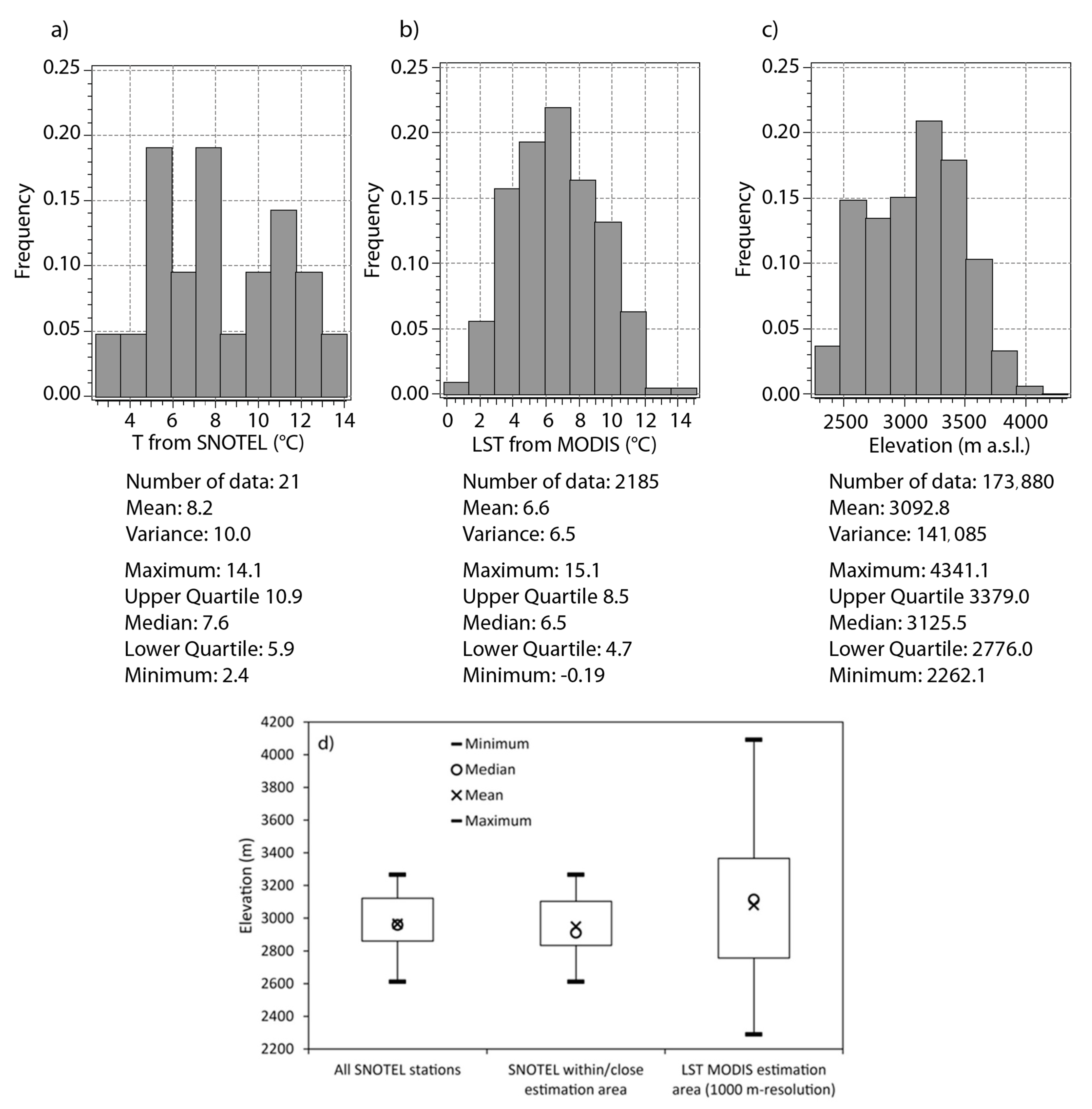
We combined temperature data from 21 SNOTEL stations, LST from MODIS (product MOD11A1), and elevation data to generate temperature fields in RMNP. The elevation data were obtained from the National Elevation Dataset DEM of the United States Geological Survey available at <nationalmap.gov>. The spatial resolution is one-third arc-second (about 10 m). It was upscaled to the two spatial resolutions employed in this study (100 m for the kriging based approaches and around 1000 m for the LST product and lapse rate based technique). The comparison between the kriging-based techniques and LST data and the hypsometric interpolation was done with 1000 m resolution data. Note that the selected resolution of around 1000 m corresponds to the spatial resolution of the MODIS LST product. Figure 2c shows the histogram and the statistics of the elevation data for the considered estimation area and its spatial distribution is showed in Figure 1. The selected SNOTEL stations (Figure 1) are located over an elevation range of 2612–3265 m a.s.l. The data are available from the U.S. Natural Resources Conservation Service (NRCS) at <wcc.nrcs.usda.gov> [34].
The MODIS LST product has a spatial resolution of around 1 km using a sinusoidal projection and temporal resolution of one-half day (providing daytime and nighttime data) [18]. The temporal coverage of this product is from 24 February 2000 to the present. The tile of MODIS that corresponds with the studied area is h09v04. The statistics of the temperature data in the days selected for this work are showed in Table 1.
We assume that the changes in the temperature data within the day due to the different time in which they were taken (for SNOTEL and MODIS) are insignificant. The time differences vary from 6 to 18 min. On the other hand, the MODIS LST data are used as secondary information. The LST values are not incorporated in the estimations. The proposed geostatistical approaches uses the spatial correlation between the target and secondary variables. Therefore, the estimation time corresponds to the SNOTEL data collection time. The data for the first day were used to apply the complete proposed methodology and the others were employed to evaluate it. Note that we have selected one day in each season of the year.
On 10 September 2018, the mean SNOTEL temperature for the 21 SNOTEL stations was 8.2 °C and the standard deviation 3.2 °C (see Figure 2a). Due to the scarce air temperature data in our case study, secondary information from LST and elevation is included to generate the estimated fields. Over the estimation area, 2185 pixels of MODIS LST product are included. The mean and the standard deviation of these data are 6.6 °C and 2.5 °C, respectively, with a Gaussian distribution (see Figure 2b). The mean and standard deviation of the temperature for the other days are included in Table 1. The range of elevation of the study area is 2262 to 4241 m a.s.l. (see Figure 2c). It is covered by the LST product, meanwhile the elevation range for SNOTEL is more limited (Figure 2d).

3. Methodology

We propose to start assessing the correlation coefficient (R2) of the linear correlation between air temperature and the secondary data (elevation and MODIS LST). It informs how secondary data can contribute to the final maps of temperature, in terms of performance. We also compared the two direct solutions for air temperature characterization, the MODIS LST which is obtained directly from the product MOD11A1 and the hypsometric interpolation. The hypsometric interpolation was obtained at the same resolution as MODIS LST by applying the lapse rate estimated from the SNOTEL stations located within or close to the study domain. It uses the linear correlation between elevation and air temperature to interpolate in a grid that covers the study area.
In the case of the kriging-based approaches, the study area (Figure 1) was divided into a finite number of cells (173,880), of 100 m resolution, employed to obtain temperature fields using seven geostatistical approaches: OK that only uses SNOTEL temperature measurements to obtain the temperature fields, KED and COK using elevation as secondary data, KED and COK using MODIS LST as secondary data, and merged solutions of KED and COK using both sources of secondary data (see Table 2). Theoretical details about the different approaches can be found in Appendix A. The obtained estimates were upscaled and compared with the MODIS LST map and the hypsometric interpolation at the spatial support of 1 km, studying the correlation between them and considering the uncertainty of the kriging estimations. The comparisons were established between the value obtained with the more direct solutions (LST from MODIS and the hypsometric interpolation) and the range of values defined by the kriging-based estimates ± σ (standard deviation of the estimation). We calculated the percentage of cells that are within the cited range of uncertainty. Finally, we also analyze the performance of the different applied geostatistical approaches through a cross validation experiment, considering the SNOTEL temperature measurements.
Air temperature is a spatially continuous variable that changes gradually. Considering this assumption, the variogram is the habitual way to quantify the spatial correlation in geostatistical estimations. In this work we employed several geostatistical techniques (OK, KED, and COK) and merged solutions of them to obtain temperature fields. Note that these techniques do not use regression models calibrated previously. They use data of the target and explanatory variables and information about the spatial correlation of them quantified by using the variogram. The experimental variograms employed with these approaches have been adjusted using one of the next models: spherical, exponential, and Gaussian [35]. The first approach that we considered is OK, which is the most widely used kriging method [36]. It estimates a value at a point of a region using information of the spatial continuity of the target variable through the variogram and data in the neighborhood. OK uses only data of the target variable and distance. In cases where a high amount of data is available this can be enough, but, in our case study, scarce data of temperature measurements are available. In addition to this data we also know that there is an elevation-based variance and a correlation between air temperature and LST. This information is very useful to improve our estimations by using KED and COK.
In KED the mathematical expected value of the target variable is expressed as a polynomial function of the drift variable [37]. The kriging system is performed by inserting additional constraints (one by each degree of the polynomial function) into the OK system. In this study, elevation and MODIS LST are the drift variables and the selected function is linear (one additional constraint). The selection of the function requires a previous analysis of the correlation between the target and the drift variables. The mean elevation must be known at the experimental location and the estimated grids. COK calculates estimates or predictions for a poorly sampled variable (in our case temperature) with help of a well-sampled variable (in our case elevation or LST from MODIS) [38]. The variables (target and secondary) should be highly correlated (in a positive or negative way).
We also explored the combination of both secondary variables (elevation and LST from MODIS) through merging estimates. In this way the merged KED is performed by combining the KED using elevation, and the KED using LST and the merged COK, defined by combining COK using elevation and COK using LST. The merging is carried out by calculating a weighted average of the estimates using weights that are inversely related to the estimation variance on the individual estimates. In the same way, the associated estimation variance is calculated as the product of the individual estimation variances divided by the sum of them [39].
The performance of the seven considered kriging-based solutions (OK, KED using elevation, KED using MODIS LST, COK using elevation, COK using MODIS LST, merged KED (obtained by merging KED using elevation and KED using MODIS LST) and merged COK (obtained by merging COK using elevation and COK using MODIS LST)) have been assessed by using a cross validation experiment. Theoretical details about the cross validation experiment can be found in Appendix B. It can be used for checking the effect of different kriging neighborhoods, different types of variogram models, different sets of variogram parameters for the same type of model or different geostatistical approaches [38]. In the cross-validation methodology, each experimental datum is dropped from the experimental data set in turn and is calculated from the remaining experimental data, information about explanatory variables (in the case of multivariate approaches) and information its spatial correlation from the variogram [40]. Thus, it is possible to determine the true error of the interpolation by kriging. We also calculated the squared error and the standardized squared error by using the kriging variance.
As commented in Section 2, the proposed methodology was applied to the assessment of the temperature in the first selected day and evaluated with the other days. The evaluation was performed by analyzing four days, each in different seasons, using the estimation obtained with the two best techniques identified for the first day.

4. Results

4.1. Application of the Methodology

The application of all methods was for the time point 10 September 2018 at 22:00.

4.1.1. Analysis of the Secondary Information

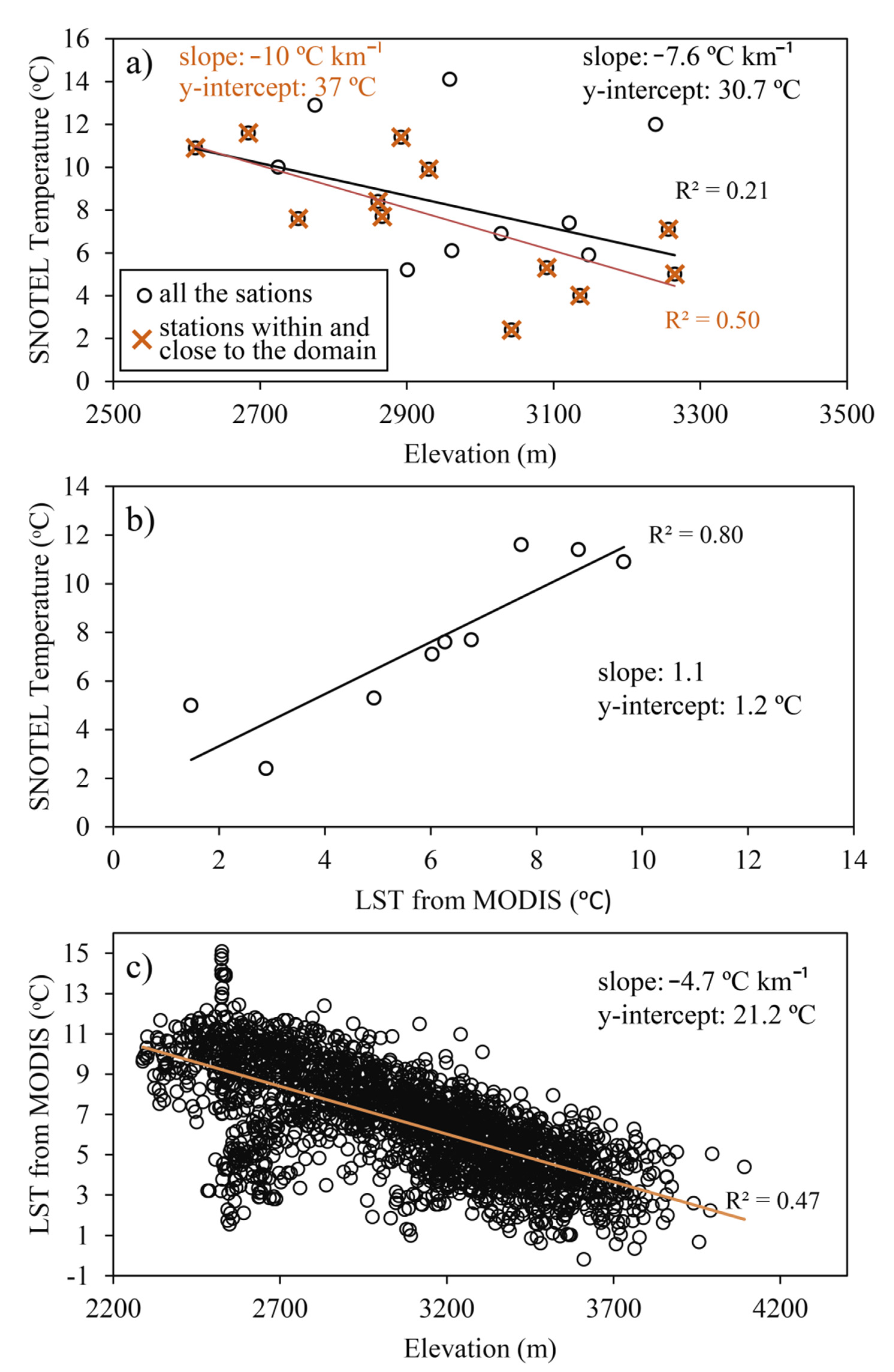
SNOTEL temperature decreases with elevation but the correlation between both variables is moderate; the R2 of the linear relationship is 0.21 for the whole domain and 0.50 for the estimation area (see Figure 3a). Similar results were found for this study area in a previous analysis [8]. The scarce air temperature data from SNOTEL were complemented by well-sampled secondary information from elevation and LST in order to obtain air temperature fields. In the same way LST decreases with elevation (Figure 3c) and the R2 of these variables is slightly higher (R2 of 0.47). In the case of LST from MODIS the correlation with SNOTEL temperature is good (R2 of 0.80) (see Figure 3b). At first sight MODIS LST temperature should provide better results as secondary variable in the estimations. However, some temperature data can be explained by elevation and its incorporation can complement the data provided by MODIS LST.
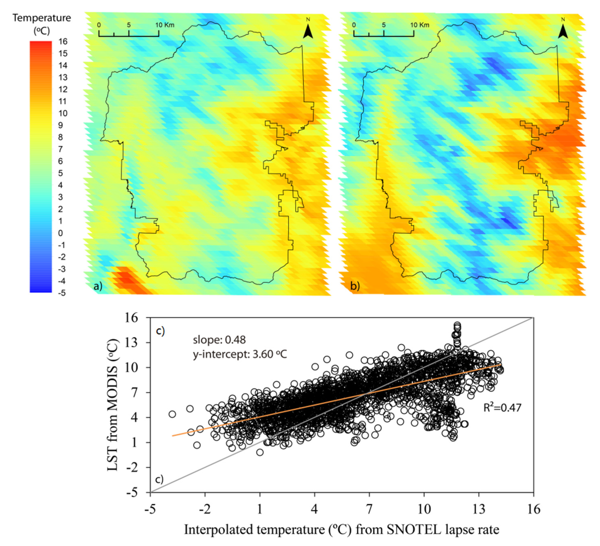
It should be noted that the spatial distribution of LST from MODIS pixels are parallelograms (Figure 4a) due to the original sinusoidal projection has been projected to the WGS 1984 projection. In general, lower LST are related to higher elevation (see Figure 1 and Figure 4a). An additional relatively direct solution can be obtained by applying the lapse rate obtained from SNOTEL stations (slope −10 °C km−1 and y-intercept 37 °C (see Figure 3a)) to the elevation distribution (see Figure 4b). The R2 between both solutions is 0.47. Below the threshold of 7 °C the LST solution shows higher values than the hypsometric approach (see Figure 4c). Both, LST and hypsometric interpolation solutions should be used with caution. LST shows a good correlation with air temperature, although they are different variables, and the correlation of temperature and elevation is moderate in our case study (see Figure 3a).

4.1.2. Estimation by Using Geostatistical Approaches

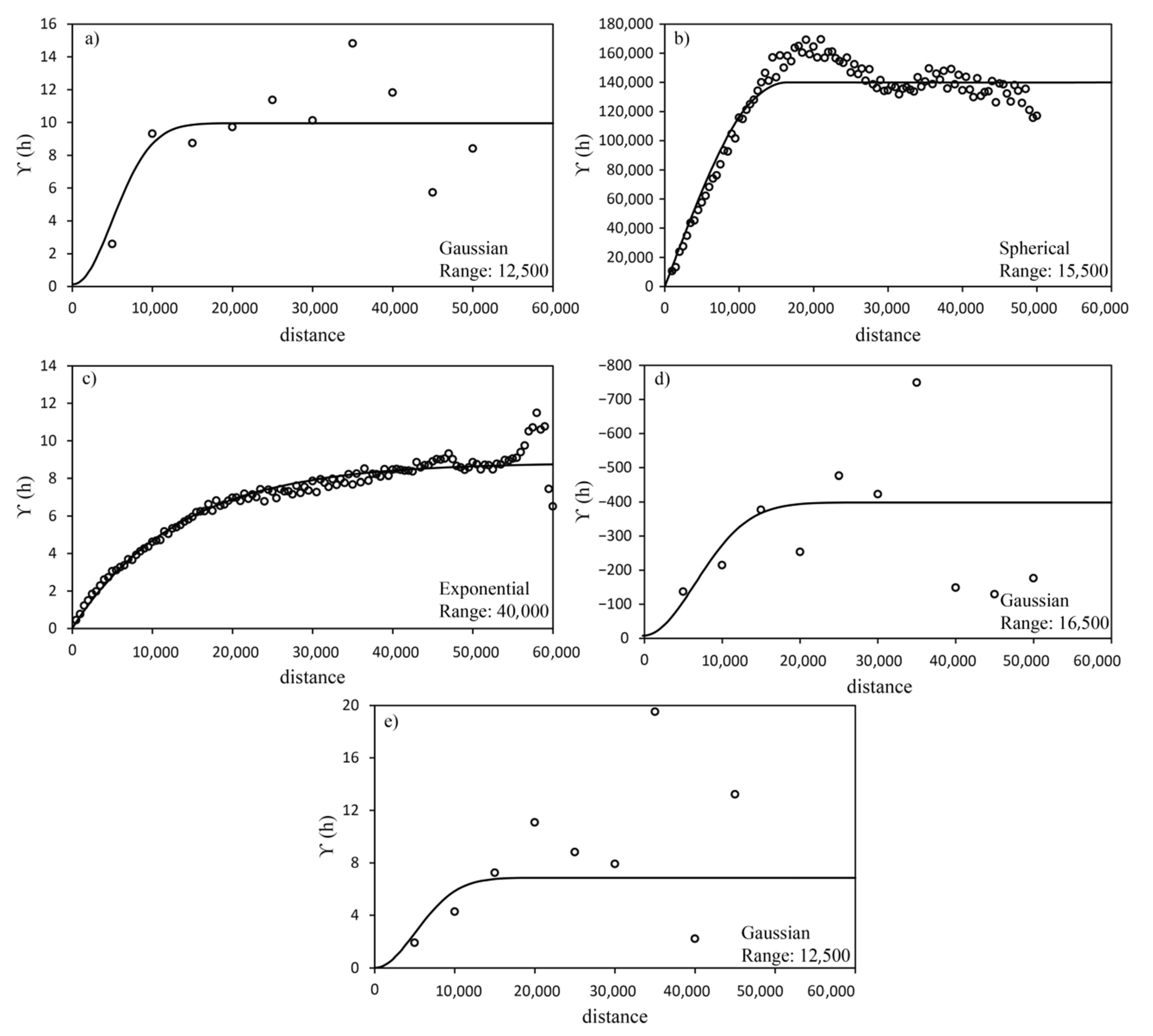
An alternative to the previous solution is obtained by using kriging-based methodologies. The different geostatistical techniques presented in Section 3 requires including the spatial correlation in the estimations through the direct and cross variograms of the target and secondary variables. OK and KED use direct variograms and COK use direct and cross variograms. The variograms model employed for SNOTEL data, elevation data and LST from MODIS are Gaussian, Spherical, and Exponential, respectively (See Figure 5a–c respectively). The sill employed to adjust the direct variograms are close to the variance of the data (see Figure 2) and the ranges are 12,500 m for SNOTEL data, 40,000 m for LST from MODIS, and 15,500 m for elevation. For the cross variograms of SNOTEL data with elevation and SNOTEL data with LST from MODIS, the Gaussian variogram was selected and the ranges are 16,500 and 12,500 m, respectively.
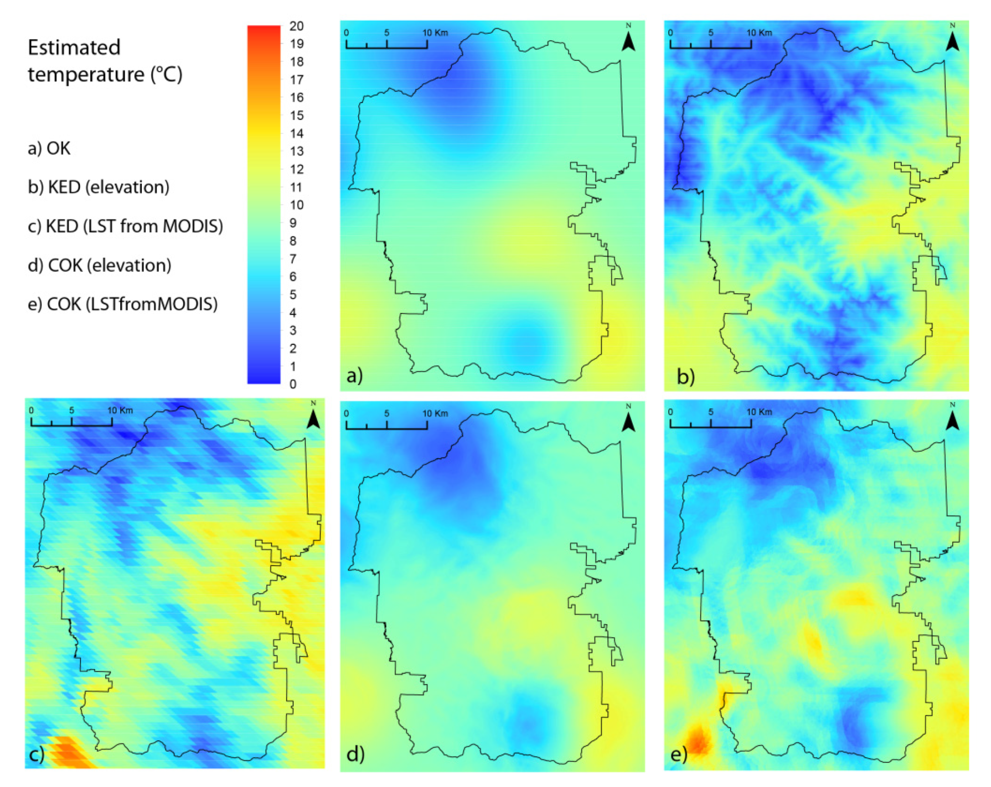
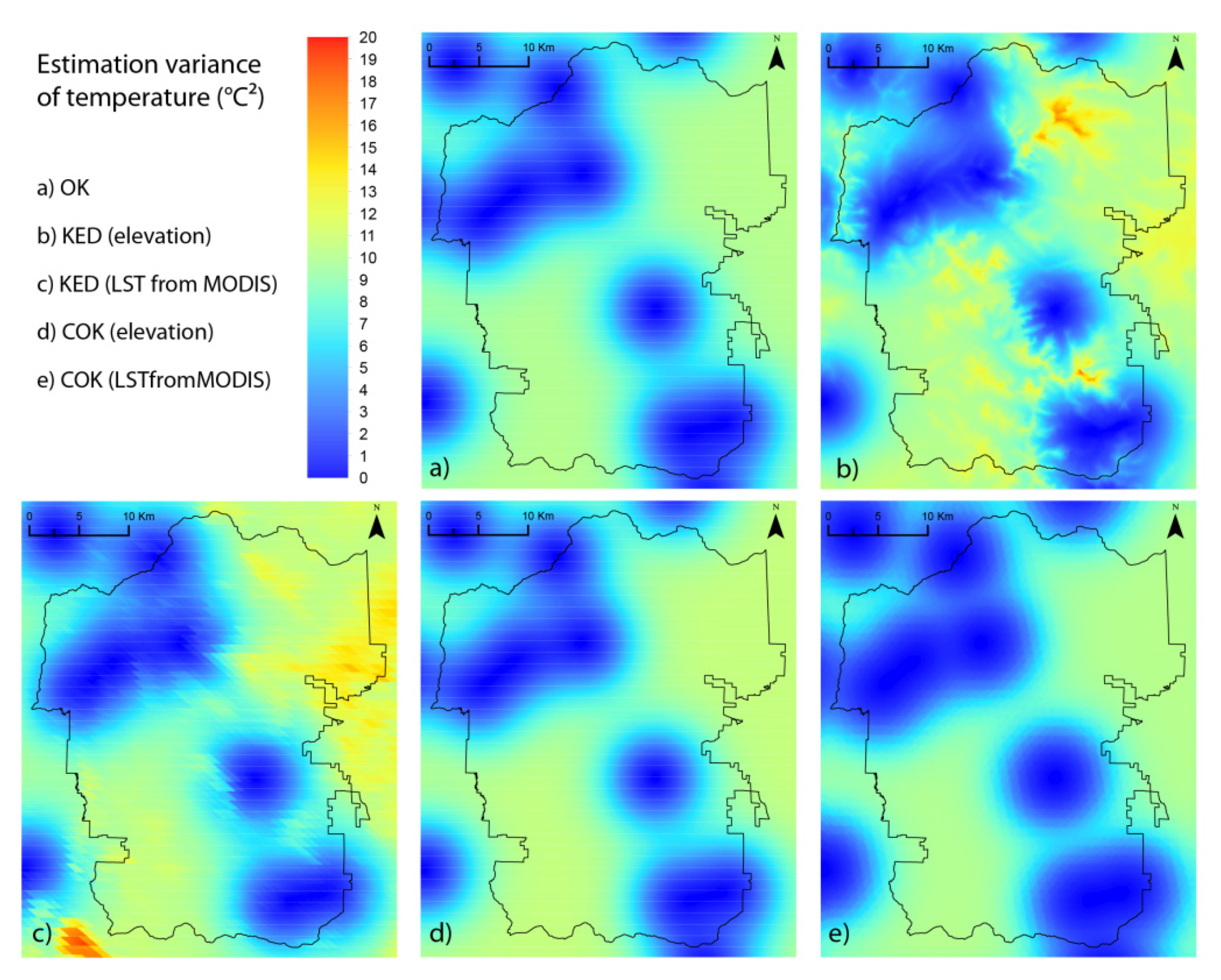
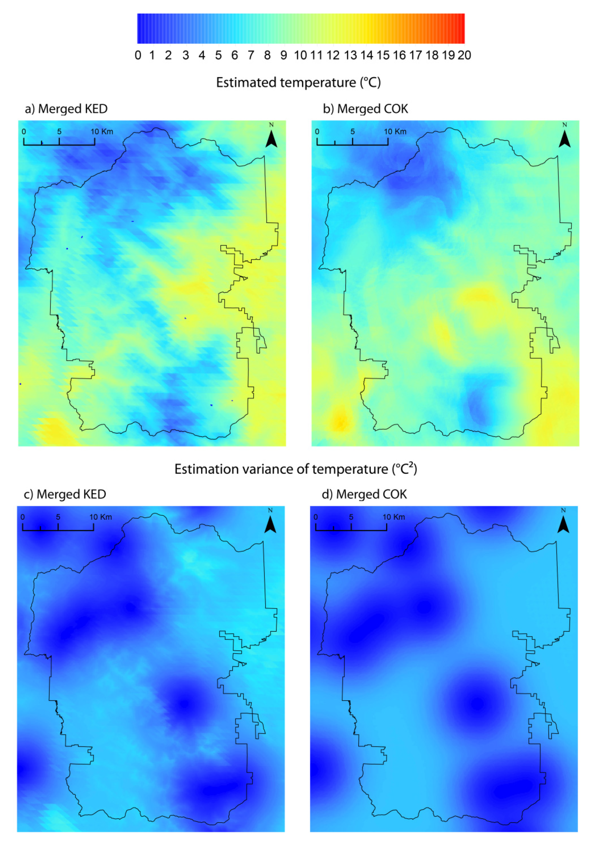
The resultant maps of temperature for RMNP by using OK, KED, and COK with elevation and MODIS LST solutions are showed in Figure 6. OK (Figure 6a) provides a simple smoothed map that only considers the scarce measurements. KED using elevation (Figure 6b) is very influenced by elevation. In this solution the hills (with lower temperature) and valleys (with higher temperature) can be distinguished. In the case of KED using MODIS LST (Figure 6c) the map is very similar to the LST map (see Figure 3a). On the other hand, COK (especially using elevation, see Figure 6d) provides maps more influenced by the air temperature measurements (more similar to OK). COK using MODIS LST provides a map that visually seems a mixed map between OK map and LST map (Figure 3a). The estimation variance is distributed very similarly for all the solutions (see Figure 7). Lower estimation variances are observed around the experimental locations. The estimates and variance of estimation of the merged KED, obtained as weighted average of KED using elevation and KED using LST MODIS LST, are showed in Figure 8a,c, respectively. Conversely, the maps of the estimates and variance of estimation of merged COK, obtained as weighted average of COK using the two sources of secondary data, are showed in Figure 8b,d, respectively.

4.1.3. Comparison of Geostatistical Estimations with MODIS LST and the Lapse Rate Solution

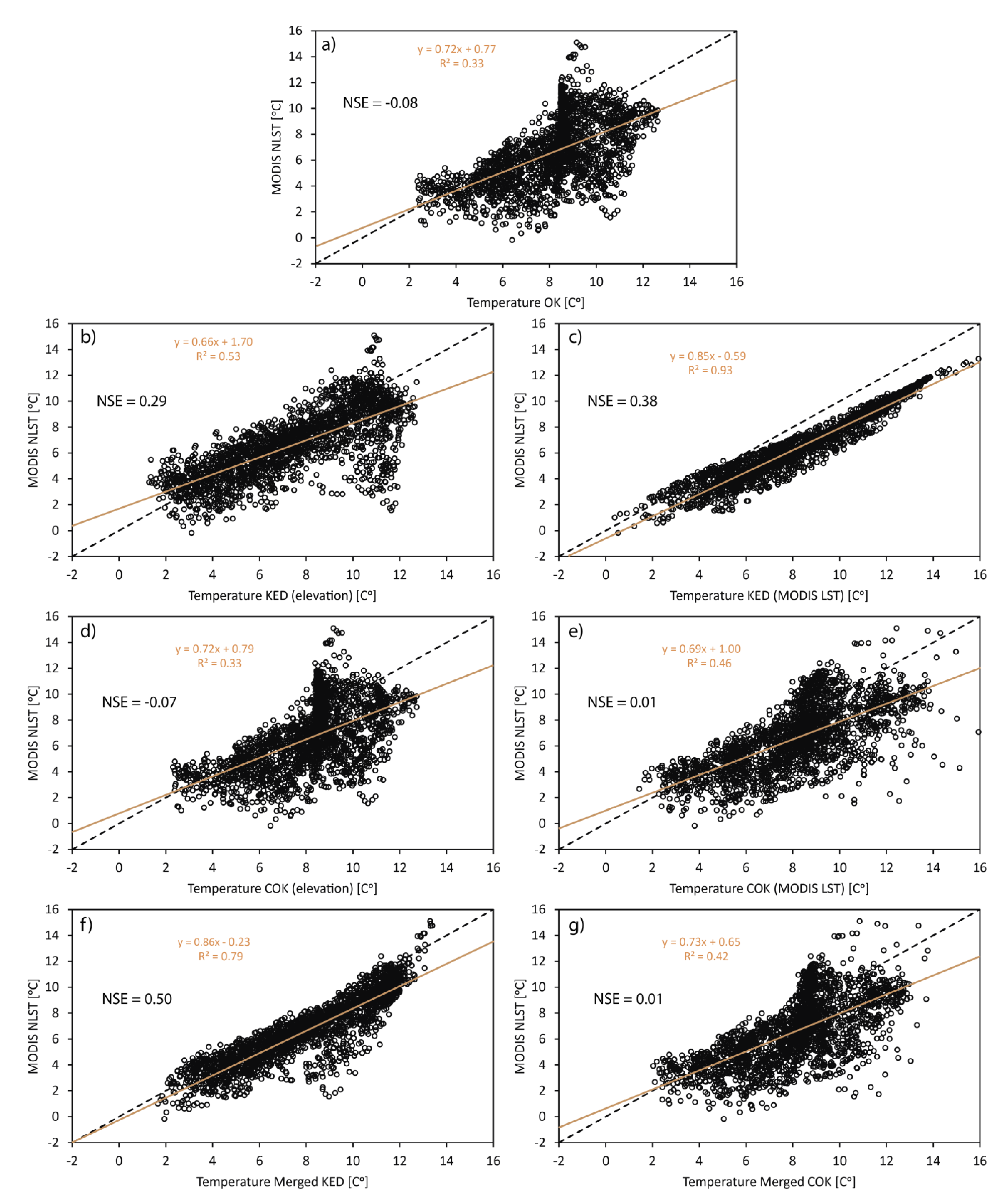
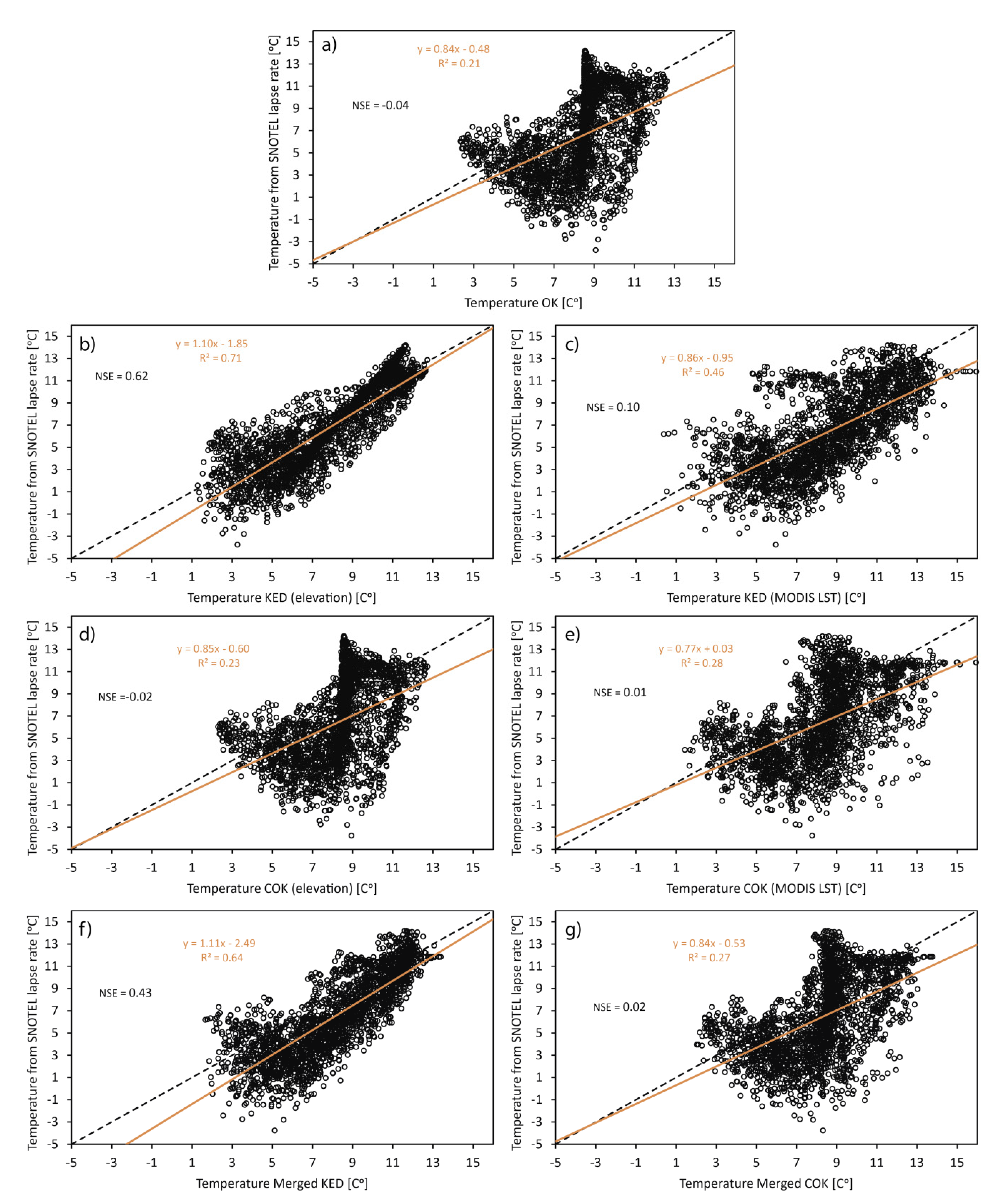
We compared the temperature maps obtained using the seven geostatistical solutions (Figure 6 and Figure 8) with the MODIS LST map (Figure 4a) and the interpolated temperature using the lapse rate from SNOTEL (hypsometric data) (Figure 4b). We compared the R2 of the linear correlation between the different geostatistical approaches and the LST and interpolation using the SNOTEL lapse rate. We also studied the percentage of pixels of LST and interpolation using the SNOTEL lapse rate that are included in the estimation uncertainty range of the different geostatistical approaches (Table 3). The different maps obtained with 100-m resolution were upscaled to obtain estimates with the MODIS LST spatial support and compared pixel to pixel to the LST values (see Figure 9). All the estimates are positively correlated with the MODIS LST. The highest correlations (R2 of 0.93 and 0.79) are obtained for the KED using MODIS LST and the merged KED, which also considers MODIS LST data. The COK and merged COK (they also use data from MODIS LST) show lower correlations (R2 of 0.45 and 0.42, respectively). These R2 values are similar to those ones obtained by the geostatistical approaches that do not use MODIS LST for estimation. OK presents a R2 of 0.33. The R2 values for KED and COK, which only use elevation as secondary data, are 0.53 and 0.33, respectively. In the same way, the kriging-based estimates were compared to the hypsometric interpolation (Figure 10). The highest correlations (R2 of 0.71 and 0.64) are obtained for the KED using elevation and the merged KED. Both of them include elevation in the estimation procedure. COK and merged COK (they also use data from elevation) show lower correlations (R2 of 0.23 and 0.27, respectively). The correlation with the techniques that do not use elevation in the estimation procedure is low (R2 of 0.21 for OK, 0.46 for KED using LST and 0.28 for COK using LST).
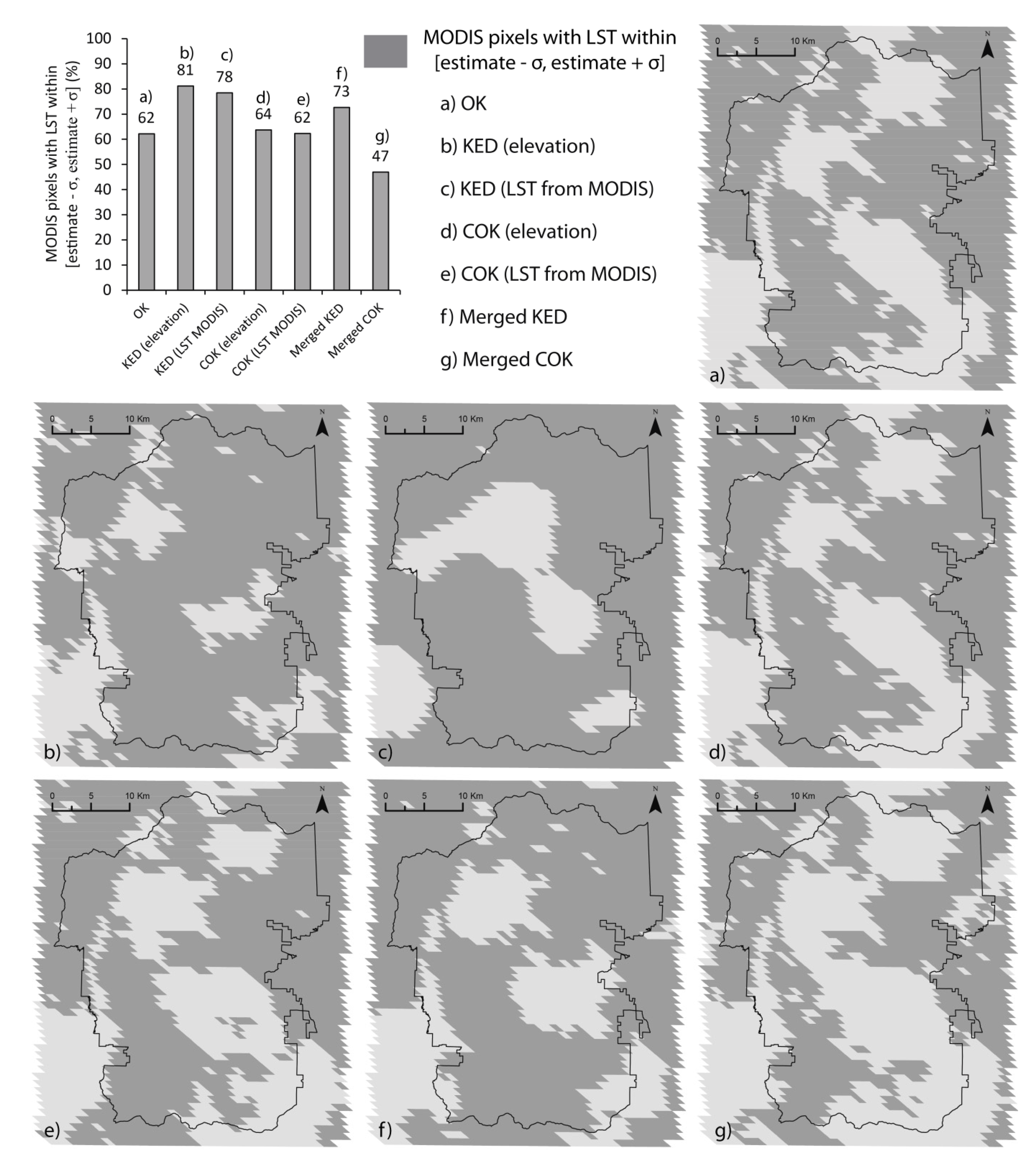
The geostatistical solutions were also compared with MODIS LST and the hypsometric interpolation considering the estimation variance of kriging-based techniques. The estimation variance is a measure of the estimation uncertainty and is expected that the true value of the estimated variable is between the range from estimate −σ to estimate + σ (σ is the standard deviation of the estimation). Figure 11 shows the pixels that fulfill this condition for each of the geostatistical solutions compared to MODIS LST. In this comparison, the solutions that show the highest agreement with MODIS LST are not those ones that use LST for estimation. In both cases, KED and COK, the percentage of pixels in the range (from estimate −σ to estimate + σ) is higher when elevation is used as secondary data (81% vs. 78% for KED, and 64% vs. 62% for COK). These coincidence percentages are 73%, 47% and 62% for merged KED, merged COK and OK, respectively. In the hypsometric interpolation (Figure 12), the number of pixels with values between the range (from estimate −σ to estimate + σ) is in general lower. Nevertheless, as for LST, in both cases, KED and COK, the percentage of pixels where the condition is fulfilled grows when elevation is used as secondary data (50% vs. 38% for KED and 40% vs. 38% for COK). These percentages are 35%, 30%, and 40%, for merged KED, merged COK and OK, respectively.

4.1.4. Cross Validation Experiment for Geostatistical Approaches

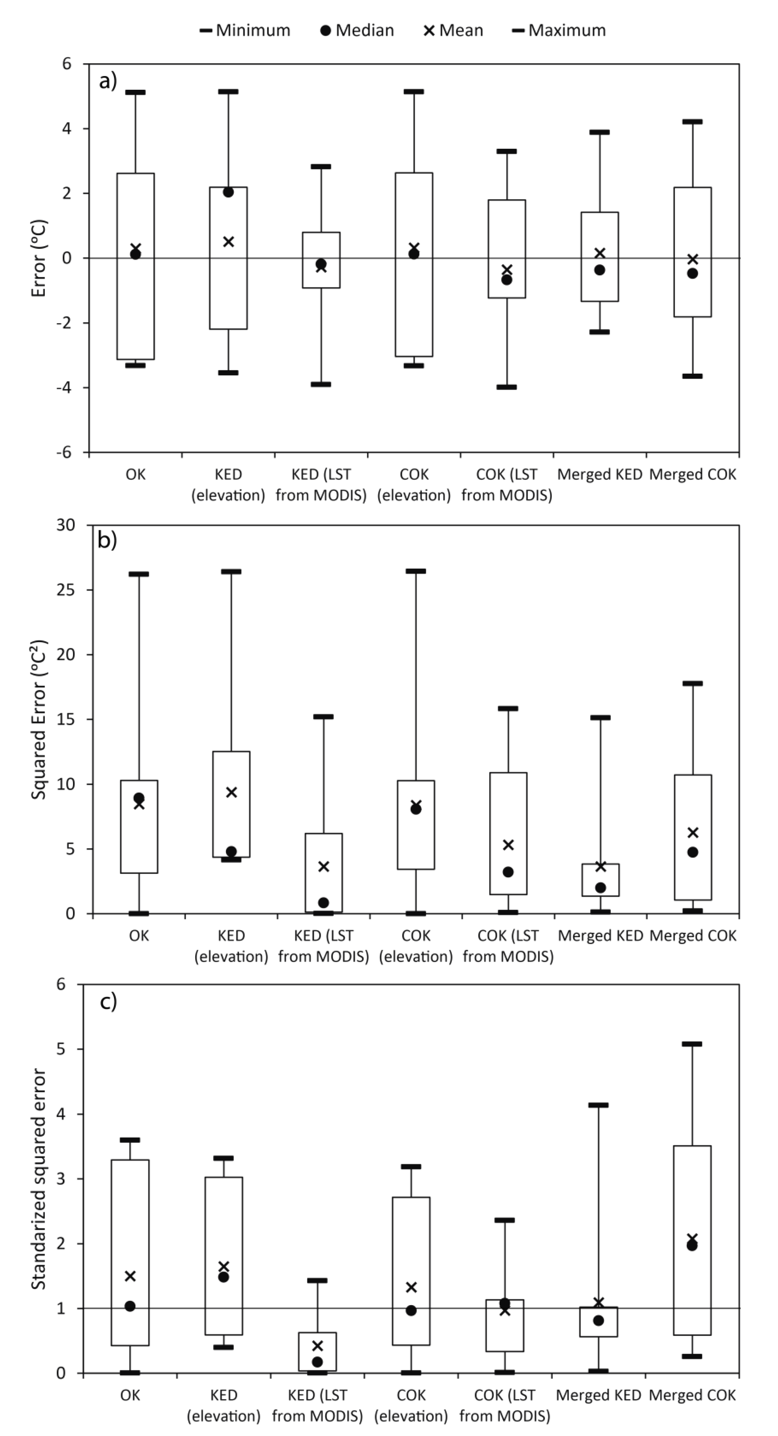
Finally, we assessed the performance of the geostatistical approaches by using a cross validation experiment (see Section 3). Figure 13 includes the box whiskers of error, square error, and standardized square error. Considering the mean error, merged COK and merged KED show the best results (0.03 and 0.16 °C, respectively). However mean error could include large positive and negative errors that are offset. In this case, the mean square error is a better performance statistic. Merged KED and KED using MODIS LST show the lowest values of mean square error (3.84 and 3.66 °C, respectively). Conversely, if we want to know how well (statistically) the kriging variance is, we must consider the mean standardized squared error. In this case, COK using MODIS LST and Merged KED show the best results (0.97 and 1.02, respectively). In view of these three performance statistics, we can conclude the merged KED is the best estimation technique for the case study. It includes secondary data from elevation and MODIS LST that complement the scarce air temperature measurements. In this study KED shows better results with respect COK attending to the cross validation experiment. The same conclusion was obtained by Pardo-Igúzquiza for precipitation estimation [41].

4.2. Validation of the Methodology

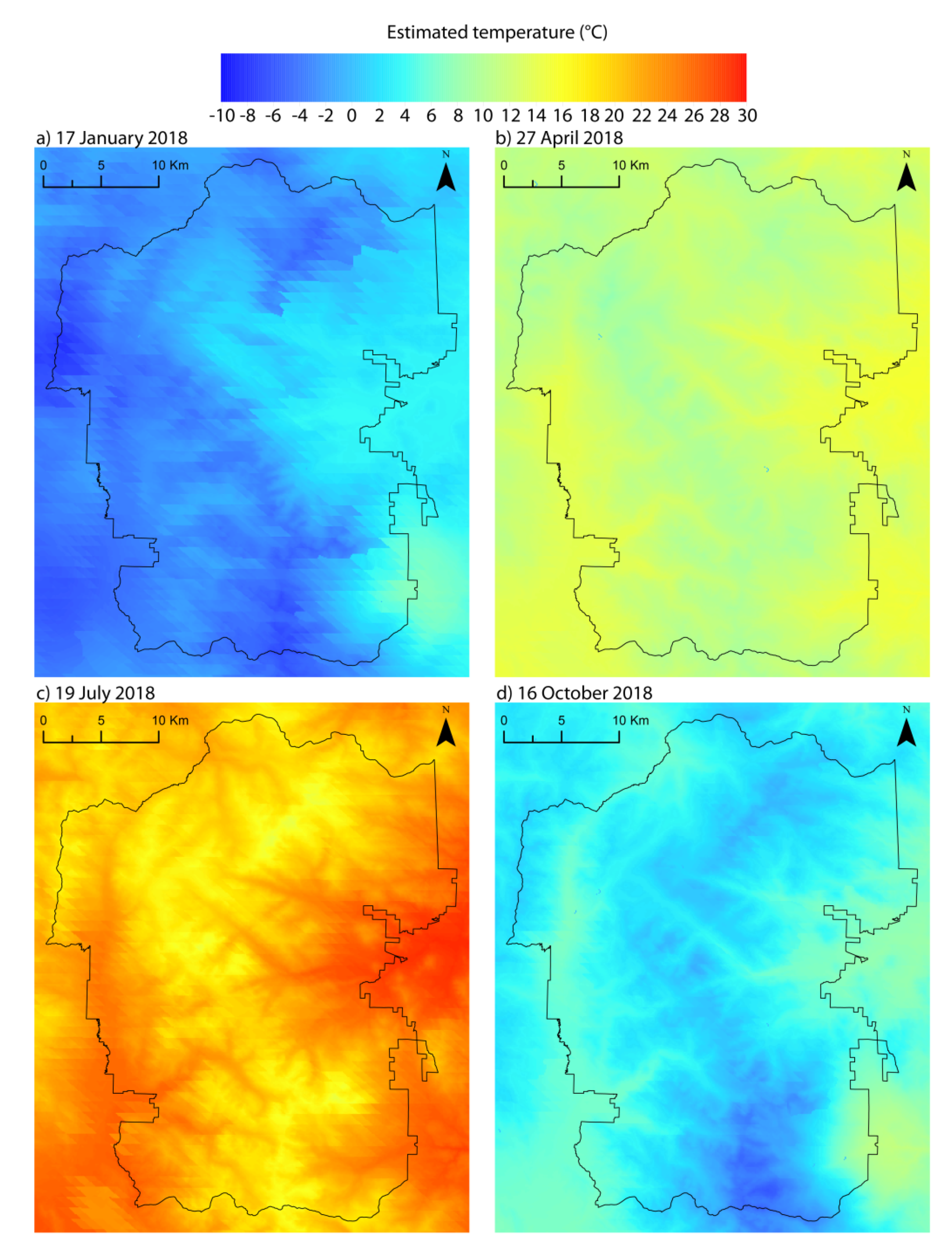
Merged KED and KED using LST are the two best solutions obtained in the application of the methodology (previous section). They and the KED using elevation, which is used to obtain the merged KED, were evaluated by using a cross validation experiment in four days of different seasons (see Table 1). Note that we considered the same range of the variograms obtained for the first day (10 September 2018) employed in Section 4.1, but the sill of the variogram was updated according to the data of each day. The mean squared error for KED using elevation, KED using LST, and merged KED is 4.1, 6.6, and 3.6 °C2, respectively. Again, the best solution is the merged KED. The maps of temperature obtained by using this technique are included in Figure 14. For the different seasons, the estimated temperature varies from −8.2 to 20.1 °C. The mean and standard deviation of the estimated temperature across the study area for the specific days are showed in Table 4. The minimum and maximum mean temperatures and the higher values of standard deviation are associated with the winter and summer days.

5. Discussion

In cases with data scarcity, secondary information, which is well-sampled and correlated with the target variable, is crucial to know the spatial distribution of land surface or near surface variables [42]. In our case study, due to the moderate correlation of temperature with elevation (R2 of 0.50), the hypsometric interpolation is not accurate enough. Conversely, despite the good correlation of air temperature with LST (R2 of 0.80), they are different variables and LST should not be used directly to characterize air temperature patterns. The comparison between the different estimations of air temperature with LST showed considerable biases, as previously observed [8]. For the best estimation of air temperature in this study (merged KED), 73% of the MODIS pixels showed a value of LST within the stated uncertainty range (from estimate −σ to estimate + σ). While air temperature is a measure of how hot or cold the air is, the LST is the radiative skin temperature of the land surface measured in the direction of the remote sensor [17]. However, some studies have developed methodologies to calibrate hydrological models by using LST instead air temperature (e.g., [21,22]). These approximations should be used with caution since the physical processes that both variables can explain (e.g., evapotranspiration or snow melt) can be different depending on the study case. Yet, LST can be useful when it is used as secondary data to obtain air temperature fields as demonstrated in this study and previous research [28,43]. Here, we use similar methodologies (e.g., KED or COK) to include LST as secondary data, as have previously been done, and we include a new procedure to incorporate elevation together with LST as secondary data through weighted kriging solutions. This approach was used previously to merge precipitation estimations [39].
Both elevation and LST, can explain some aspects of the temperature variability and can be useful to obtain temperature fields by applying adequate techniques. In our case study the performance of the merged KED, which uses elevation and MODIS LST as secondary variables, is good with a root mean squared error (RMSE) of 1.96 °C. This value is 2.91 °C in the case of OK, which only uses temperature measurements. Other authors found that including secondary data improve the performance of estimations (e.g., when OK was compared to KED [44] or COK [45]). Different approaches must be tested when secondary data are included into the estimation procedures. For example, in our case study the KED using elevation shows poorer results than the OK (RMSE of 3.06 vs. 2.91 °C). This may be due to the relatively lower correlation between measured temperature and elevation. However, good results were obtained when elevation is considered together with MODIS LST through the merged KED. In the evaluation procedure using the other days, the merged KED also obtained the best results. In accordance with cross-validation statistics, in this study KED seems to give the most coherent results compared to COK. Other authors also found this approach as the best one in the estimation of precipitation [41]. Other cases studies showed COK performed slightly better when it is used to approach the groundwater table in aquifers [46]. Therefore, for each case study and target variable, both multivariate geostatistical techniques should be evaluated [47].
This work proposed different approaches to obtain air temperature fields from scarce measurements and well-sampled secondary data, and analyzed the differences between air temperature and LST. It also showed a comparison of the performance of geostatistical approaches. Despite the applicability of the methodology to this study area with data scarcity, the results could be more reliable by incorporating additional air temperature data. The proposed methodology can be used to estimate air temperature by using elevation and LST products with higher temporal resolution [48]. Note that products with higher temporal resolution are related to a lower spatial resolution (e.g., the hourly LST product of Copernicus Global Land Service has a temporal resolution of 4 h and a spatial resolution of 5 km compared to the MODIS LST product employed in this study that has a 12 h time step at a 1-km resolution). Other secondary data, such as the vegetation index [49], could be a potential explanatory variable to estimate air temperature. Further, the proposed methodology could be applied to other and/or multiple time points. Only one winter day was evaluated, and the presence of snow may influence air temperature and LST [50,51].

6. Conclusions

In this work we presented a general method applicable to any case study to generate air temperature fields from point data, a DEM and a LST product. The methodology is useful to estimate air temperature fields under data scarcity, as our case study, where a limited number of SNOTEL air temperature data are available in the RMNP area. We compared kriging-based solutions with more direct solutions such as using the LST directly or to interpolate using hypsometry (lapse rate). Considering that LST and air temperature are not the same variable, if LST is used directly, it should be applied with caution since the physical processes that they can explain may be different. Conversely, the hypsometric interpolated solution is accurate when temperature and elevation show good correlation.
We used OK and multivariate kriging techniques (KED and COK) and weighted averaged solutions of them to consider both elevation and LST data. A cross validation experiment was used to assess the performance of the different geostatistical solutions for the application and evaluation of the methodology. Merged KED, which uses elevation and LST as secondary data, showed the best results for our case study, with a mean squared error of 3.7 and 3.6 °C2 for the application and evaluation of the methodology, respectively. It was obtained combining two solutions of multivariate geostatistical techniques (KED using elevation and KED using LST) to estimate air temperature fields combining correlated and well-sampled data of elevation and LST.
Both variables, elevation and LST, can explain some aspects of the temperature variability. The temperature patterns can be better explained by using elevation or LST depending on the time point (for this the assessment of correlations is needed), but merged KED includes information from both sources depending on the estimation uncertainty. It makes merged KED a useful approach to estimate air temperature fields under data scarcity by using well-sampled information from LST and elevation.

Author Contributions

Conceptualization, A.-J.C.-L., S.R.F., E.P.-I., and D.P.-V.; methodology, A.-J.C.-L., S.R.F., E.P.-I., and D.P.-V.; software, A.-J.C.-L. and E.P.-I.; validation, A.-J.C.-L., S.R.F., E.P.-I., and D.P.-V.; formal analysis, A.-J.C.-L., S.R.F., E.P.-I., and D.P.-V.; investigation, A.-J.C.-L., S.R.F., E.P.-I., and D.P.-V.; resources, A.-J.C.-L., S.R.F., E.P.-I., and D.P.-V.; data curation, A.-J.C.-L., S.R.F., E.P.-I., and D.P.-V.; Writing—Original draft preparation, A.-J.C.-L., S.R.F., E.P.-I., and D.P.-V.; Writing—Review & Editing, A.-J.C.-L., S.R.F., E.P.-I., and D.P.-V.; visualization, A.-J.C.-L.; supervision, S.R.F., E.P.-I., and D.P.-V.; project administration, S.R.F. and D.P.-V.; funding acquisition, S.R.F. and D.P.-V. All authors have read and agreed to the published version of the manuscript.

Funding

This research has been partially supported by the SIGLO-AN project (RTI2018-101397-B-I00) from the Spanish Ministry of Science, Innovation and Universities (Programa Estatal de I+D+I orientada a los Retos de la Sociedad), the GeoE.171.008-TACTIC project from GeoERA organization funded by European Union’s Horizon 2020 research and innovation program and the Colorado State University Warner College of Natural Resources Mountain Campus Research Support Fund (created by Professor James R. Meiman) that initiated this work.

Institutional Review Board Statement

Not applicable.

Informed Consent Statement

Not applicable.

Data Availability Statement

The SNOTEL temperature data were obtained from the Natural Resources Conservation Service <wcc.nrcs.usda.gov>. The MODIS land surface temperature data (product MOD11A1) were retrieved from the NASA Distributed Active Archive Center (DAAC) <earthdata.nasa.gov>. The digital elevation model was retrieved from the United States Geological Survey National Elevation Dataset <nationalmap.gov>.

Conflicts of Interest

The authors declare no conflict of interest. The funders had no role in the design of the study; in the collection, analyses, or interpretation of data; in the writing of the manuscript, or in the decision to publish the results.

Appendix A. Geostatistical Approaches

Air temperature is a variable with spatial continuity. The variable changes gradually. Considering this assumption, the variogram is the habitual way to quantify the spatial correlation. The variogram for a given variable can be expressed as
γ ( h ) = 1 2 n ( h ) i = 1 n ( h ) [ z ( s i ) z ( s i + h ) ] 2
where γ ( h ) is the experimental variogram,   h   is the step or distance, n ( h ) is the number of steps, and z ( s i ) is the variable value at the location s i . Normally, the experimental variogram is adjusted using one of the next models: spherical (Equation (A2)), exponential (Equation (A3)) and Gaussian (Equation (A4)).
γ ( h ) = C [ 3 2 h a 1 2 ( h a ) 3 ]
γ ( h ) = C [ 1 e ( h a ) ]
γ ( h ) = C [ 1 e ( h a ) 2 ] .
where a and C are the range and variance, respectively.
Considering a case study with area A divided in N grids of equal area B , the mean value of the target variable variable z B ( x i ) can be expressed as
z B ( x i )   = 1 B B ( x i ) z ( x ) d x
where z ( x ) is the mean of the target variable in the location x . The value of the target variable is known in the point being considered and we want to know it in the points of the grid.
Kriging methods provide estimates for Equation (A5) using the experimental data:
z B ( x i ) = j = 1 n λ j . z ( x j )

Appendix A.1. Ordinary Kriging (OK)

In OK the estimate z B ( x i ) is calculated solving Equation (A6) where the weights λ j are obtained by solving the OK system:
{ j = 1 n λ j . γ P   ( x i , x j ) + µ = γ ¯ P ( x i ,   B ( x o ) )   i = 1 , , n j = 1 n λ j = 1  
and the estimation variance is given by
σ ^ 2 = j = 1 n λ j . γ ¯ P ( x i ,   B ( x o ) ) + µ
where µ is the Lagrange multiplier, γ P   ( x i , x j ) is the variogram function for the points x i and x j , and γ ¯ ( x i ,   B ( x o ) ) is the mean variogram function between point x i and support B with centroid x o .
This technique uses only information of the target variable to estimate. The following techniques include also secondary information to estimate.

Appendix A.2. Co-Kriging (COK)

In COK the estimate of z B ( x i ) is given by
z B ( x i ) = j = 1 n λ j . z ( x j ) + j = 1 m ƞ j . y ( x j )
where y ( x j ) are experimental data on a correlated secondary variable. The weights λ j and ƞ j are obtained as solution of the COK system:
{ j = 1 n λ j . γ P   ( x i , x j ) + j = 1 m ƞ j . γ P Y   ( x i , x k ) + µ 1 = γ ¯ P ( x i ,   B ( x o ) )   i = 1 , , n j = 1 n λ j . γ P Y   ( x k , x j ) + j = 1 m ƞ j . γ Y   ( x i , x k ) + µ 1 = γ ¯ P Y ( x k ,   B ( x o ) )   i = 1 , , n j = 1 n λ j = 1 j = 1 m ƞ j = 1
and the estimation variance is given by
σ ^ 2 = j = 1 n λ j . γ ¯ P ( x i ,   B ( x o ) ) + j = 1 m ƞ j . γ ¯ P Y ( x k ,   B ( x o ) ) + µ 1
where µ 1 is the Lagrange multiplier, γ P ( h ) is the variogram function of the target variable,   γ P Y ( h ) is the cross-variogram of the target and secondary variable, and the bar over the variogram denotes the mean variogram between point x i or x k and support B with centroid x o .

Appendix A.3. Kriging with External Drift (KED)

In KED the mathematical expected value of the target variable mean random function Z ( x ) is expressed as a function of the drift variable Y ( x ) . Normally the function is linear and can be expressed as
E [ Z ( x ) ] = a 1 + a 2 Y ( x )
The target variable z B ( x i ) for the linear case, with weights λ j obtained as solutions of the KED system, is calculated as
{ j = 1 n λ j . γ P   ( x i , x j ) + µ 1 + µ 2 y ( x i ) = γ ¯ ( x i ,   B ( x o ) )   i = 1 , , n j = 1 n λ j . y ( x j ) = y ( x o ) j = 1 n λ j = 1
with estimated variance σ ^ 2 expressed as
σ ^ 2 = j = 1 n λ j . γ ¯ ( x i ,   B ( x o ) ) + µ 1 + µ 2 y ( x o )
where µ 1 and   µ 2 are the Lagrange multiplier, γ P   ( x i , x j ) is the variogram function for the points x i , and x j and γ ¯ ( x i ,   B ( x o ) ) is the mean variogram function between point x i and support B with centroid x o .
The values of the coefficients a 1 and a 2 are not needed for solving equation systems (A13). To apply KED it is not necessary to know them. However the mean secondary variable must be known at the experimental location and the estimated grids.

Appendix B. Cross Validation Methodology

The cross-validation methodology is used in geostatistics for assessing the performance of the spatial interpolation by kriging. It can be used for checking the effect of different kriging neighborhoods, different types of kriging, different kind of variogram models, or different sets of variogram parameters for the same type of model. In cross-validation, each experimental datum is dropped from the experimental data set in turn and is calculated from the remaining experimental data. Thus it is possible to determine the true error of the interpolation by kriging:
e ( u i ) = z ^ ( u i ) z ( u i )
where e ( u i ) is the true error in the estimate of the ith experimental datum, z ^ ( u i ) is the estimate of the variable of interest at the location of the ith experimental datum, and z ( u i ) is the true value of the experimental datum of the variable of interest at the ith experimental location.
Thus, if there are N experimental data, cross-validation will give a set of N true errors { e ( u i ) ,   i = 1 , , N } . From these errors, the following cross-validation statistics can be obtained: mean error (ME), mean squared error (MSE) and mean standardized squared error (MSSE).
ME is defined as the mean of the true errors:
M E = 1 N i = 1 N e ( u i )
The ME is the bias of the estimation, whose value should be around zero. This criterion should always be met because kriging is an unbiased estimator.
MSE is defined as the mean of the squared true errors:
M S E = 1 N i = 1 N e 2 ( u i )
The MSE is the accuracy of the estimate and the value should be as small as possible.
MSSE is defined as the mean of the standardized squared true errors:
M S S E = 1 N i = 1 N e 2 ( u i ) σ K 2 ( u i )
where σ K 2 ( u i ) is the kriging variance in the estimate of the ith datum.
The MSSE is the evaluation of how well (statistically) the kriging variance is a realistic measure of uncertainty. The value should be around 1 if the kriging variance is a good measure of uncertainty.

References

  1. Gentine, P.; Chhang, A.; Rigden, A.; Salvucci, G. Evaporation estimates using weather station data and boundary layer theory. Geophys. Res. Lett. 2016, 43, 11661–11670. [Google Scholar] [CrossRef]
  2. Sexstone, G.A.; Clow, D.W.; Fassnacht, S.R.; Liston, G.E.; Hiemstra, C.A.; Knowles, J.F.; Penn, C.A. Snow sublimation in mountain environments and its sensitivity to forest disturbance and climate warming. Water Resour. Res. 2018, 54, 1191–1211. [Google Scholar] [CrossRef]
  3. Barnhart, T.B.; Molotch, N.P.; Livneh, B.; Harpold, A.A.; Knowles, J.F.; Schneider, D. Snowmelt rate dictates streamflow. Geophys. Res. Lett. 2016, 43, 8006–8016. [Google Scholar] [CrossRef]
  4. Martinec, J. Snowmelt-Runoff model for stream flow forecasts. Hydrol. Res. 1975, 6, 145–154. [Google Scholar] [CrossRef]
  5. Huang, S.; Eisner, S.; Magnusson, J.O.; Lussana, C.; Yang, X.; Beldring, S. Improvements of the spatially distributed hydrological modelling using the HBV model at 1 km resolution for Norway. J. Hydrol. 2019, 577. [Google Scholar] [CrossRef]
  6. Pérez-Sánchez, J.; Senent-Aparicio, J.; Segura-Méndez, F.; Pulido-Velazquez, D.; Srinivasan, R. Evaluating Hydrological Models for Deriving Water Resources in Peninsular Spain. Sustainability 2019, 11. [Google Scholar] [CrossRef] [Green Version]
  7. Pape, R.; Löffler, J. Modelling Spatio-temporal near surface temperature variation in High Mountain landscapes. Ecol. Model. 2004, 178, 483–501. [Google Scholar] [CrossRef]
  8. Collados-Lara, A.-J.; Fassnacht, S.R.; Pulido-Velazquez, D.; Pfohl, A.K.; Morán-Tejeda, E.; Venable, N.B.; Pardo-Igúzquiza, E.; Puntenney-Desmond, K. Intra-day variability of temperature and its near-surface gradient with elevation over mountainous terrain: Comparing MODIS land surface temperature data with coarse and fine scale near-surface measurements. Int. J. Clim. 2020, 1–15. [Google Scholar] [CrossRef]
  9. Zhang, F.; Zhang, H.; Hagen, S.C.; Ye, M.; Wang, D.; Gui, D.; Zeng, C.; Tian, L.; Liu, J. Snow cover and runoff modelling in a high mountain catchment with scarce data: Effects of temperature and precipitation parameters. Hydrol. Process. 2014, 29, 52–65. [Google Scholar] [CrossRef]
  10. Joyce, A.; Adamson, J.; Huntley, B.; Parr, T.; Baxter, R. Standardisation of Temperature Observed by Automatic Weather Stations. Environ. Monit. Assess. 2001, 68, 127–136. [Google Scholar] [CrossRef]
  11. Shiklomanov, A.I.; Lammers, R.B.; Vörösmarty, C.J. Widespread decline in hydrological monitoring threatens Pan-Arctic Research. Eos Trans. Am. Geophys. 2002, 83, 13–17. [Google Scholar] [CrossRef]
  12. Liston, G.E.; Elder, K. A Meteorological Distribution System for High-Resolution Terrestrial Modeling (MicroMet). J. Hydrometeorpl. 2006, 7, 217–234. [Google Scholar] [CrossRef] [Green Version]
  13. Roostaee, M.; Deng, Z. Effects of Digital Elevation Model Resolution on Watershed-Based Hydrologic Simulation. Water Resour. Manag. 2020, 34, 2433–2447. [Google Scholar] [CrossRef]
  14. Hudson, G.; Wackernagel, H. Mapping temperature using kriging with external drift: Theory and an example from Scotland. Int. J. Clim. 1994, 14, 77–91. [Google Scholar] [CrossRef]
  15. Rolland, C. Spatial and seasonal variations of air temperature lapse rates in alpine regions. J. Clim. 2003, 16, 1032–1046. [Google Scholar] [CrossRef] [Green Version]
  16. Blandford, T.R.; Humes, K.S.; Harshburger, B.J.; Moore, B.C.; Walden, V.P.; Ye, H. Seasonal and synoptic variations in near-surface air temperature lapse rates in a Mountainous Basin. J. Appl. Meteorol. Clim. 2008, 47, 249–261. [Google Scholar] [CrossRef]
  17. Li, Z.-L.; Tang, B.-H.; Wu, H.; Ren, H.; Yan, G.; Wan, Z.; Trigo, I.F.; Sobrino, J.A. Satellite derived land surface temperature: Current status and perspectives. Remote Sens. Environ. 2013, 131, 14–37. [Google Scholar] [CrossRef] [Green Version]
  18. Wan, Z.; Hook, S. MOD11A1 MODIS/Terra Land Surface Temperature and the Emissivity Daily L3 Global 1km SIN Grid. NASA LP DAAC 2015. [Google Scholar] [CrossRef]
  19. Khorchani, M.; Vicente-Serrano, S.M.; Azorin-Molina, C.; Garcia, M.; Martin-Hernandez, N.; Peña-Gallardo, M.; El Kenawy, A.; Domínguez-Castro, F. Trends in LST over the peninsular Spain as derived from the AVHRR imagery data. Glob. Planet. Chang. 2018, 166, 75–93. [Google Scholar] [CrossRef]
  20. Janatian, N.; Sadeghi, M.; Sanaeinejad, S.H.; Bakhshian, E.; Farid, A.; Hasheminia, S.M.; Ghazanfari, S. A statistical framework for estimating air temperature using MODIS land surface temperature data. Int. J. Clim. 2017, 37, 1181–1194. [Google Scholar] [CrossRef]
  21. Corbari, C.; Mancini, M.; Li, J.; Su, Z. Can satellite land surface temperature data be used similarly to ground discharge measurements for distributed hydrological model calibration? Hydrol. Sci. J. 2015, 60, 202–217. [Google Scholar] [CrossRef]
  22. Corbari, C.; Huber, C.; Yesou, H.; Huang, Y.; Su, Z.; Mancini, M. Multi-Satellite Data of Land Surface Temperature, Lakes Area, and Water Level for Hydrological Model Calibration and Validation in the Yangtze River Basin. Water 2019, 11, 2621. [Google Scholar] [CrossRef] [Green Version]
  23. Molotch, N.P.; Fassnacht, S.R.; Bales, R.C.; Helfrich, S.R. Estimating the distribution of snow water equivalent and snow extent beneath cloud cover in the Salt–Verde River basin, Arizona. Hydrol. Process. 2004, 18, 1595–1611. [Google Scholar] [CrossRef]
  24. Zink, M.; Mai, J.; Cuntz, M.; Samaniego, L. Conditioning a hydrologic model using patterns of remotely sensed land surface temperature. Water Resour. Res. 2018, 54, 2976–2998. [Google Scholar] [CrossRef]
  25. Benavides, R.; Montes, F.; Rubio, A.; Osoro, K. Geostatistical modelling of air temperature in a mountainous region of Northern Spain. Agric. Meteorol. 2007, 146, 173–188. [Google Scholar] [CrossRef]
  26. Jimeno-Sáez, P.; Pulido-Velazquez, D.; Collados-Lara, A.-J.; Pardo-Igúzquiza, E.; Senent-Aparicio, J.; Baena-Ruiz, L. A Preliminary Assessment of the “Undercatching” and the Precipitation Pattern in an Alpine Basin. Water 2020, 12, 1061. [Google Scholar] [CrossRef] [Green Version]
  27. Bianchi, E.; Villalba, R.; Viale, M.; Couvreux, F.; Marticorena, R. New precipitation and temperature grids for northern Patagonia: Advances in relation to global climate grids. J. Meteorol. Res. 2016, 30, 38–52. [Google Scholar] [CrossRef]
  28. Yang, Y.Z.; Cai, W.H.; Yang, J. Evaluation of MODIS Land Surface Temperature Data to Estimate Near-Surface Air Temperature in Northeast China. Remote Sens. 2017, 9, 410. [Google Scholar] [CrossRef] [Green Version]
  29. Kitsara, G.; Papaioannou, G.; Retalis, A.; Paronis, D.; Kerkides, P. Estimation of air temperature and reference evapotranspiration using MODIS land surface temperature over Greece. Int. J. Remote Sens. 2018, 39, 924–948. [Google Scholar] [CrossRef]
  30. Goble, P. Colorado Climate, Colorado Encyclopedia. Available online: https://coloradoencyclopedia.org/article/colorado-climate (accessed on 7 October 2019).
  31. PRISM Climate Group. 30-Year Normal Mean Temperature. Northwest Alliance for Computational Science & Engineering (NACSE) 2015, Based at Oregon State University. Available online: https://prism.oregonstate.edu/normals/ (accessed on 13 November 2020).
  32. Fassnacht, S.R.; Patterson, G.G.; Venable, N.B.; Cherry, M.L.; Pfohl, A.K.; Sanow, J.E.; Tedesche, M.E. How Do We Define Climate Change? Considering the Temporal Resolution of Niveo-Meteorological Data. Hydrology 2020, 7, 38. [Google Scholar] [CrossRef]
  33. Kampf, S.K.; Fassnacht, S.R. Snow, Colorado Encyclopedia. Available online: https://coloradoencyclopedia.org/article/snow (accessed on 12 January 2020).
  34. Natural Resources Conservation Service. NRCS: National Water and Climate Center SNOTEL Data Network; U.S. Department of Agriculture: Washington, DC, USA, 2016. Available online: ww.wcc.nrcs.usda.gov/snow/ (accessed on 26 July 2020).
  35. Matheron, G. Principles of geostatistics. Econ. Geol. 1963, 58, 1246–1266. [Google Scholar] [CrossRef]
  36. Chiles, J.P.; Delfiner, P. Geostatistics: Modelling Spatial Uncertainty; Wiley: New York, NY, USA, 1999. [Google Scholar]
  37. Collados-Lara, A.-J.; Pardo-Igúzquiza, E.; Pulido-Velazquez, D.; Jiménez-Sánchez, J. Precipitation fields in an alpine Mediterranean catchment: Inversion of precipitation gradient with elevation or undercatch of snowfall? Int. J. Clim. 2018, 38, 3565–3578. [Google Scholar] [CrossRef]
  38. Pardo-Igúzquiza, E.; Chica-Olmo, M.; Atkinson, P.M. Downscaling cokriging for image sharpening. Remote Sens. Envrion. 2006, 102, 86–98. [Google Scholar] [CrossRef] [Green Version]
  39. Grimes, D.I.F.; Pardo-Igúzquiza, E.; Bonifacio, R. Optimal areal rainfall estimation using raingauges and satellite data. J. Hydrol. 1999, 222, 93–108. [Google Scholar] [CrossRef]
  40. Fassnacht, S.R.; Dressler, K.A.; Bales, R.C. Snow water equivalent interpolation for the Colorado River Basin from snow telemetry (SNOTEL) data. Water Resour. Res. 2003, 39, 1208. [Google Scholar] [CrossRef] [Green Version]
  41. Pardo-Igúzquiza, E. Comparison of geostatistical methods for estimating the areal average climatological rainfall mean using data on precipitation and topography. Int. J. Clim. 1998, 18, 1031–1047. [Google Scholar] [CrossRef]
  42. Cassiani, G.; Christakos, G. Analysis and Estimation of Natural Processes with Nonhomogeneous Spatial Variation Using Secondary Information. Math. Geol. 1998, 30, 57–76. [Google Scholar] [CrossRef]
  43. Vancutsem, C.; Ceccato, P.; Dinku, T.; Connor, S.J. Evaluation of MODIS land surface temperature data to estimate air temperature in different ecosystems over Africa. Remote Sens. Environ. 2010, 114, 449–465. [Google Scholar] [CrossRef]
  44. Carrera-Hernández, J.; Gaskin, S. Spatio temporal analysis of daily precipitation and temperature in the Basin of Mexico. J. Hydrol. 2007, 336, 231–249. [Google Scholar] [CrossRef]
  45. Guo, Q.; Zhang, M.; Yang, X.; Zheng, M. Spatial Interpolation of Monthly Mean Temperatures Based on Cokriging Method. In Advances in Computational Science and Computing. ISCSC 2018. Advances in Intelligent Systems and Computing, Tlemcen, Algeria, 1–3 October 2018; Xiong, N., Xiao, Z., Tong, Z., Du, J., Wang, L., Li, M., Eds.; Springer: Cham, Switzerland, 2019; p. 877. [Google Scholar] [CrossRef]
  46. Boezio, M.N.M.; Costa, J.F.C.L.; Koppe, J.C. Kriging with an external drift versus collocated cokriging for water table mapping. Appl. Earth Sci. 2006, 115, 103–112. [Google Scholar] [CrossRef]
  47. Wackernagel, H. Multivariate geostatistics: An introduction with applications. Multivariate Geostatistics: An Introduction with Applications. J. Am. Stat. Assoc. 1996, 91, 1375. [Google Scholar] [CrossRef]
  48. Freitas, S.C.; Trigo, I.; Macedo, J.; Barroso, C.; Silva, R.; Perdigao, R. Land Surface Temperature from multiple geostationary satellites. Int. J. Remote Sens. 2013, 34, 3051–3068. [Google Scholar] [CrossRef]
  49. Jin, K.; Wang, F.; Zong, Q.L.; Qin, P.; Liu, C.X. Impact of variations in vegetation on surface air temperature change over the Chinese Loess Plateau. Sci. Total Envrion. 2020, 716, 136967. [Google Scholar] [CrossRef] [PubMed]
  50. Musacchio, C.; Coppa, G.; Merlone, A. An experimental method for evaluation of the snow albedo effect on near-surface air temperature measurements. Meteorol. Appl. 2019, 26, 161–170. [Google Scholar] [CrossRef] [Green Version]
  51. Thiebault, K.; Young, S. Snow cover change and its relationship with land surface temperature and vegetation in northeastern North America from 2000 to 2017. Int. J. Remote Sens. 2020, 41, 8453–8474. [Google Scholar] [CrossRef]
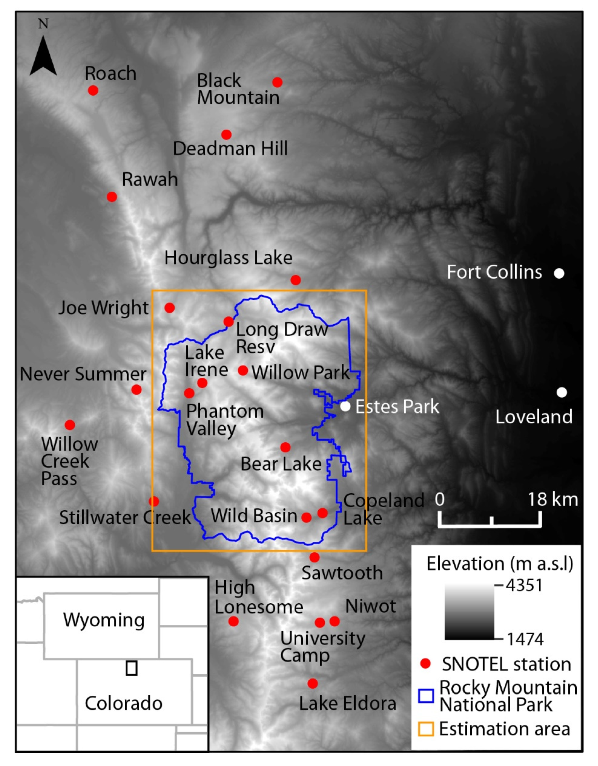
Figure 1. Location of the Rocky Mountain National Park, area of estimation and SNOTEL stations considered, and elevation map of the area.
Remotesensing 13 00113 g001
Figure 2. Histogram of the three sources of data for the 10 September 2018: (a) SNOTEL stations, (b) land surface temperature (LST) from MODIS, (c) elevation, and (d) box-whiskers of the elevation distribution for SNOTEL stations and LST from MODIS pixels.
Remotesensing 13 00113 g002
Figure 3. Correlation between the three sources of data: (a) SNOTEL temperature versus elevation, (b) SNOTEL temperature versus LST from MODIS, (c) LST from MODIS versus elevation.
Remotesensing 13 00113 g003
Figure 4. Spatial distribution (a) of LST from MODIS for the considered view time (21:54), (b) of the interpolated temperature using the lapse rate from SNOTEL stations and (c) comparison pixel to pixel of both solutions.
Remotesensing 13 00113 g004
Figure 5. Experimental and modeled variograms for (a) SNOTEL temperature, (b) elevation, (c) LST from MODIS, and cross-variograms for (d) SNOTEL temperature–elevation, and (e) SNOTEL temperature–LST from MODIS.
Remotesensing 13 00113 g005
Figure 6. Estimated temperature by using: (a) Ordinary kriging, (b) Kriging with external drift (elevation), (c) Kriging with external drift (LST from MODIS), (d) Co-kriging considering elevation as secondary data, (e) Co-kriging considering LST from MODIS as secondary data.
Remotesensing 13 00113 g006
Figure 7. Estimation variance of temperature by using: (a) Ordinary kriging, (b) Kriging with external drift (elevation), (c) Kriging with external drift (LST from MODIS), (d) Co-kriging considering elevation as secondary data, (e) Co-kriging considering LST from MODIS as secondary data.
Remotesensing 13 00113 g007
Figure 8. Estimated temperature by using: (a) weighted average of Kriging with external drift (elevation) and Kriging with external drift (LST from MODIS), (b) weighted average of Co-kriging considering elevation as secondary data and Co-kriging considering LST from MODIS as secondary data. Estimation variance of temperature by using (c) weighted average of Kriging with external drift (elevation) and Kriging with external drift (LST from MODIS), and (d) weighted average of Co-Kriging considering elevation as secondary data and Co-kriging considering LST from MODIS as secondary data.
Remotesensing 13 00113 g008
Figure 9. LST from MODIS vs. the estimations using: (a) Ordinary kriging, (b) Kriging with external drift (elevation), (c) Kriging with external drift (LST from MODIS), (d) Co-kriging considering elevation as secondary data, (e) Co-kriging considering LST from MODIS as secondary data, (f) weighted average of Kriging with external drift (elevation) and Kriging with external drift (LST from MODIS), and (g) weighted average of Co-kriging considering elevation as secondary data and Co-kriging considering LST from MODIS as secondary data. Each point represents a pixel at MODIS spatial support.
Remotesensing 13 00113 g009
Figure 10. Temperature interpolation using the SNOTEL lapse rate vs. the estimations using: (a) Ordinary kriging, (b) Kriging with external drift (elevation), (c) Kriging with external drift (LST from MODIS), (d) Co-kriging considering elevation as secondary data, (e) Co-kriging considering LST from MODIS as secondary data, (f) weighted average of Kriging with external drift (elevation) and Kriging with external drift (LST from MODIS), and (g) weighted average of Co-kriging considering elevation as secondary data and Co-kriging considering LST from MODIS as secondary data. Each point represents a pixel at MODIS spatial support.
Remotesensing 13 00113 g010
Figure 11. MODIS pixels whose LST value is between the range of the estimation uncertainty (estimation − σ, estimation + σ): (a) percentage of pixels for the different estimation techniques and spatial distribution of these pixels for (a) Ordinary kriging, (b) Kriging with external drift (elevation), (c) Kriging with external drift (LST from MODIS), (d) Co-kriging considering elevation as secondary data, (e) Co-kriging considering LST from MODIS as secondary data, (f) weighted average of Kriging with external drift (elevation) and Kriging with external drift (LST from MODIS), and (g) weighted average of Co-kriging considering elevation as secondary data and Co-kriging considering LST from MODIS as secondary data.
Remotesensing 13 00113 g011
Figure 12. Pixels whose interpolated temperature value using SNOTEL lapse rate is between the range of the estimation uncertainty (estimation − σ, estimation + σ): (a) percentage of pixels for the different estimation techniques and spatial distribution of these pixels for (a) Ordinary kriging, (b) Kriging with external drift (elevation), (c) Kriging with external drift (LST from MODIS), (d) Co-kriging considering elevation as secondary data, (e) Co-kriging considering LST from MODIS as secondary data, (f) weighted average of Kriging with external drift (elevation) and Kriging with external drift (LST from MODIS), and (g) weighted average of Co-kriging considering elevation as secondary data and Co-kriging considering LST from MODIS as secondary data.
Remotesensing 13 00113 g012
Figure 13. Cross validation experiment. (a) Mean error, (b) mean squared error, and (c) mean standardized squared error for the SNOTEL locations using the different geostatistical approaches.
Remotesensing 13 00113 g013
Figure 14. Estimated instantaneous temperature by using merged KED for the four days used in the evaluation of the methodology. (a) 17 January 2018, (b) 27 April 2018, (c) 19 July 2018, and (d) 16 October 2018 at 11:00 (GMT-7).
Remotesensing 13 00113 g014
Table 1. Mean and standard deviation of temperature data in the selected days. Time referred to (GMT-7).
DayMODIS View TimeSNOTEL TimeMean (°C) and St. Dev. (°C) for MODIS LSTMean (°C) and St.Dev. (°C) for SNOTEL Temperature
10 September 201821:5422:006.6 and 2.58.2 and 3.2
17 January 201811:0611:00−5.7 and 5.5−0.6 and 2.9
27 April 201810:4211:0012.6 and 7.312.1 and 1.2
19 July 201811:1211:0028.3 and 4.422.2 and 1.7
16 October 201811:0611:001.5 and 3.83.8 and 1.4
Table 2. Considered solutions for air temperature characterization.
Used Data
SolutionSNOTELLST from MODISElevation
LST from MODIS X
Hypsometric interpolationX X
OKX
KED using elevationX X
KED using LSTXX
COK using elevationX X
COK using LSTXX
Merged KEDXXX
Merged COKXXX
Table 3. R2 of the linear relationship between the different geostatistical approaches and the LST and interpolation using the SNOTEL lapse rate and percentage of pixels of LST and interpolation using the SNOTEL lapse rate that are included in the estimation uncertainty range (estimation −σ, estimation + σ) of the geostatistical approaches.
SolutionR2 of the Linear Relationship% of Pixels Included in the Estimation Uncertainty Range
LSTInterpolation Using the SNOTEL Lapse RateLSTInterpolation Using the SNOTEL Lapse Rate
OK0.330.216240
KED using elevation0.530.718150
KED using LST0.930.467838
COK using elevation0.330.236440
COK using LST0.460.286238
Merged KED0.790.647335
Merged COK0.420.274730
Table 4. Mean and standard deviation of the estimated temperature for the employed days in validation.
DayMean (°C)Standard Deviation (°C)
17 January 2018−1.03.1
27 April 201811.91.5
19 July 201821.73.0
16 October 20183.52.6
Publisher’s Note: MDPI stays neutral with regard to jurisdictional claims in published maps and institutional affiliations.