Abstract
Convolutional neural network (CNN) based methods have dominated the field of aerial scene classification for the past few years. While achieving remarkable success, CNN-based methods suffer from excessive parameters and notoriously rely on large amounts of training data. In this work, we introduce few-shot learning to the aerial scene classification problem. Few-shot learning aims to learn a model on base-set that can quickly adapt to unseen categories in novel-set, using only a few labeled samples. To this end, we proposed a meta-learning method for few-shot classification of aerial scene images. First, we train a feature extractor on all base categories to learn a representation of inputs. Then in the meta-training stage, the classifier is optimized in the metric space by cosine distance with a learnable scale parameter. At last, in the meta-testing stage, the query sample in the unseen category is predicted by the adapted classifier given a few support samples. We conduct extensive experiments on two challenging datasets: NWPU-RESISC45 and RSD46-WHU. The experimental results show that our method yields state-of-the-art performance. Furthermore, several ablation experiments are conducted to investigate the effects of dataset scale, the impact of different metrics and the number of support shots; the experiment results confirm that our model is specifically effective in few-shot settings.
1. Introduction
Aerial images, taken from the air and space, provide sufficient detail about the earth’s surface, such as its landforms, vegetation, landscapes, buildings, and other various resources. Such abundant information is a significant data source for earth observation [1], which opens the door to a broad range of essential applications spanning urban planning [2], land-use and land-cover (LULC) determination [3,4], mapping [5], environmental monitoring [6] and climate modeling. As a fundamental problem in the remote sensing community, aerial scene classification is crucial for these research fields. Xia et al. [7] defined the aerial scene classification as automatically assigning a specific semantic label to each image according to its content.
Over the past few decades, aerial scene classification enjoys much attention from researchers, and many methods have been proposed. According to the the literature [7], the existing approaches to aerial scene classification have mostly fallen into three categories—methods adopting low-level feature descriptors [8,9,10,11], methods using middle-level visual representations [12,13,14,15] and methods relying on deep learning networks [7,16,17,18,19].
Methods adopting low-level feature descriptors. Most early researches [8,9,10] on aerial image classification fall into this category. These methods use hand-crafted, low-level visual features such as color, spectrum, texture, structure, or their combination to distinguish aerial scene images. Among the hand-crafted features, the most representative feature descriptors include color histograms [8], texture features [9], and SIFT [10]. While this type of method performs well in certain aerial scenes with uniform structures and spatial arrangements, it has limited performance for aerial images containing complex semantic information.
Methods using middle-level visual representations. In order to overwhelm the insufficiency of low-level methods, many middle-level methods have been explored for aerial scene classification. Such methods mainly aim at combining the local visual attributes extracted by low-level feature methods into high-order statistical patterns to build a holistic scene representation for aerial scenes. Bag of Visual Words (BOVW) [12] and many of its variants have been widely used. Besides the BOVW model, typical middle-level methods include, but not limited to, Spatial Pyramid Matching (SPM) [13], Vector of Locally Aggregated Descriptors (VLAD [14], Locality-constrained Linear Coding (LLC) [20], Probabilistic Latent Semantic Analysis (pLSA) [15] and Latent Dirichlet Allocation (LDA) [21]. Compared with low-level methods, the scene classification methods using middle-level visual representations have obtained higher accuracy. However, middle-level methods will only go so far; they require hand design features and lack adaptability; their generalization is poor for complex scenes or massive data.
Methods relying on deep learning. Fortunately, with the emergence of deep learning, especially convolutional neural networks [22,23], image classification approaches have seen great success in both accuracy and efficiency, also in remote sensing fields. The methods relying on deep neural networks automatically learn global features from the input data and cast the aerial scene classification task as an end-to-end problem. More recently, while the deep CNNs methods have become the new state-of-the-art solutions [16,18,24,25] for the aerial scene classification area, yet, there are clear limitations. Specifically, the most notorious drawback of deep learning methods is that they typically require vast quantities of labeled data and suffer from poor sample efficiency, which excludes many applications where data is intrinsically rare or expensive [26]. In contrast, humans possess a remarkable ability to learn new abstract concepts from only a few examples and quickly generalize to new circumstances. For instance, Marcus, G.F. [27] pointed out that even a 7-month-old baby can learn abstract language-like rules from a handful of unlabeled examples, in just two minutes.
Why do we need few-shot learning? In a world with unlimited data and computational resources, we might hardly need any other technique rather than deep learning. However, we live in a real-world where data are never infinite, especially in the remote sensing community, due to the high cost of collecting. Still, almost all existing aerial scene datasets have several notable limitations.
On the one hand, the classification accuracy is saturated; to be more specific, the state-of-the-art methods can achieve nearly 100% accuracy on the most popular UC Merced dataset [12] and the WHU-RS19 [28] dataset. Yet, we argue, such a limited number of categories in the two datasets are critically insufficient for the real world. On the other hand, the scale of the scene categories and the image number per class are limited, and the images lack scene variation and diversity. An intuitive way to tackle this issue is to construct a large-scale dataset for aerial scene classification, and several more challenging datasets, including the AID dataset [7], the PatternNet dataset [29], the NWPU-RESISC45 dataset [18], and the RSD46-WHU dataset [30,31], have been proposed. See Table A1 (Appendix A) for a detailed description of these common datasets.
Although the aerial scene datasets increase in scale, most of them are still considered small from the perspective of deep learning. For similar situations in the machine learning community, few-shot learning [32] offers an alternative way to address the data-hungry issue from a different standpoint. Instead of expanding the dataset scale, few-shot learning aims to learn a model that can quickly generalize to new tasks from very few labeled examples. Arguably, few-shot learning is a human-like way of learning. It assumes a more realistic situation where not rely on thousands or millions of supervised training data. Namely, few-shot learning can help to relieve the burden of collecting data, especially in some specific domains in which collecting labeled examples is usually time-consuming and laborious, such as aerial scene field or drug discovery. Figure 1 demonstrates a specific 1-shot scenario that it is possible to learn much information about a new category from just one image.
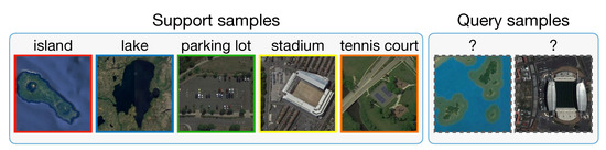
Figure 1.
Illustration of using few-shot learning to learn information from just one labeled image.
By seeing the potential that few-shot learning can alleviate the data-gathering effort, improve computing efficiency, and bridge the gap between Artificial Intelligence and human-like learning, we introduce the few-shot paradigm to the aerial scene classification problem. The goal of this work is to classify aerial scene images with only 1 or 5 labeled samples. More specifically, we adopt a meta-learning framework to address this problem. To the best of our knowledge, only a few efforts have focused on the few-shot classification problem in the aerial/remote scene regime. A deep few-shot learning method is proposed in work [26] to tackle the small sample size problem of hyperspectral image classification. The very recent work [33] developed a few-shot learning method based on Prototypical networks [32] for the classification of RS scene. By far, we are the first to provide a testbed for few-shot classification of aerial scene images. We re-implement several state-of-the-art few-shot learning approaches (i.e., Prototypical Networks [32], MAML [34] and Relation Network [35]) with a deeper backbone Resnet-12 for a fair comparison. In addition, we re-implement a typical machine learning classification method D-CNN [16], to evaluate its performance in the few-shot scenario.
The main contributions of this article are summarized as follows.
- This is the first work to provide a unified testbed for fair comparison with several state-of-the-art few-shot learning approaches in the aerial scene field. Our experimental evaluation reveals that it is possible to learn much information for a new category from just a few labeled images, which is a great potential for the remote sensing community.
- The proposed method including a feature extraction module and a meta-learning module. First, ResNet-12 is used as a backbone to learn a representation of input on base set. Then, in the meta-training stage, we optimize the classifier by cosine distance with a learnable scale parameter in the feature space, neither fix nor introduce any additional parameters. Our method is simple yet effective, achieves state-of-the-art performance on two challenging datasets: NWPU-RESISC45 and RSD46-WHU.
- We conduct extensive experiments and build a mini dataset from the RSD46-WHU to further investigate what factors aspect the performance, including the effect of dataset scale, the impact of different metrics and number of support shots. The experiment results demonstrate that our model is specifically effective in few-shot settings.
The remainder of this paper is organized as follows. In Section 2, we discuss the related work on CNN-based methods of aerial scene classification and various state-of-the-art few-shot classification approaches that developed recently. In Section 3, we introduce some preliminary of the few-shot classification as it may be new to some readers. The proposed meta-learning method is described in Section 4. We illustrate the datasets and discuss the experiment results in Section 5. Moreover, finally, Section 6 concludes the paper with a summary and an outlook.
2. Related Work
2.1. CNN-Based Methods of Aerial Scene Classification
Aerial scene classification has been well studied for the last few decades owing to its broad applications. Since the emergence of the AlexNet [22] in 2012, deep learning-based methods have made an enormous breakthrough, much defeated the traditional methods based on low-level and middle-level methods, and became mainstream in the aerial scene classification task.
One strand study attempted to use a transfer learning method to fine-tune the pre-trained CNNs for aerial image classification. In [17], Hu et al. studied how to transfer the activations of CNNs pre-trained on the ImageNet dataset to high-resolution remote sensing classification. Cheng et al. [18] obtained better performance by using fine-tuned AlexNet [22], VGGNet-16 [23], and GoogleNet [36] on the dataset NWPU-RESISC45. Similarly, Nogueira et al. [24] carried out three strategies, namely full training, fine-tuning, and using CNNs as feature extractors, for exploiting six common CNNs in three remote sensing datasets. Their experiment results demonstrate that fine-tuning is generally the best strategy in different situations.
Some further studies utilize the pre-trained CNNs for feature extraction and combine the high-level semantic features with hand-crafted features. Zhao and Du [37] proposed a CNN framework to learn local spatial patterns from multi-scale. Wang et al. [38] presented an encoded mixed-resolution representation framework where multilayer features are extracted from various convolutional layers. The study by Lu et al. [39] introduced an adaptive feature strategy that fuses the deep learning feature and the SIFT feature to overwhelm the scale and rotation variability, which is essential in remote sensing images but cannot be captured by CNN-based methods.
More recent research has begun to concern the problem of within-class diversity and between-class similarity in aerial scene images. For example, to tackle this issue, Cheng et al. [16] trained a discriminative CNN model by optimizing a novel objective function. Beyond a traditional cross-entropy loss, a metric learning regularization term and a weight decay term are added to the proposed objective function. Li et al. [25] constructed a feature fusion network that combining the original feature and attention map feature; besides that, they adopted center loss [40] to improve feature distinguishability.
2.2. Few-Shot Classification via Meta-Learning
Deep learning-based approaches have achieved remarkable success in various fields, especially in areas where vast quantities of data can be collected and where substantial computing resources are available. However, deep learning is often suffered from poor sample efficiency. Recently, few-shot learning is proposed to tackle this problem and have been marked by exceptional progress. Few-shot learning aims to learn new concepts from only small amounts of samples and quickly adapt to unforeseen tasks, which can be viewed as a special case of meta-learning. In the following, we introduce some representative few-shot classification literature, gathering into two main streams: optimization-based methods and metric-based methods.
Optimization-based methods. This line of work is most understood as learning to learn, which tackles the few-shot classification problem by effectively optimizing model parameters to new tasks. Finn et al. proposed a model-agnostic algorithm named MAML [34], which targets to learn a good initialization of any standard neural network. In such a way, it means to prepare that network for fast adaptation to any novel task through only one or a few gradient steps. The authors also presented a first-order approximation version of MAML by ignoring second-order derivatives to speed-up the network computation. Reptile [41] expands on the results from MAML by performing a Taylor series expansion update and finding a point near all solution manifolds of the training tasks. Many variants [42,43,44] of MAML follow a similar idea that, with a good initialization, one is just a few gradient steps away from a solution to a new task. These approaches face a critical challenge that the external optimization needs to solve as many parameters as internal optimization. Besides, there is a key debate. That is, whether a single initial condition is sufficient to provide fast adaption for a wide range of potential tasks. And further, whether an initial condition is restricted to relatively narrow distributions.
Metric-based methods. Another family of approach aims to address few-shot classification by learning to compare. The key insight of the idea is to learn a feature extractor that mapping raw input into a representation suitable for predicting, such that, when represented in this feature space, the query and support samples are easy for comparison (e.g., with Euclidean distance or cosine similarity). Matching Networks [45] mapping the support set via an attention mechanism to a function and then classifying the query sample by a weighted nearest-neighbor classifier in an embedding space. Prototypical Networks [32] follows a similar idea that learns a metric-based prediction rule over embeddings. The prototype of each category is represented by the mean embedding of samples, such that the classification can be performed by computing distances to the nearest category mean. Besides a usual embedding module, Relation Network [35] introduces an additional parameterized CNN-based ’relation module’ for learnable metric comparison. TADAM [46] presents an inspiring ProtoNet-based architecture that incorporates several useful modifications for few-shot learning, including metric scaling, task-conditioning, auxiliary task co-training. Ref. [47] extends the Prototypical Networks to a semi-supervised setting by adding unlabeled samples into each episode. Three strategies are explored to refine the samples’ mean location of the corresponding category. MetaOptNet [48] suggests that discriminatively trained linear classifiers (e.g., SVM or linear regression) may offer better performance than nearest neighbor classifiers in few-shot regimes. The linear classifiers can learn better class boundaries using negative examples at a modest increase in computational costs. Simon et al. [49] observed that high-order information is preferred over low-order to improve the classifier’s capability in the low data regime; hence one hopes a subspace method can form a robust classifier. The authors develop a dynamic classifier that computes a subspace of feature space for each category, and the features of query samples are projected into the subspace for comparison.
While meta-learning approaches have seen great success in few-show classification, some pre-trained methods have recently gained competitive performance [50,51]. Our work is more related to the second line of work by finding a suitable distance metric and taking the pre-trained method’s strength by learning good feature embeddings. A summary of the few-shot classification methods mentioned in this section is listed in Table A2 (Appendix A).
3. Preliminary
Before introducing our overall framework in detail, we first look at some preliminary of the few-shot classification as it may be new to some readers.
In standard supervised classification, we are dealing with a dataset . The training set takes labeled pairs as inputs, denoted as , , where N is the number of training samples, is the number of categories in . We are interested in learning a model , parameterized by on , to predict the label for an unlabeled sample on the test set .
In few-shot classification, we instead consider a meta-set and are chosen to be mutually disjoint, where represents the category. The vision is to learn a model on that can quickly adapt to unseen categories in with only a few support samples, usually 1 or 5. is held-out for choosing the hyperparameters and select the best model.
Following the standard FSL protocol [45,52], a model is often evaluated on a set of N-way K-shot classification tasks, denoted as , also known as episodes. To be specific, each episode has a split of support-set and query-set . The support-set contains N unique categories with K labeled samples in each, meaning that consists of samples for training. The query-set holds the same N categories, each with Q unlabeled samples being to classify. An episode is often constructed in the same way in training and testing. In other words, if we are supposed to perform 5-way 1-shot classification at test-time, then training episodes could be comprised of N = 5, K = 1. Figure 2 shows a visualization of 5-way 1-shot episodes. Note that, an entire task/episode in FSL is treated as a training instance in conventional machine learning.
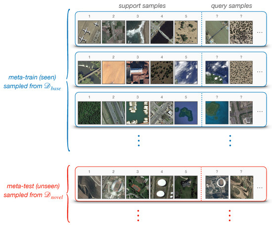
Figure 2.
Example: 5-way 1-shot classification episodes. The top represents the meta-training set of many tasks/episodes; each blue box is an episode that contains support samples and query samples. In this case, N = 5, K = 1, Q is usually 15. The meta-test set is defined in the same way, as shown at the bottom.
4. Proposed Method
4.1. Overall Framework
In this work, we propose a meta-learning method for few-shot classification of aerial scene images. The framework consists of a feature extractor, a meta-training stage, and a meta-testing stage. Figure 3 illustrates the overall procedure of our method. First, a feature extractor is trained on base dataset to learn a representation of inputs for further comparison in feature space. To achieve this, we train a typical classifier on all base categories by minimizing a standard cross-entropy loss and removing its last fully-connected (FC) Layer to get a 512-dimensional feature representation . Then, we consider training a meta-learning classifier over a set of episodes in the meta-training stage. Concretely, unlike some prior works [50,51], we do not freeze for further fine-tuning; instead, we treat it as an initial weight and optimize it directly by minimizing the generalization error across episodes. For a single episode, the query features are compared with the category mean of support features by scaled cosine distance. The goal of meta-training is to minimize the N-way prediction loss in the query set. Finally, in the meat-testing stage, the meta-learning classifier is estimated on a set of episodes sampled from the novel set , usually referred to as a meta-test set.
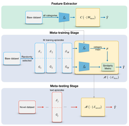
Figure 3.
Overall framework of our method. The top represents the feature extractor trained on the base dataset; by removing the FC layer, the network generates a feature encoder . The meta-training procedure aims to learn a meta classifier by optimizing the parameter from multiple episodes. In the meta-testing stage, the performance of the meta-classifier is evaluated once a new episodes sampled from unseen categories is provided.
4.2. Feature Extractor
We train a feature extractor with parameters on the base set that encodes the input data to a 512-dimensional feature vector suitable for comparison. Here we employ ResNet-12 to learn a classifier on all base categories and remove the last fully connected layer to get , which is described below; though, other backbones can also be used. Before feeding to the network, all input images in are resized to . The architectural setting of ResNet-12 we use, illustrated in Figure 4, consists of four ResNet blocks. Three convolutional layers configure each ResNet block with a kernel, followed by BN and Leaky ReLU. As shown in the figure below, denotes the channels of convolutional layers in each ResNet block, which is 64, 128, 256, 512, respectively. We then adopt a Leaky ReLU and max pooling layer right after each residual block. Lastly, by feeding the vector generated by the ResNet Block-4 to the average pooling layer, we can finally get a 512-dimensional feature representation, as mentioned in the beginning.
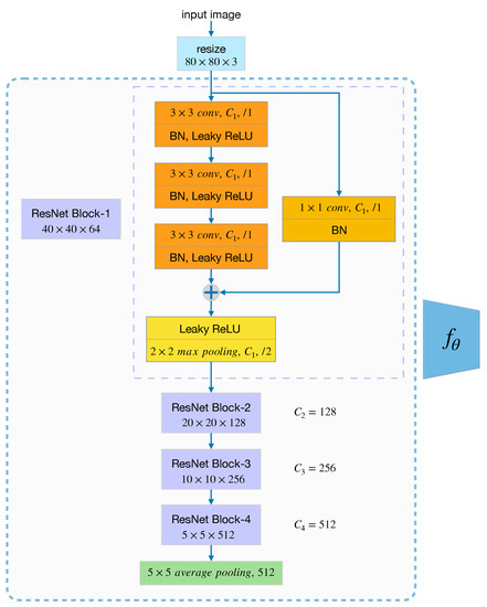
Figure 4.
The structure of ResNet-12 with four ResNet blocks.
4.3. Meta-Training Stage
Meta-learning aims to improve performance by extracting meta-knowledge from a set of tasks, aslo called episodes, which has been widely used in the few-shot classification problems. According to the conventional N-way K-shot setting, our goal is to train a meta-learning model that minimizes the N-way prediction loss. To accomplish this, we sample many episodes from training data in base categories. An episode has K input-output pairs randomly selected from each category, namely a total of samples for N-way classification training and query samples for test. Although only a limited number of support samples per episode are used for training, the parameters of classifier are shared across many episodes. Thus learning such from a large number of tasks reduces the sample requirement burden. During meta-training stage, an additional meta-validation set is held out to choose the hyper-parameters of the model . Figure 5 illustrates the workflow of the proposed meta-learning stage.
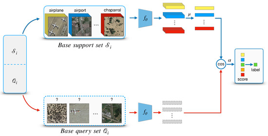
Figure 5.
The architecture of meta-training stage for a N-way K-shot classification problem.
Given an episode with the support-set , we denote as a subset of with all samples in category c [32] defined a prototype as the mean vector over embeddings belonging to (the centroid of category c), an embedding is generate by the pre-trained feature extractor with learnable parameters we described in Section 4.2. We can write down the as follows:
One intuitive way to predict the probability that a query sample x belongs to category c is to compare the distance between the feature embedding and the centroid of category c. Two common distance metrics are Euclidean distance and cosine similarity, here we employ the cosine similarity, and thus the prediction can be formalized as follows:
where denotes the cosine similarity of two vectors.
Inspired by the work [46], we introduce a learnable scalar parameter to adjust the original value range of cosine similarity. In our experiments, is initialized to 10, and we observe that the scaling similarity metric is more appropriate for the following softmax layer. Then, the predictive probability becomes:
4.4. Meta-Testing Stage
Once the meta-learning model is learned, its generalization is evaluated on a held-out set . Note that, all categories in novel-set are unseen in the meta-training stage. At meta-test time, we are given new episodes sampled from , often referred to as a meta-test set . The learned model is adapted to predict unseen categories with the new support set .
5. Experiments and Analysis
In this section, we first present some implementation details and dataset description. Then, we compare our method with three state-of-the-art few-shot methods and one typical CNN-based method, D-CNN. In addition, we conduct a new dataset mini-RSD46-WHU to investigate how the scale of the dataset impacts the results. At last, we also carry out experiments to evaluate the 5-way accuracy as a function of shots.
5.1. Implementation Details
Following the few-shot experimental protocol proposed by Vinyals, O. [45], we carry out the experiments of N-way classification with K shots, here N = 5, K = 1 or 5. In the meta-training procedure, a few-shot training batch is composed of several episodes where an episode is a selection of 5 randomly categories drawn from . We set 4 episodes per batch to compute the average loss, namely the batch size is 4, the amount depends on the size of the GPU memory. The support set in each training episode are expected to match the same number of shots as in the meta-test stage. That is, for example, if we want to perform 5-way 1-shot classification at test-time, then the training episodes could be constituted of N = 5, K = 1. Note that each category contains K query samples during meta-training stage and 15 query samples during meta-testing.
In traditional deep learning, an epoch is an entire dataset passes forward and backward through the neural network once. In few-shot learning, we sample episodes randomly from the dataset. Although there are only limited training samples in each episode, when the number of episodes is large enough(e.g., in our work, an epoch contains 1000 episodes), one can assume that the entire dataset has been probably traversed.
We employ Resnet-12 as our backbone; by removing the fully connected layer, the network generates a 512-dimensional feature vector for each input image. For this step, we use SGD optimizer with momentum 0.9, the learning rate is initialized to 0.1, and the decay factor is set to 0.1. The feature extractor was trained for 100 epochs with batch size 128 on 4 GPUs, the weight decay for ResNet-12 is 0.0005. For ProtoNet [32], MAML [34], and RelationNet [35], we first follow the original literature and adopt a four-layer convolutional backbone (Conv-4). For a better comparison, we we re-implement these three methods with ResNet-12 backbone to investigate if a deeper backbone benefits the performance. In addition, we re-implement a typical machine learning classification method D-CNN [16], to evaluate its performance in the few-shot scenario. ResNet-12 and the same settings are used in the D-CNN re-implementation. All our code was implemented in Pytorch and run with 4 NVIDIA RTX 2080 Ti. Note that, training in DSN-MR [49] with a ResNet-12 backbone requires 4 GPUs with ∼10 GB/GPU.
5.2. Datasets Description
We evaluate our proposed method on two challenging datasets: NWPU-RESISC45 [18] and RSD46-WHU [30,31]. Besides, to answer the question of how the dataset scale impacts the performance, we construct a mini dataset from the RSD46-WHU dataset. The details of the considered datasets are described as follows:
The NWPU-RESISC45 dataset was proposed by Cheng et al. [18] in 2017 and became a popular benchmark in the RS classification research. It involves 45 categories with 700 remote scene images in each category, each with a size of pixels. These aerial images are collected by experienced experts from Google Earth; the spatial resolution ranges from approximately 30 to 0.2 m per pixel. According to the split division setting proposed by Ravi et al. [52], we split the 45 categories into 25, 8, 12 for meta-training, meta-validation and meta-testing, respectively. Note that, the validation set was held-out for hyper-parameter selection of the meta-training stage. The set split for meta-training are the same 25 categories of . It is further divided into three sets: meta-train-support, meta-train-val, meta-train-query. The number of images in each category is shown in Table 1.

Table 1.
NWPU-RESISC45 Dataset split.
The RSD46-WHU dataset contains 46 categories, each with images ranging from 428 to 3000, for a total of 117,000. Like many other RS datasets, the images are collected by hand from Google Earth and Tianditu, with the ground resolution spanning from 0.5 m to 2 m. Similar to the NWPU-RESISC45 dataset, that the 46 categories in RSD46-WHU dataset are divided into 26, 8, 12 for meta-training, meta-validation, and meta-testing, respectively. It is relevant to mention that we have dropped about 1200 images in total because some images are not in the size of pixels or contain incorrect content. The details of our modified dataset-split are listed in Table 2.
Table 2.
RSD46-WHU Dataset split.
We further conduct a new dataset mini-RSD46-WHU to investigate how the scale of the dataset impacts the results. The mini-RSD46-WHU dataset is formed from the RSD46-WHU dataset by randomly selecting 500 images in each category. Except for category Sewage plant-type-two only has 428 images, because that is all it holds in the original dataset. We follow the same division setting of the RSD46-WHU dataset; the only change is the number of images in each category. Table 3 shows the details.
Table 3.
mini-RSD46-WHU Dataset split.
5.3. Results and Comparisons
Following the most common setting in few-shot classification, namely 5-way 1-shot, and 5-way 5-shot, we conduct experiments to evaluate the effectiveness of our method. The proposed method is compared with various state-of-the-art few-shot learning methods and one conventional deep learning method.
For 5-way 1-shot experiment, one labeled support sample per category is randomly selected as the supervised sample at the test time. Likewise, 5 support samples per category are provided for 5-shot setting. Following the evaluation protocols of FSL [32,52], 15 query images per category are batched in each episode for evaluation. We computed the mean classification accuracy of 2000 randomly generated episodes from the novel (meta-test) set.
We note that the original backbone of Prototypical Networks (ProtoNet) [32], MAML [34], and RelationNet [35] is Conv-4, while a deeper backbone like Resnet-12 used in others may benefit the performance. Thus, we re-implement these three methods with ResNet-12 backbone for a fair comparison. Also, the performance of a conventional classification algorithm D-CNN [16] is analyzed in few-shot classification scenarios.
On both datasets, the results of average 5-way accuracy (%) with 95% confidence interval of 1-shot and 5-shot are reported in Table 4 and Table 5 respectively. The symbol * indicates our re-implementation of ProtoNet, MAML, and RelationNet with ResNet-12 backbone. As we can see, our method outperforms the other models under both 5-way 1-shot and 5-way 5-shot settings. D-CNN shows inferior performance both in the 1-shot and 5-shot cases, and this result is reasonable due to D-CNN is not designed specifically to few-shot classification. Typical CNNs-based methods most likely lead to overfitting when meeting so few supervised samples, whereas meta-based methods have achieved considerable performance.
Table 4.
Few-shot classification results on NWPU-RESISC45. The symbol * indicates our re-implementation of ProtoNet, MAML, and RelationNet with ResNet-12 backbone. Marked in bold are the best results for each scenario.
Table 5.
Few-shot classification results on RSD46-WHU. The symbol * indicates our re-implementation of ProtoNet, MAML, and RelationNet with ResNet-12 backbone. Marked in bold are the best results for each scenario.
A bar chart of few-shot classification results on both datasets are shown in Figure 6 and Figure 7. We observe that our method gets the best performance among all popular methods despite its simple design.
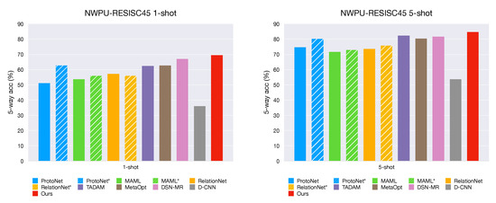
Figure 6.
Few-shot classification results on the NWPU-RESISC45 dataset. The striped bars indicate the approaches in our re-implementation with Resnet-12 backbone. The performance is reported with 95% confidence intervals.
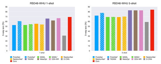
Figure 7.
Few-shot classification results on the RSD46-WHU dataset. The striped bars indicate the approaches in our re-implementation with Resnet-12 backbone. The performance is reported with 95% confidence intervals.
For MAML, a representative method for model initialization, we adopt a first-order approximation version for the experiments. The original paper of MAML reports that the performance of the first-order approximation is almost identical to the full version. We take the first-order approximation version for its efficiency; the performance of MAML may get narrowly enhance by the full version. Similar to our method, ProtoNet and RelationNet are both metric-based methods. ProtoNet uses Euclidean distance while RelationNet compares an embedding and query samples using an additional parameterized CNN-based ’relation module’. MetaOptNet [48] and DSN-MR [49] are also metric-based approaches. MetaOptNet provides an end-to-end method with regularized linear classifiers i.e., ridge regression and SVM. On the other hand, DSN-MR provides another enlightening perspective: a subspace of the feature space is computed for each category, and then the query sample is projected into the subspace, where the distance measurement is performed. Our method computes the class centers as the same in ProtoNet, yet we employ a cosine distance with a learnable scaling factor for classifying which contributes a lot to achieve better performance. We conduct an ablation experiment to investigate the impact of metric in Section 5.4. TADAM [46] assumes a task-conditioned feature extractor should be more discriminative for a given task. They presented a dynamic feature extractor that can be optimized by a given support set . However, this strategy introduces additional complexity to the architecture; they solve this problem by adopting an additional logit head (i.e., the normal M-way classification, where M is the number of all categories in the base set) for auxiliary co-training. We take a different strategy that trains a normal M-way classification on the seen categories(base-set) but does not introduce any additional parameters. Instead, we remove the last FC layer to get an encoder , whose weights are then used as initialization. It gives a good boost in the meta-training stage for further optimization.
As shown in Figure 6 and Figure 7, the striped bars indicate our re-implementation of MAML, ProtoNet, and RelationNet with ResNet-12 backbone. We observed that a deeper backbone (Resnet-12) slightly improves MAML and RelationNet; moreover, RelationNet even gets worse in the 1-shot case for both datasets. On the other hand, the Prototypical Network (ProtoNet) is improved by a large margin when the backbone architecture is replaced with Resnet-12, which shows that ProtoNet is a powerful and robust approach.
An interesting phenomenon we observed is shown in Figure 8. We plot the first 90 epochs of the generalization of our model on base and novel categories. Base generalization indicates the training accuracy from unseen data in the base categories, and the novel generalization means test performance from data in novel categories. As shown, while the model achieves better performance on unseen data in the base set, the novel generalization drops instead. Why the test performance decreases? We suppose lacking supervised data is the reason causing the over-fitting problem, which leads to this phenomenon. This problem will be discussed further in Section 5.4.
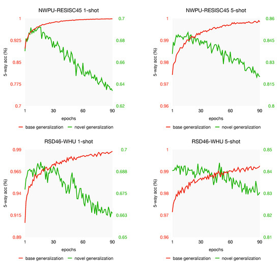
Figure 8.
Generalization discrepancy in meta-learning stage.
5.4. Analysis
5.4.1. Effect of Dataset Scale
To investigate how dataset scale impacts the performance, we conduct a variant of the RSD46-WHU dataset with only 500 images in each category, called mini-RSD46-WHU. The overall accuracies of 5-way 1-shot and 5-shot are reported in Table 6. We adopt the same backbone and training strategy on both datasets. As we can see, apparently, the performance improves when the scale of dataset gets larger. The overall accuracy of 5-way 1-shot and 5-shot on the original dataset increased by 6.86% and 5.78% compared to the mini dataset.
Table 6.
Comparison between mini and full RSD46-WHU.
5.4.2. Effect of Metrics
We investigate the impact of different metric strategies for the few-shot classification, i.e., based on the Euclidean distance and cosine similarity. The two choices are compared in Table 7; furthermore, we study the effect of scaling parameter by adding it to both metrics. The scaling parameter is empirically initialized as 0.1 for Euclidean distance and 10 for cosine similarity. As shown in Tabe Table 7, the performance improves to 69.02 ± 0.22% and 68.56 ± 0.25%, respectively, in the 5-way 1-shot case. This shows a gain of 8.61% and 8.87% with a simple cosine similarity instead of Euclidean distance. In the case of 5-shot, the improvement is slight, 0.69% and 0.74%, respectively. Further, we can see that, for both datasets in 1-shot and 5-shot case, the scale parameter gives about ∼0.3% to ∼0.5% gain compared with using cosine similarity only. However, the scale parameter has barely improved or gotten worse for the performance of Euclidean distance.
Table 7.
The effect of different metrics on test performance with 95% confidence intervals when training on NWPU-RESISC45 and RSD46-WHU. Marked in bold are the best results for each scenario.
5.4.3. Effect of Shots
To further evaluate the 5-way accuracy as a function of shots, we conduct the experiments by providing our model with 1, 5, 10, 15, 20, and 25 labeled support samples on both datasets. The results are presented in Figure 9. As we expected, the prediction accuracy is greatly improved when the shot is increasing from 1 to 5. However, the performance does not benefit much more when the shot continues to increase. These findings confirm that our model is specifically effective in very-low-shot settings.
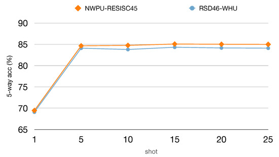
Figure 9.
The effect of shots on test performance are reported with 95% confidence intervals when training on NWPU-RESISC45 and RSD46-WHU. All experiments are from 5-way classification with a ResNet-12 backbone.
From the experiments in Section 5.3, we observe from Figure 8 that the model with the best accuracy often appears in the first 40 epochs. For a further analysis of the generalization discrepancy, we plot the generalization curve with different shots on both NWPU-RESISC45 and RSD46-WHU datasets, see Figure 10 and Figure 11. As we can see, the same phenomenon appeared again: when the generalization gets better on the unseen data of base, indicating that the model learns the objective better, whereas the test performance gets worse on the novel task. In other words, this phenomenon still exists when the support labeled instances increases; over-fitting may not be the very reason for the test performance drops. This generalization discrepancy may be caused by the objective difference between the novel set and the base set. That is, in the meta-training stage, our model learns too specific on base-set, which has adverse effects on the novel-set. Our investigations suggest that the generalization discrepancy might be a potential challenge in few-shot learning. Some careful regularization terms might be helpful to narrow the gap of generalization discrepancy, which we leave for future work.
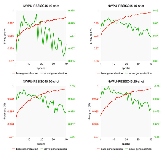
Figure 10.
The effect of shots on test performance are reported with 95% confidence intervals when training on NWPU-RESISC45 and RSD46-WHU. All experiments are from 5-way classification with a ResNet-12 backbone.
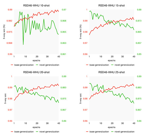
Figure 11.
The effect of shots on test performance are reported with 95% confidence intervals when training on NWPU-RESISC45 and RSD46-WHU. All experiments are from 5-way classification with a ResNet-12 backbone.
6. Conclusions
The topic of few-shot learning has attracted much attention in recent years. In this paper, we bring few-shot learning to aerial scene classification and demonstrate that useful information may be learned from a few instances. To pursue this idea, we proposed a meta-learning framework which aims to train a model that generalizes well on unseen categories when providing a few samples. The proposed method first employs ResNet-12 to learn a representation on base-set, and then in the meta-training stage, we optimize the classifier by cosine distance with a learnable scale parameter. Our experiments, conducted on two challenging datasets, are encouraging in that our method can achieve a classification performance of around 69% for a new category by just providing one instance, besides approximately 84% for 5 support samples. Furthermore, we have conducted several ablation experiments to investigate the effects of dataset scale, the impact of different metrics and the number of support shots. At last, we observe an interesting phenomenon that there is potentially a generalization discrepancy in meta-learning. We suggest that further research in this phenomenon may be an opportunity to achieve better performance in the future.
Author Contributions
Conceptualization, P.Z., Y.B., D.W. and Y.L.; Data curation, P.Z., Y.B. and D.W.; Investigation, P.Z., Y.B. and D.W.; Methodology, P.Z., D.W. and Y.L.; Validation, P.Z., Y.B., D.W. and B.B.; visualization, P.Z.; Writing—original draft, P.Z.; Writing—review & editing, P.Z. and Y.L.; supervision, B.B. and Y.L. All authors have read and agreed to the published version of the manuscript.
Funding
This work was supported in part by the National Natural Science Foundation of China under Grant 61871460; in part by the Shaanxi Provincial Key Research and Development Program under Grant 2020KW-003; in part by the Fundamental Research Funds for the Central Universities under Grant 3102019ghxm016.
Acknowledgments
We would like to express our gratitude to the editor and reviewers for their valuable comments.
Conflicts of Interest
The authors declare no competing financial interests. The founding sponsors had no role in the design of the study; in the collection, analyses, or interpretation of data; in the writing of the manuscript; and in the decision to publish the results.
Appendix A
Table A1.
Comparison of the six common aerial datasets.
Table A1.
Comparison of the six common aerial datasets.
| Dataset | # Categories | Images per Category | Total Images | Image Sizes | Year |
|---|---|---|---|---|---|
| UC Merced dataset [12] | 21 | 100 | 2100 | 256 × 256 | 2010 |
| WHU-RS19 [28] | 19 | 50 | 950 | 600 × 600 | 2010 |
| AID dataset [7] | 30 | 220–420 | 10,000 | 600 × 600 | 2016 |
| NWPU-RESISC45 [18] | 45 | 700 | 31,500 | 256 × 256 | 2016 |
| RSD46-WHU [30,31] | 46 | 500–3000 | 117,000 | 256 × 256 | 2016 |
| PatternNet dataset [29] | 38 | 800 | 30,400 | 256 × 256 | 2017 |
Table A2.
Characteristics of few-shot learning methods. a-b-c-d denotes a 4-layer convolutional network with a, b, c, and d filters in each layer.
Table A2.
Characteristics of few-shot learning methods. a-b-c-d denotes a 4-layer convolutional network with a, b, c, and d filters in each layer.
| Methods | Backbone | Year | Characteristics | |
|---|---|---|---|---|
| Optimization-based | MAML [34] | 32-32-32-32 | 2017 | model-agnostic, learn a good initialization for fast-adapting to new tasks |
| Reptile [41] | 32-32-32-32 | 2018 | first-order approximation of MAML | |
| LEO [42] | WRN-28-10 | 2019 | introduce low-dimensional latent space to MAML | |
| MTL [43] | ResNet-12 | 2019 | learn Scaling and Shifting parameters by adopting hard task training strategy | |
| Metric-based | MathingNets [45] | 64-64-64-64 | 2016 | cosine similarity |
| ProtoNet [32] | 64-64-64-64 | 2017 | Euclidean distance | |
| RelationNet [35] | 64-96-128-256 | 2018 | additional CNN relation module | |
| TADAM [46] | ResNet-12 | 2018 | scaled Euclidean distance, task-specific | |
| MetaOptNet [48] | ResNet-12 | 2019 | ridge regression, SVM | |
| DSN-MR [49] | ResNet-12 | 2020 | subspace, SVD |
References
- Hu, Q.; Wu, W.; Xia, T.; Yu, Q.; Yang, P.; Li, Z.; Song, Q. Exploring the Use of Google Earth Imagery and Object-Based Methods in Land Use/Cover Mapping. Remote Sens. 2013, 5, 6026–6042. [Google Scholar] [CrossRef]
- Pham, H.M.; Yamaguchi, Y.; Bui, T.Q. A case study on the relation between city planning and urban growth using remote sensing and spatial metrics. Landsc. Urban Plan. 2011, 100, 223–230. [Google Scholar] [CrossRef]
- Cheng, G.; Guo, L.; Zhao, T.; Han, J.; Li, H.; Fang, J. Automatic landslide detection from remote-sensing imagery using a scene classification method based on BoVW and pLSA. Int. J. Remote Sens. 2013, 34, 45–59. [Google Scholar] [CrossRef]
- Zhu, Q.; Zhong, Y.; Zhao, B.; Xia, G.S.; Zhang, L. Bag-of-visual-words scene classifier with local and global features for high spatial resolution remote sensing imagery. IEEE Geosci. Remote Sens. Lett. 2016, 13, 747–751. [Google Scholar] [CrossRef]
- Li, X.; Shao, G. Object-based urban vegetation mapping with high-resolution aerial photography as a single data source. Int. J. Remote Sens. 2013, 34, 771–789. [Google Scholar] [CrossRef]
- Manfreda, S.; McCabe, M.F.; Miller, P.E.; Lucas, R.; Pajuelo Madrigal, V.; Mallinis, G.; Ben Dor, E.; Helman, D.; Estes, L.; Ciraolo, G. On the use of unmanned aerial systems for environmental monitoring. Remote Sens. 2018, 10, 641. [Google Scholar] [CrossRef]
- Xia, G.S.; Hu, J.; Hu, F.; Shi, B.; Bai, X.; Zhong, Y.; Zhang, L.; Lu, X. AID: A benchmark data set for performance evaluation of aerial scene classification. IEEE Trans. Geosci. Remote Sens. 2017, 55, 3965–3981. [Google Scholar] [CrossRef]
- Swain, M.J.; Ballard, D.H. Color indexing. Int. J. Comput. Vis. 1991, 7, 11–32. [Google Scholar] [CrossRef]
- Manjunath, B.S.; Ma, W.Y. Texture features for browsing and retrieval of image data. IEEE Trans. Pattern Anal. Mach. Intell. 1996, 18, 837–842. [Google Scholar] [CrossRef]
- Lowe, D.G. Distinctive image features from scale-invariant keypoints. Int. J. Comput. Vis. 2004, 60, 91–110. [Google Scholar] [CrossRef]
- Ojala, T.; Pietikainen, M.; Maenpaa, T. Multiresolution gray-scale and rotation invariant texture classification with local binary patterns. IEEE Trans. Pattern Anal. Mach. Intell. 2002, 24, 971–987. [Google Scholar] [CrossRef]
- Yang, Y.; Newsam, S. Bag-of-visual-words and spatial extensions for land-use classification. In Proceedings of the 18th SIGSPATIAL International Conference on Advances in Geographic Information Systems, San Jose, CA, USA, 2–5 November 2010; pp. 270–279. [Google Scholar]
- Lazebnik, S.; Schmid, C.; Ponce, J. Beyond bags of features: Spatial pyramid matching for recognizing natural scene categories. In Proceedings of the 2006 IEEE Computer Society Conference on Computer Vision and Pattern Recognition (CVPR’06), New York, NY, USA, 17–22 June 2006; Volume 2, pp. 2169–2178. [Google Scholar]
- Jegou, H.; Perronnin, F.; Douze, M.; Sánchez, J.; Perez, P.; Schmid, C. Aggregating local image descriptors into compact codes. IEEE Trans. Pattern Anal. Mach. Intell. 2011, 34, 1704–1716. [Google Scholar] [CrossRef]
- Bosch, A.; Zisserman, A.; Muñoz, X. Scene classification via pLSA. In Proceedings of the European Conference on Computer Vision, Graz, Austria, 7–13 May 2006; pp. 517–530. [Google Scholar]
- Cheng, G.; Yang, C.; Yao, X.; Guo, L.; Han, J. When deep learning meets metric learning: Remote sensing image scene classification via learning discriminative CNNs. IEEE Trans. Geosci. Remote Sens. 2018, 56, 2811–2821. [Google Scholar] [CrossRef]
- Hu, F.; Xia, G.S.; Hu, J.; Zhang, L. Transferring deep convolutional neural networks for the scene classification of high-resolution remote sensing imagery. Remote Sens. 2015, 7, 14680–14707. [Google Scholar] [CrossRef]
- Cheng, G.; Han, J.; Lu, X. Remote sensing image scene classification: Benchmark and state of the art. Proc. IEEE 2017, 105, 1865–1883. [Google Scholar] [CrossRef]
- Zou, Q.; Ni, L.; Zhang, T.; Wang, Q. Deep learning based feature selection for remote sensing scene classification. IEEE Geosci. Remote Sens. Lett. 2015, 12, 2321–2325. [Google Scholar] [CrossRef]
- Wang, J.; Yang, J.; Yu, K.; Lv, F.; Huang, T.; Gong, Y. Locality-constrained linear coding for image classification. In Proceedings of the 2010 IEEE Computer Society Conference on Computer Vision and Pattern Recognition, San Francisco, CA, USA, 13–18 June 2010; pp. 3360–3367. [Google Scholar]
- Blei, D.M.; Ng, A.Y.; Jordan, M.I. Latent dirichlet allocation. J. Mach. Learn. Res. 2003, 3, 993–1022. [Google Scholar]
- Krizhevsky, A.; Sutskever, I.; Hinton, G.E. Imagenet classification with deep convolutional neural networks. Adv. Neural Inf. Process. Syst. 2012, 25, 1097–1105. [Google Scholar] [CrossRef]
- Simonyan, K.; Zisserman, A. Very Deep Convolutional Networks for Large-Scale Image Recognition. In Proceedings of the International Conference on Learning Representations, San Diego, CA, USA, 7–9 May 2015. [Google Scholar]
- Nogueira, K.; Penatti, O.A.; Dos Santos, J.A. Towards better exploiting convolutional neural networks for remote sensing scene classification. Pattern Recognit. 2017, 61, 539–556. [Google Scholar] [CrossRef]
- Li, J.; Lin, D.; Wang, Y.; Xu, G.; Zhang, Y.; Ding, C.; Zhou, Y. Deep discriminative representation learning with attention map for scene classification. Remote Sens. 2020, 12, 1366. [Google Scholar] [CrossRef]
- Liu, B.; Yu, X.; Yu, A.; Zhang, P.; Wan, G.; Wang, R. Deep few-shot learning for hyperspectral image classification. IEEE Trans. Geosci. Remote Sens. 2018, 57, 2290–2304. [Google Scholar] [CrossRef]
- Marcus, G.F. Rethinking eliminative connectionism. Cogn. Psychol. 1998, 37, 243–282. [Google Scholar] [CrossRef]
- Xia, G.S.; Yang, W.; Delon, J.; Gousseau, Y.; Sun, H.; Maître, H. Structural High-resolution Satellite Image Indexing. In ISPRS TC VII Symposium—100 Years ISPRS; Székely, W., Ed.; 2010; Volume XXXVIII, pp. 298–303. Available online: https://hal.archives-ouvertes.fr/file/index/docid/467740/filename/structural_satellite_indexing_XYDG.pdf (accessed on 16 November 2020).
- Zhou, W.; Newsam, S.; Li, C.; Shao, Z. PatternNet: A benchmark dataset for performance evaluation of remote sensing image retrieval. ISPRS J. Photogramm. Remote Sens. 2018, 145, 197–209. [Google Scholar] [CrossRef]
- Long, Y.; Gong, Y.; Xiao, Z.; Liu, Q. Accurate object localization in remote sensing images based on convolutional neural networks. IEEE Trans. Geosci. Remote Sens. 2017, 55, 2486–2498. [Google Scholar] [CrossRef]
- Xiao, Z.; Long, Y.; Li, D.; Wei, C.; Tang, G.; Liu, J. High-resolution remote sensing image retrieval based on CNNs from a dimensional perspective. Remote Sens. 2017, 9, 725. [Google Scholar] [CrossRef]
- Snell, J.; Swersky, K.; Zemel, R. Prototypical networks for few-shot learning. Adv. Neural Inf. Process. Syst. 2017, 30, 4077–4087. [Google Scholar]
- Alajaji, D.; Alhichri, H.S.; Ammour, N.; Alajlan, N. Few-Shot Learning For Remote Sensing Scene Classification. In Proceedings of the 2020 Mediterranean and Middle-East Geoscience and Remote Sensing Symposium (M2GARSS), Tunis, Tunisia, 9–11 March 2020; pp. 81–84. [Google Scholar]
- Finn, C.; Abbeel, P.; Levine, S. Model-Agnostic Meta-Learning for Fast Adaptation of Deep Networks. In Proceedings of the 34th International Conference on Machine Learning (ICML’17), Sydney, Australia, 6–11 August 2017; Volume 70, pp. 1126–1135. [Google Scholar]
- Sung, F.; Yang, Y.; Zhang, L.; Xiang, T.; Torr, P.H.; Hospedales, T.M. Learning to compare: Relation network for few-shot learning. In Proceedings of the IEEE Conference on Computer Vision and Pattern Recognition, Salt Lake City, UT, USA, 18–22 June 2018; pp. 1199–1208. [Google Scholar]
- Szegedy, C.; Liu, W.; Jia, Y.; Sermanet, P.; Reed, S.; Anguelov, D.; Erhan, D.; Vanhoucke, V.; Rabinovich, A. Going deeper with convolutions. In Proceedings of the IEEE Conference on Computer Vision and Pattern Recognition, Boston, MA, USA, 7–12 June 2015; pp. 1–9. [Google Scholar]
- Zhao, W.; Du, S. Scene classification using multi-scale deeply described visual words. Int. J. Remote Sens. 2016, 37, 4119–4131. [Google Scholar] [CrossRef]
- Wang, G.; Fan, B.; Xiang, S.; Pan, C. Aggregating rich hierarchical features for scene classification in remote sensing imagery. IEEE J. Sel. Top. Appl. Earth Obs. Remote Sens. 2017, 10, 4104–4115. [Google Scholar] [CrossRef]
- Lu, X.; Ji, W.; Li, X.; Zheng, X. Bidirectional adaptive feature fusion for remote sensing scene classification. Neurocomputing 2019, 328, 135–146. [Google Scholar] [CrossRef]
- Wen, Y.; Zhang, K.; Li, Z.; Qiao, Y. A discriminative feature learning approach for deep face recognition. In Proceedings of the European Conference on Computer Vision, Amsterdam, The Netherlands, 11–14 October 2016; pp. 499–515. [Google Scholar]
- Nichol, A.; Achiam, J.; Schulman, J. On first-order meta-learning algorithms. arXiv 2018, arXiv:1803.02999. [Google Scholar]
- Rusu, A.A.; Rao, D.; Sygnowski, J.; Vinyals, O.; Pascanu, R.; Osindero, S.; Hadsell, R. Meta-Learning with Latent Embedding Optimization. In Proceedings of the International Conference on Learning Representations, New Orleans, LA, USA, 6–9 May 2019. [Google Scholar]
- Sun, Q.; Liu, Y.; Chua, T.S.; Schiele, B. Meta-transfer learning for few-shot learning. In Proceedings of the IEEE Conference on Computer Vision and Pattern Recognition, Long Beach, CA, USA, 16–20 June 2019; pp. 403–412. [Google Scholar]
- Jamal, M.A.; Qi, G.J. Task agnostic meta-learning for few-shot learning. In Proceedings of the IEEE Conference on Computer Vision and Pattern Recognition, Long Beach, CA, USA, 16–20 June 2019; pp. 11719–11727. [Google Scholar]
- Vinyals, O.; Blundell, C.; Lillicrap, T.; kavukcuoglu, K.; Wierstra, D. Matching Networks for One Shot Learning. In Advances in Neural Information Processing Systems 29; Lee, D.D., Sugiyama, M., Luxburg, U.V., Guyon, I., Garnett, R., Eds.; Curran Associates, Inc.: Red Hook, NY, USA, 2016; pp. 3630–3638. [Google Scholar]
- Oreshkin, B.; Rodríguez López, P.; Lacoste, A. TADAM: Task dependent adaptive metric for improved few-shot learning. In Advances in Neural Information Processing Systems 31; Curran Associates, Inc.: Red Hook, NY, USA, 2018; pp. 721–731. [Google Scholar]
- Ren, M.; Ravi, S.; Triantafillou, E.; Snell, J.; Swersky, K.; Tenenbaum, J.B.; Larochelle, H.; Zemel, R.S. Meta-Learning for Semi-Supervised Few-Shot Classification. In Proceedings of the International Conference on Learning Representations, Vancouver, BC, Canada, 30 April–3 May 2018. [Google Scholar]
- Lee, K.; Maji, S.; Ravichandran, A.; Soatto, S. Meta-learning with differentiable convex optimization. In Proceedings of the IEEE Conference on Computer Vision and Pattern Recognition, Long Beach, CA, USA, 16–20 June 2019; pp. 10657–10665. [Google Scholar]
- Simon, C.; Koniusz, P.; Nock, R.; Harandi, M. Adaptive Subspaces for Few-Shot Learning. In Proceedings of the IEEE/CVF Conference on Computer Vision and Pattern Recognition, Seattle, WA, USA, 14–19 June 2020; pp. 4136–4145. [Google Scholar]
- Chen, W.Y.; Liu, Y.C.; Kira, Z.; Wang, Y.C.; Huang, J.B. A Closer Look at Few-shot Classification. In Proceedings of the International Conference on Learning Representations, New Orleans, LA, USA, 6–9 May 2019. [Google Scholar]
- Dhillon, G.S.; Chaudhari, P.; Ravichandran, A.; Soatto, S. A Baseline for Few-Shot Image Classification. In Proceedings of the International Conference on Learning Representations, Addis Ababa, Ethiopia, 26–30 April 2020. [Google Scholar]
- Ravi, S.; Larochelle, H. Optimization as a Model for Few-Shot Learning. In Proceedings of the ICLR, Toulon, France, 24–26 April 2017. [Google Scholar]


Publisher’s Note: MDPI stays neutral with regard to jurisdictional claims in published maps and institutional affiliations. |
© 2020 by the authors. Licensee MDPI, Basel, Switzerland. This article is an open access article distributed under the terms and conditions of the Creative Commons Attribution (CC BY) license (http://creativecommons.org/licenses/by/4.0/).