Global 3D Features of Error Variances of GPS Radio Occultation and Radiosonde Observations


Abstract
:1. Introduction
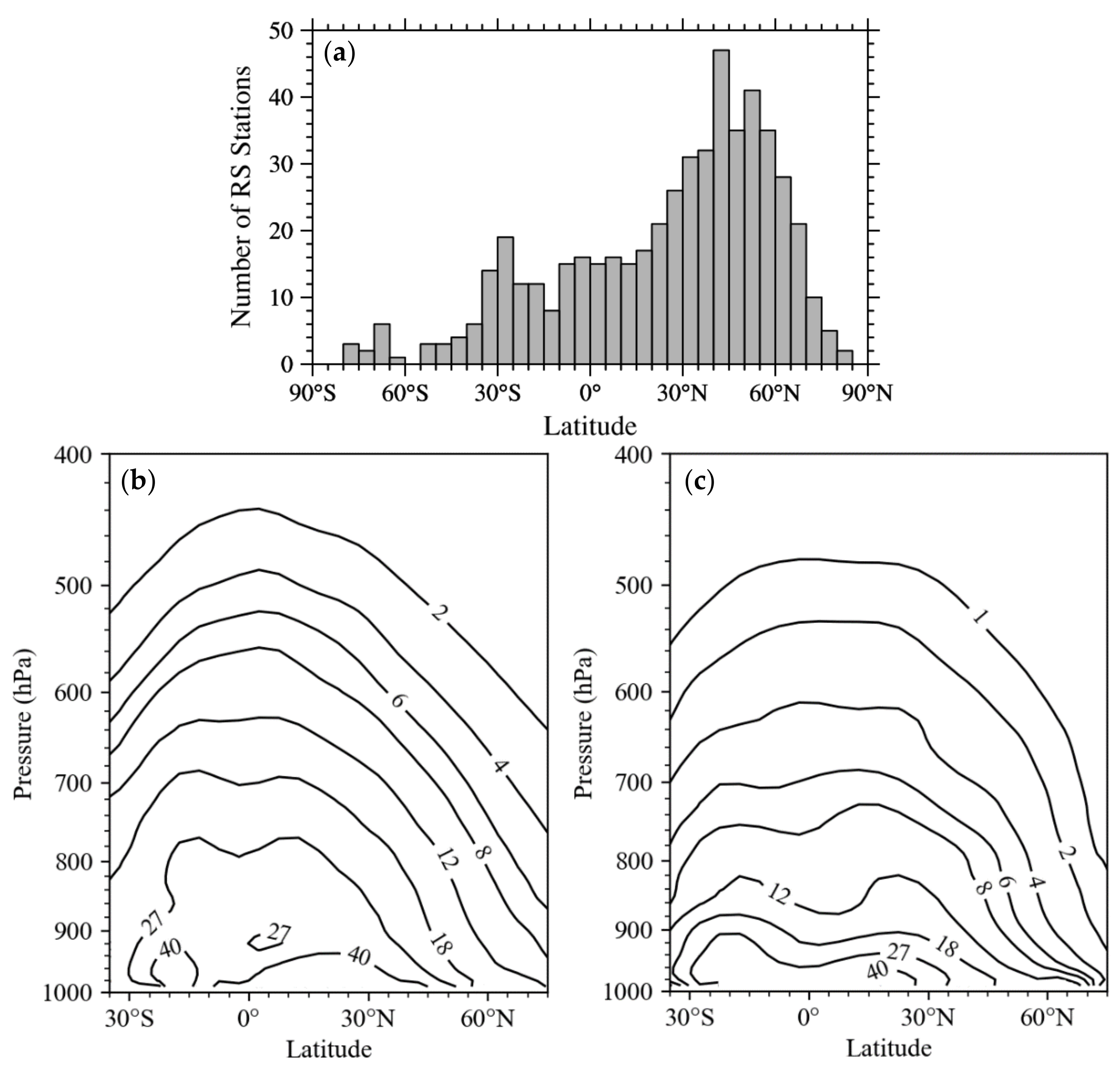
2. Data Description
3. Methodology
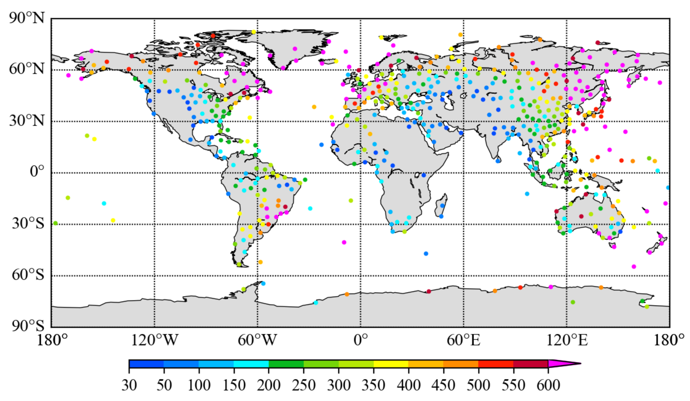
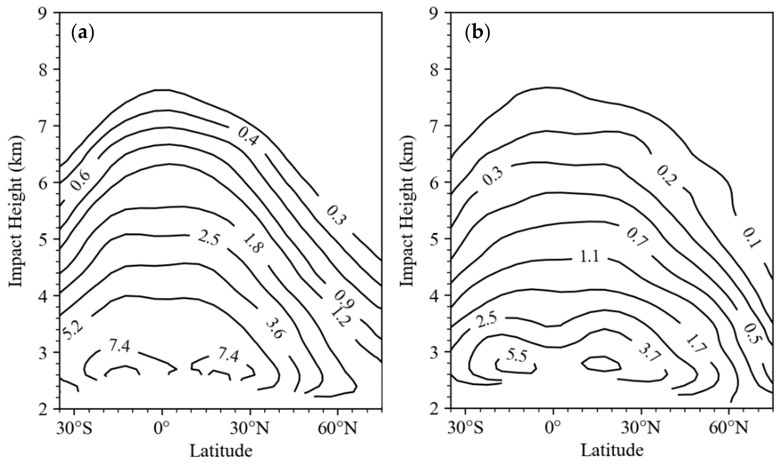
4. Global Error Variances of RO Observations
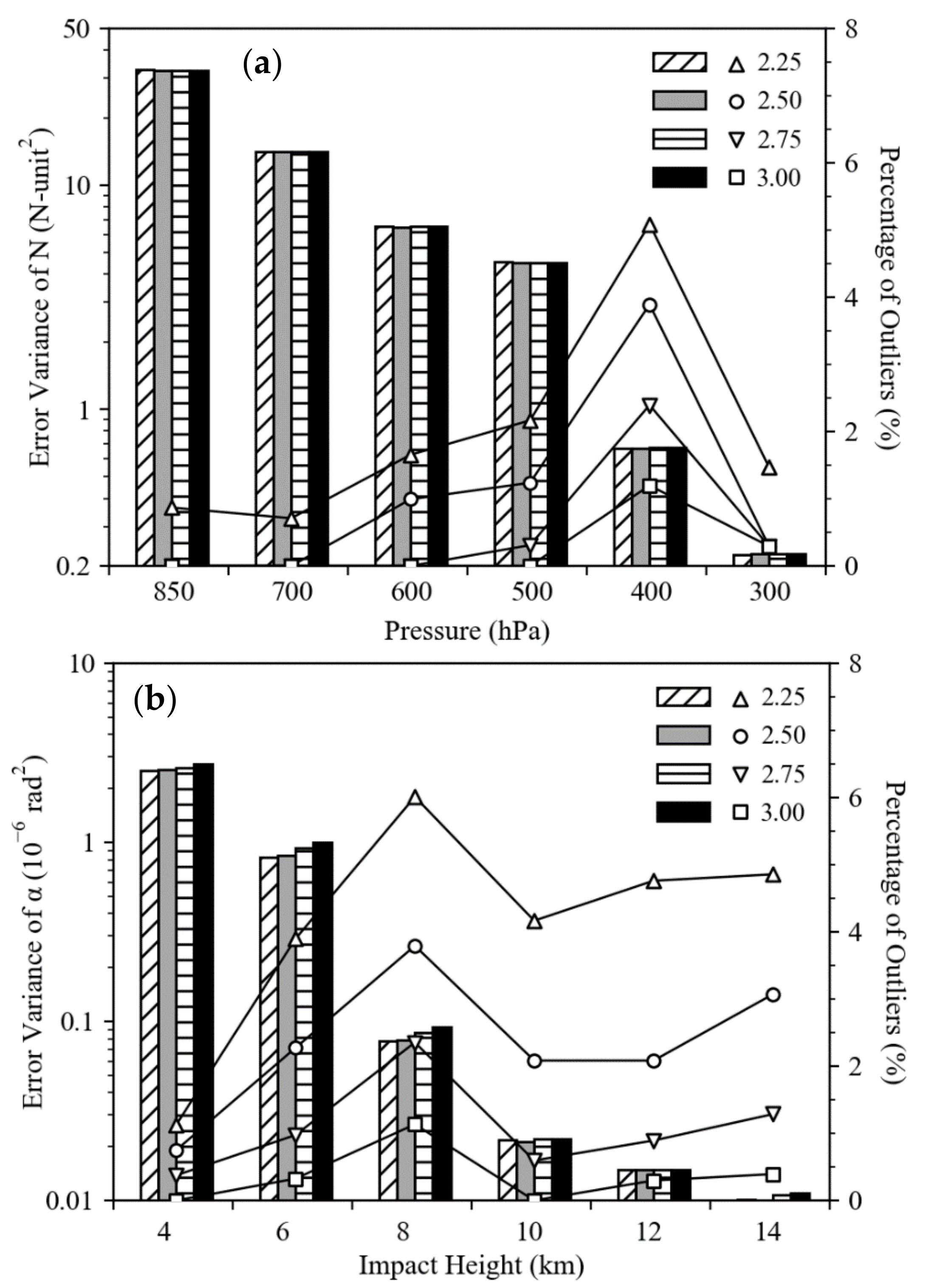
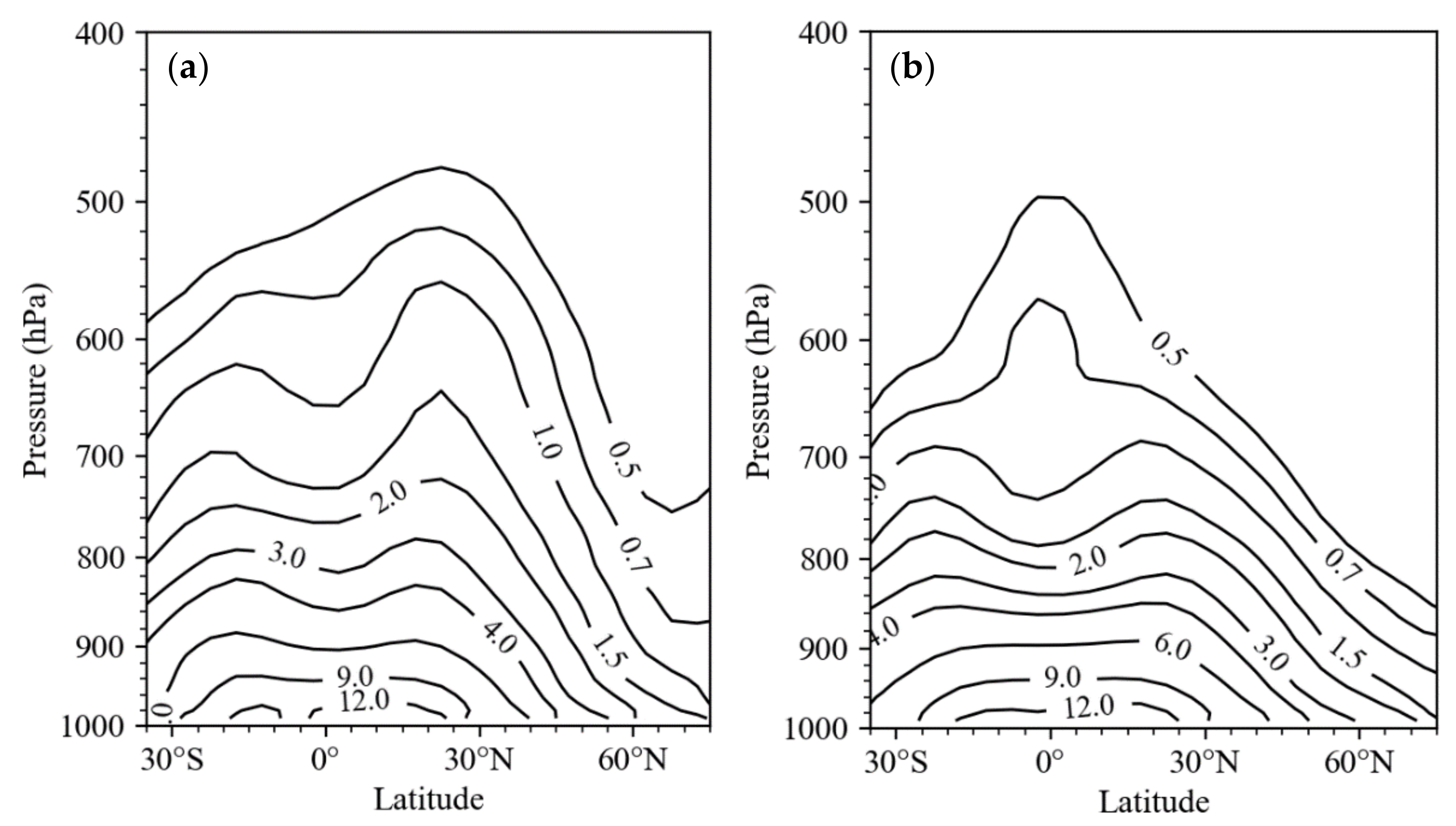
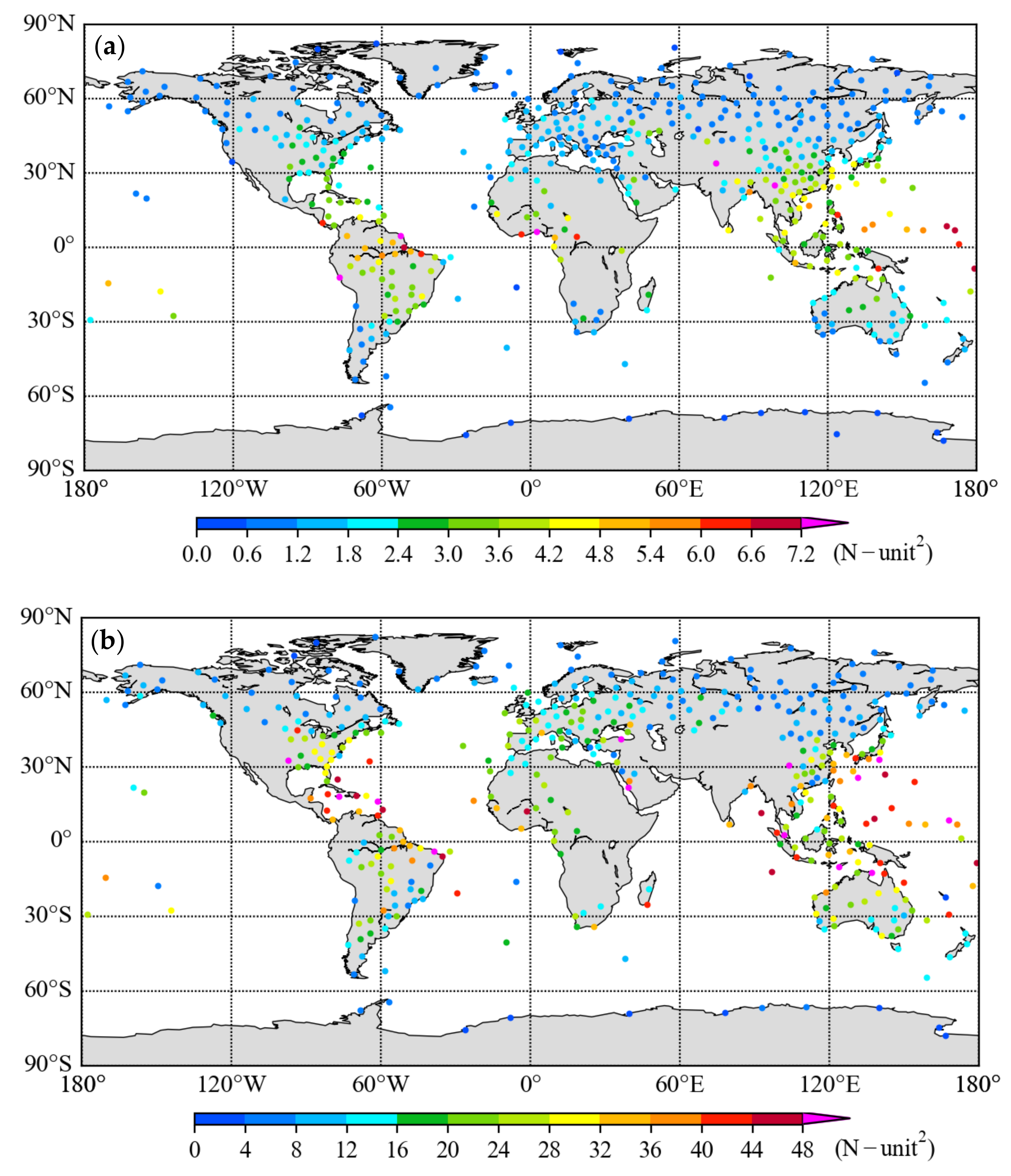
4.1. Error Variances of RO Refractivity
4.2. Error Variances of RO Bending Angle
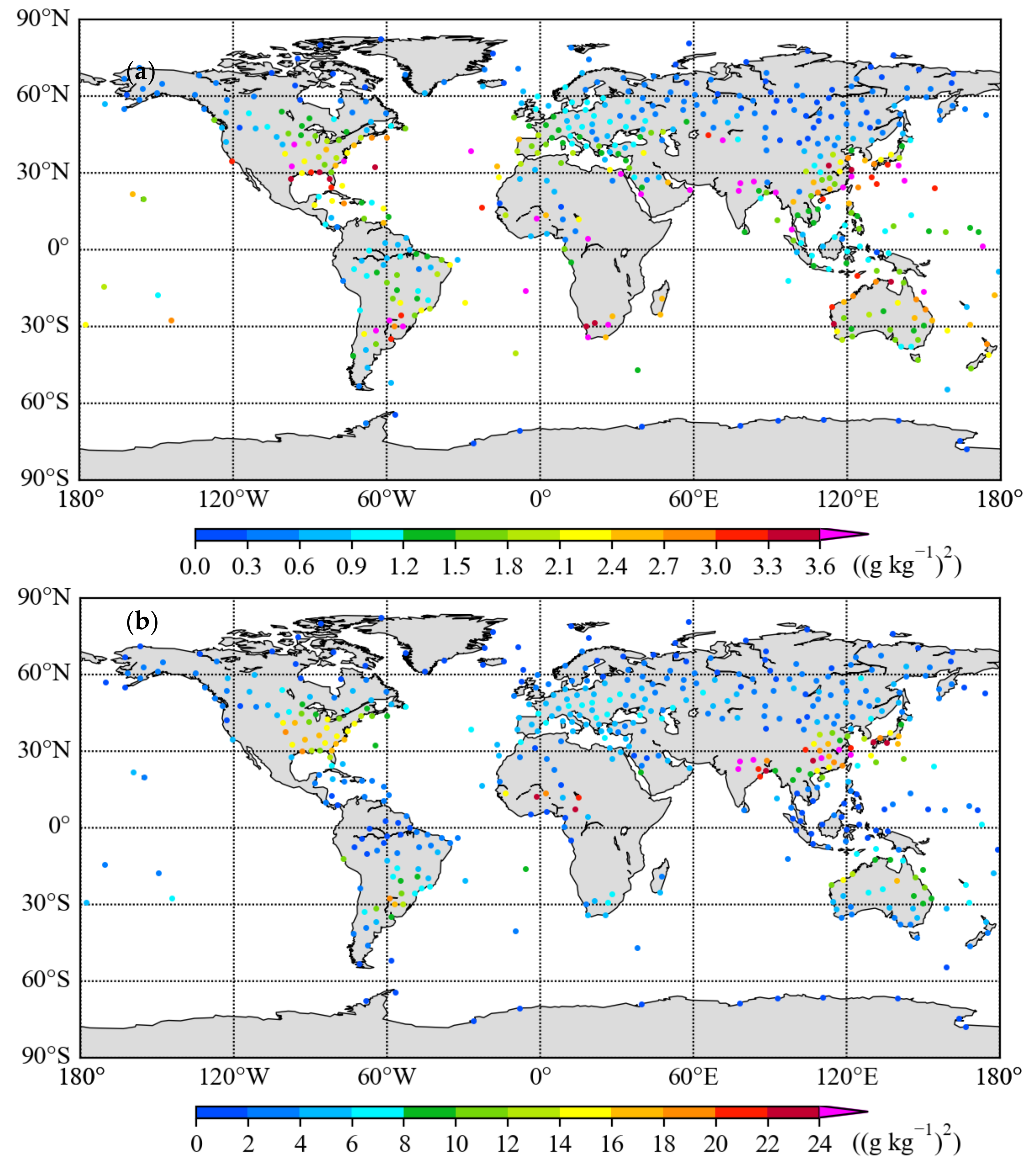
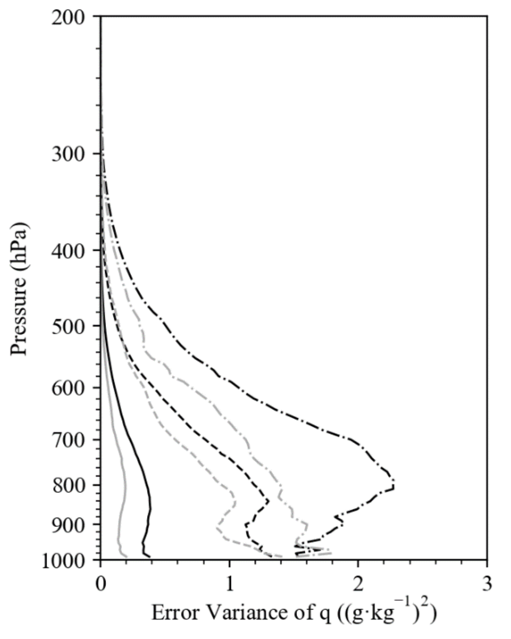
5. Global Error Variances of Radiosonde Observations
6. Discussion
7. Conclusions
Author Contributions
Funding
Conflicts of Interest
Appendix A

| hPa\°N | 0–5 | 5–10 | 10–15 | 15–20 | 20–25 | 25–30 | 30–35 | 35–40 | 40–45 | 45–50 | 50–55 | 55–60 |
|---|---|---|---|---|---|---|---|---|---|---|---|---|
| 990 | 40.46 | 45.67 | 52.15 | 54.00 | 51.65 | 45.70 | 42.35 | 37.44 | 31.39 | 24.23 | 18.91 | 15.50 |
| 980 | 38.52 | 43.31 | 49.44 | 52.09 | 49.76 | 44.66 | 40.10 | 34.66 | 28.26 | 21.92 | 17.28 | 14.37 |
| 970 | 35.11 | 38.86 | 44.69 | 47.96 | 46.57 | 42.40 | 37.86 | 32.30 | 26.08 | 20.40 | 16.37 | 13.70 |
| 960 | 30.52 | 33.04 | 38.60 | 42.39 | 42.17 | 39.29 | 35.42 | 30.19 | 24.41 | 19.33 | 15.76 | 13.26 |
| 950 | 26.82 | 28.52 | 33.15 | 36.61 | 37.36 | 35.87 | 32.91 | 28.28 | 23.05 | 18.44 | 15.16 | 12.80 |
| 940 | 25.87 | 26.69 | 29.30 | 31.77 | 33.27 | 32.99 | 30.70 | 26.58 | 21.89 | 17.67 | 14.58 | 12.34 |
| 930 | 26.64 | 26.63 | 27.35 | 28.90 | 30.81 | 31.19 | 29.11 | 25.27 | 21.00 | 17.06 | 14.09 | 11.90 |
| 920 | 27.85 | 27.57 | 27.21 | 28.04 | 29.88 | 30.36 | 28.20 | 24.39 | 20.31 | 16.55 | 13.65 | 11.49 |
| 910 | 29.04 | 28.98 | 28.23 | 28.46 | 29.76 | 30.00 | 27.69 | 23.77 | 19.77 | 16.10 | 13.25 | 11.11 |
| 900 | 29.95 | 30.31 | 29.59 | 29.25 | 29.77 | 29.60 | 27.15 | 23.22 | 19.29 | 15.71 | 12.92 | 10.78 |
| 890 | 30.54 | 31.40 | 30.90 | 30.06 | 29.71 | 29.03 | 26.52 | 22.69 | 18.86 | 15.36 | 12.61 | 10.49 |
| 880 | 30.74 | 32.17 | 31.98 | 30.75 | 29.60 | 28.44 | 25.90 | 22.17 | 18.43 | 15.04 | 12.33 | 10.22 |
| 870 | 30.62 | 32.65 | 32.81 | 31.34 | 29.55 | 27.93 | 25.28 | 21.61 | 18.01 | 14.73 | 12.05 | 9.96 |
| 860 | 30.36 | 32.89 | 33.40 | 31.74 | 29.37 | 27.31 | 24.59 | 21.01 | 17.52 | 14.36 | 11.75 | 9.69 |
| 850 | 30.14 | 32.90 | 33.56 | 31.66 | 28.77 | 26.49 | 23.79 | 20.26 | 16.88 | 13.90 | 11.39 | 9.38 |
| 840 | 29.88 | 32.55 | 33.20 | 31.03 | 27.83 | 25.50 | 22.85 | 19.39 | 16.20 | 13.44 | 11.03 | 9.05 |
| 830 | 29.48 | 31.85 | 32.39 | 30.00 | 26.71 | 24.43 | 21.87 | 18.60 | 15.67 | 13.06 | 10.70 | 8.75 |
| 820 | 28.78 | 30.80 | 31.21 | 28.78 | 25.61 | 23.46 | 21.05 | 18.00 | 15.22 | 12.69 | 10.39 | 8.46 |
| 810 | 27.72 | 29.50 | 29.85 | 27.54 | 24.61 | 22.59 | 20.32 | 17.38 | 14.67 | 12.23 | 10.02 | 8.15 |
| 800 | 26.55 | 28.21 | 28.49 | 26.29 | 23.49 | 21.54 | 19.38 | 16.56 | 13.96 | 11.68 | 9.60 | 7.82 |
| 790 | 25.49 | 27.04 | 27.17 | 24.98 | 22.19 | 20.29 | 18.24 | 15.60 | 13.19 | 11.08 | 9.15 | 7.47 |
| 780 | 24.43 | 25.86 | 25.94 | 23.81 | 21.04 | 19.16 | 17.18 | 14.71 | 12.45 | 10.49 | 8.70 | 7.13 |
| 770 | 23.21 | 24.63 | 24.83 | 22.86 | 20.19 | 18.31 | 16.32 | 13.96 | 11.81 | 9.97 | 8.29 | 6.81 |
| 760 | 21.97 | 23.42 | 23.74 | 21.94 | 19.46 | 17.60 | 15.61 | 13.32 | 11.27 | 9.52 | 7.93 | 6.51 |
| 750 | 20.94 | 22.28 | 22.56 | 20.87 | 18.61 | 16.82 | 14.88 | 12.71 | 10.76 | 9.11 | 7.60 | 6.23 |
| 740 | 20.09 | 21.20 | 21.29 | 19.64 | 17.58 | 15.91 | 14.12 | 12.09 | 10.25 | 8.70 | 7.26 | 5.95 |
| 730 | 19.12 | 20.03 | 19.96 | 18.33 | 16.46 | 14.96 | 13.36 | 11.47 | 9.72 | 8.26 | 6.90 | 5.67 |
| 720 | 18.02 | 18.82 | 18.62 | 17.08 | 15.40 | 14.06 | 12.63 | 10.86 | 9.19 | 7.80 | 6.53 | 5.38 |
| 710 | 16.96 | 17.66 | 17.39 | 16.00 | 14.47 | 13.22 | 11.90 | 10.24 | 8.66 | 7.35 | 6.16 | 5.10 |
| 700 | 16.02 | 16.60 | 16.30 | 15.08 | 13.65 | 12.43 | 11.16 | 9.61 | 8.14 | 6.93 | 5.82 | 4.83 |
| 690 | 15.16 | 15.59 | 15.24 | 14.15 | 12.83 | 11.66 | 10.43 | 8.99 | 7.65 | 6.53 | 5.50 | 4.57 |
| 680 | 14.35 | 14.61 | 14.22 | 13.19 | 12.01 | 10.94 | 9.76 | 8.42 | 7.19 | 6.15 | 5.19 | 4.30 |
| 670 | 13.59 | 13.75 | 13.29 | 12.28 | 11.27 | 10.34 | 9.19 | 7.90 | 6.74 | 5.77 | 4.86 | 4.02 |
| 660 | 12.92 | 13.01 | 12.49 | 11.52 | 10.68 | 9.82 | 8.67 | 7.41 | 6.30 | 5.37 | 4.53 | 3.75 |
| 650 | 12.25 | 12.27 | 11.69 | 10.78 | 10.07 | 9.26 | 8.13 | 6.91 | 5.85 | 4.98 | 4.19 | 3.49 |
| 640 | 11.52 | 11.44 | 10.83 | 9.99 | 9.38 | 8.63 | 7.54 | 6.40 | 5.42 | 4.61 | 3.88 | 3.23 |
| 630 | 10.83 | 10.69 | 10.04 | 9.25 | 8.70 | 7.99 | 6.95 | 5.90 | 5.03 | 4.27 | 3.59 | 2.98 |
| 620 | 10.25 | 10.09 | 9.39 | 8.64 | 8.14 | 7.43 | 6.42 | 5.45 | 4.66 | 3.95 | 3.32 | 2.76 |
| 610 | 9.73 | 9.55 | 8.85 | 8.18 | 7.70 | 6.96 | 5.96 | 5.04 | 4.30 | 3.65 | 3.06 | 2.55 |
| 600 | 9.23 | 9.04 | 8.38 | 7.78 | 7.29 | 6.52 | 5.53 | 4.65 | 3.95 | 3.35 | 2.82 | 2.35 |
| 590 | 8.72 | 8.54 | 7.94 | 7.37 | 6.84 | 6.06 | 5.11 | 4.27 | 3.61 | 3.06 | 2.58 | 2.15 |
| 580 | 8.20 | 8.05 | 7.51 | 6.93 | 6.37 | 5.60 | 4.70 | 3.91 | 3.30 | 2.79 | 2.35 | 1.96 |
| 570 | 7.68 | 7.56 | 7.05 | 6.47 | 5.90 | 5.16 | 4.32 | 3.59 | 3.02 | 2.54 | 2.13 | 1.78 |
| 560 | 7.09 | 7.00 | 6.51 | 5.97 | 5.43 | 4.74 | 3.97 | 3.29 | 2.76 | 2.31 | 1.93 | 1.62 |
| 550 | 6.45 | 6.35 | 5.89 | 5.40 | 4.92 | 4.31 | 3.63 | 3.00 | 2.51 | 2.10 | 1.75 | 1.47 |
| 540 | 5.81 | 5.69 | 5.23 | 4.78 | 4.38 | 3.87 | 3.28 | 2.72 | 2.26 | 1.89 | 1.58 | 1.33 |
| 530 | 5.21 | 5.06 | 4.60 | 4.16 | 3.83 | 3.42 | 2.93 | 2.43 | 2.02 | 1.69 | 1.42 | 1.20 |
| 520 | 4.65 | 4.49 | 4.02 | 3.60 | 3.32 | 3.00 | 2.58 | 2.15 | 1.79 | 1.51 | 1.28 | 1.09 |
| 510 | 4.13 | 3.96 | 3.51 | 3.13 | 2.91 | 2.64 | 2.28 | 1.91 | 1.60 | 1.36 | 1.16 | 0.99 |
| 500 | 3.65 | 3.48 | 3.07 | 2.76 | 2.57 | 2.34 | 2.03 | 1.70 | 1.43 | 1.22 | 1.04 | 0.90 |
| 490 | 3.19 | 3.02 | 2.67 | 2.42 | 2.27 | 2.07 | 1.79 | 1.50 | 1.27 | 1.09 | 0.94 | 0.82 |
| 480 | 2.76 | 2.59 | 2.31 | 2.11 | 1.99 | 1.82 | 1.58 | 1.32 | 1.12 | 0.97 | 0.84 | 0.75 |
| 470 | 2.36 | 2.21 | 1.98 | 1.83 | 1.74 | 1.60 | 1.39 | 1.16 | 0.98 | 0.86 | 0.76 | 0.68 |
| 460 | 2.02 | 1.89 | 1.70 | 1.59 | 1.52 | 1.40 | 1.22 | 1.02 | 0.87 | 0.77 | 0.68 | 0.62 |
| 450 | 1.73 | 1.63 | 1.46 | 1.38 | 1.33 | 1.23 | 1.07 | 0.90 | 0.77 | 0.68 | 0.61 | 0.56 |
| 440 | 1.47 | 1.39 | 1.26 | 1.19 | 1.15 | 1.07 | 0.93 | 0.79 | 0.68 | 0.61 | 0.55 | 0.51 |
| 430 | 1.24 | 1.17 | 1.06 | 1.01 | 0.99 | 0.92 | 0.81 | 0.69 | 0.60 | 0.54 | 0.50 | 0.46 |
| 420 | 1.04 | 0.98 | 0.89 | 0.85 | 0.84 | 0.79 | 0.70 | 0.60 | 0.53 | 0.49 | 0.45 | 0.43 |
| 410 | 0.88 | 0.83 | 0.75 | 0.72 | 0.72 | 0.69 | 0.61 | 0.53 | 0.48 | 0.45 | 0.42 | 0.40 |
| 400 | 0.74 | 0.70 | 0.64 | 0.62 | 0.63 | 0.60 | 0.54 | 0.47 | 0.44 | 0.41 | 0.39 | 0.37 |
| IH\°N | 0–5 | 5–10 | 10–15 | 15–20 | 20–25 | 25–30 | 30–35 | 35–40 | 40–45 | 45–50 | 50–55 | 55–60 |
|---|---|---|---|---|---|---|---|---|---|---|---|---|
| 2.1 | −999 | −999 | −999 | −999 | −999 | −999 | −999 | −999 | −999 | −999 | 1.07 | 1.63 |
| 2.3 | −999 | −999 | −999 | −999 | −999 | −999 | 4.50 | 4.41 | 4.61 | 2.72 | 2.25 | 2.02 |
| 2.5 | −999 | 4.89 | −999 | −999 | 11.20 | 6.83 | 6.70 | 5.72 | 4.53 | 3.45 | 2.72 | 2.23 |
| 2.7 | 7.68 | 7.10 | 7.67 | 9.83 | 9.41 | 8.22 | 7.02 | 5.67 | 4.36 | 3.35 | 2.63 | 2.12 |
| 2.9 | 6.74 | 6.71 | 7.21 | 7.71 | 7.59 | 6.98 | 6.07 | 4.92 | 3.82 | 2.97 | 2.37 | 1.93 |
| 3.1 | 5.89 | 6.06 | 6.50 | 6.79 | 6.65 | 6.14 | 5.33 | 4.33 | 3.39 | 2.66 | 2.14 | 1.75 |
| 3.3 | 5.75 | 6.02 | 6.35 | 6.45 | 6.17 | 5.58 | 4.78 | 3.89 | 3.08 | 2.45 | 1.98 | 1.60 |
| 3.5 | 5.90 | 6.15 | 6.33 | 6.19 | 5.71 | 5.03 | 4.28 | 3.51 | 2.82 | 2.25 | 1.81 | 1.45 |
| 3.7 | 5.75 | 5.94 | 5.97 | 5.66 | 5.10 | 4.45 | 3.78 | 3.12 | 2.50 | 2.00 | 1.59 | 1.26 |
| 3.9 | 5.31 | 5.39 | 5.31 | 4.96 | 4.44 | 3.86 | 3.28 | 2.69 | 2.16 | 1.73 | 1.37 | 1.09 |
| 4.1 | 4.71 | 4.78 | 4.68 | 4.35 | 3.85 | 3.33 | 2.80 | 2.28 | 1.82 | 1.44 | 1.15 | 0.91 |
| 4.3 | 4.21 | 4.28 | 4.19 | 3.90 | 3.46 | 2.97 | 2.46 | 1.97 | 1.54 | 1.21 | 0.96 | 0.77 |
| 4.5 | 3.70 | 3.77 | 3.73 | 3.50 | 3.12 | 2.66 | 2.18 | 1.72 | 1.35 | 1.05 | 0.83 | 0.66 |
| 4.7 | 3.21 | 3.29 | 3.26 | 3.06 | 2.73 | 2.33 | 1.90 | 1.51 | 1.19 | 0.93 | 0.73 | 0.57 |
| 4.9 | 2.78 | 2.82 | 2.79 | 2.63 | 2.37 | 2.02 | 1.65 | 1.30 | 1.02 | 0.80 | 0.62 | 0.49 |
| 5.1 | 2.42 | 2.44 | 2.41 | 2.29 | 2.07 | 1.78 | 1.44 | 1.13 | 0.87 | 0.68 | 0.53 | 0.41 |
| 5.3 | 2.12 | 2.15 | 2.12 | 2.02 | 1.83 | 1.57 | 1.26 | 0.98 | 0.75 | 0.57 | 0.44 | 0.34 |
| 5.5 | 1.86 | 1.88 | 1.84 | 1.74 | 1.58 | 1.35 | 1.09 | 0.84 | 0.64 | 0.49 | 0.38 | 0.29 |
| 5.7 | 1.67 | 1.66 | 1.61 | 1.51 | 1.36 | 1.16 | 0.93 | 0.72 | 0.54 | 0.42 | 0.32 | 0.25 |
| 5.9 | 1.50 | 1.49 | 1.43 | 1.33 | 1.19 | 1.00 | 0.79 | 0.61 | 0.46 | 0.35 | 0.28 | 0.21 |
| 6.1 | 1.34 | 1.33 | 1.28 | 1.18 | 1.04 | 0.86 | 0.68 | 0.51 | 0.39 | 0.30 | 0.23 | 0.18 |
| 6.3 | 1.21 | 1.20 | 1.14 | 1.04 | 0.91 | 0.75 | 0.58 | 0.44 | 0.33 | 0.25 | 0.19 | 0.14 |
| 6.5 | 1.06 | 1.03 | 0.97 | 0.88 | 0.77 | 0.64 | 0.49 | 0.37 | 0.27 | 0.20 | 0.15 | 0.12 |
| 6.7 | 0.87 | 0.84 | 0.78 | 0.71 | 0.63 | 0.52 | 0.40 | 0.30 | 0.22 | 0.16 | 0.12 | 0.10 |
| 6.9 | 0.67 | 0.65 | 0.59 | 0.54 | 0.48 | 0.40 | 0.31 | 0.24 | 0.17 | 0.13 | 0.10 | 0.08 |
| 7.1 | 0.52 | 0.50 | 0.45 | 0.40 | 0.36 | 0.30 | 0.24 | 0.18 | 0.13 | 0.10 | 0.08 | 0.06 |
| 7.3 | 0.41 | 0.39 | 0.35 | 0.31 | 0.28 | 0.23 | 0.19 | 0.14 | 0.10 | 0.08 | 0.06 | 0.05 |
| 7.5 | 0.33 | 0.31 | 0.28 | 0.25 | 0.23 | 0.19 | 0.15 | 0.11 | 0.08 | 0.06 | 0.05 | 0.04 |
| 7.7 | 0.28 | 0.26 | 0.23 | 0.21 | 0.19 | 0.16 | 0.13 | 0.09 | 0.07 | 0.05 | 0.04 | 0.03 |
| 7.9 | 0.23 | 0.21 | 0.19 | 0.18 | 0.16 | 0.13 | 0.11 | 0.08 | 0.06 | 0.04 | 0.03 | 0.03 |
| 8.1 | 0.19 | 0.18 | 0.16 | 0.15 | 0.13 | 0.11 | 0.09 | 0.07 | 0.05 | 0.04 | 0.03 | 0.02 |
| 8.3 | 0.16 | 0.15 | 0.14 | 0.13 | 0.11 | 0.10 | 0.08 | 0.06 | 0.04 | 0.03 | 0.02 | 0.02 |
| 8.5 | 0.12 | 0.12 | 0.11 | 0.10 | 0.09 | 0.08 | 0.06 | 0.05 | 0.04 | 0.03 | 0.02 | 0.02 |
| 8.7 | 0.09 | 0.09 | 0.09 | 0.08 | 0.07 | 0.06 | 0.05 | 0.04 | 0.03 | 0.02 | 0.02 | 0.02 |
| 8.9 | 0.08 | 0.08 | 0.07 | 0.07 | 0.06 | 0.05 | 0.04 | 0.03 | 0.03 | 0.02 | 0.02 | 0.02 |
| 9.1 | 0.07 | 0.06 | 0.06 | 0.06 | 0.05 | 0.04 | 0.04 | 0.03 | 0.02 | 0.02 | 0.02 | 0.01 |
| 9.3 | 0.05 | 0.05 | 0.05 | 0.05 | 0.04 | 0.04 | 0.03 | 0.02 | 0.02 | 0.02 | 0.01 | 0.01 |
| 9.5 | 0.04 | 0.04 | 0.04 | 0.04 | 0.03 | 0.03 | 0.03 | 0.02 | 0.02 | 0.01 | 0.01 | 0.01 |
| 9.7 | 0.03 | 0.03 | 0.03 | 0.03 | 0.03 | 0.02 | 0.02 | 0.02 | 0.01 | 0.01 | 0.01 | 0.01 |
| 9.9 | 0.02 | 0.02 | 0.02 | 0.02 | 0.02 | 0.02 | 0.02 | 0.01 | 0.01 | 0.01 | 0.01 | 0.01 |
| 10.1 | 0.01 | 0.01 | 0.01 | 0.01 | 0.01 | 0.01 | 0.01 | 0.01 | 0.01 | 0.01 | 0.01 | 0.01 |
| 10.3 | 0.01 | 0.01 | 0.01 | 0.01 | 0.01 | 0.01 | 0.01 | 0.01 | 0.01 | 0.01 | 0.01 | 0.01 |
| 10.5 | 0.01 | 0.01 | 0.01 | 0.01 | 0.01 | 0.01 | 0.01 | 0.01 | 0.01 | 0.01 | 0.01 | 0.01 |
| 10.7 | 0.01 | 0.01 | 0.01 | 0.01 | 0.01 | 0.01 | 0.01 | 0.01 | 0.01 | 0.01 | 0.01 | 0.01 |
| 10.9 | 0.01 | 0.01 | 0.01 | 0.01 | 0.01 | 0.01 | 0.01 | 0.01 | 0.01 | 0.01 | 0.01 | 0.01 |
References
- Kuo, Y.-H.; Schreiner, W.S.; Rossiter, D.L.; Wang, J.; Zhang, Y. Comparison of GPS radio occultation soundings with radiosondes. Geophys. Res. Lett. 2005, 32. [Google Scholar] [CrossRef] [Green Version]
- Ho, S.-P.; Zhou, X.; Kuo, Y.; Hunt, D.; Wang, J. Global Evaluation of Radiosonde Water Vapor Systematic Biases using GPS Radio Occultation from COSMIC and ECMWF Analysis. Remote. Sens. 2010, 2, 1320–1330. [Google Scholar] [CrossRef] [Green Version]
- Vergados, P.; Mannucci, A.J.; Ao, C.O. Assessing the performance of GPS radio occultation measurements in retrieving tropospheric humidity in cloudiness: A comparison study with radiosondes, ERA-Interim, and AIRS data sets. J. Geophys. Res. Atmos. 2014, 119, 7718–7731. [Google Scholar] [CrossRef]
- Kursinski, E.R.; Hajj, G.A.; Schofield, J.T.; Linfield, R.P.; Hardy, K.R. Observing Earth’s atmosphere with radio occultation measurements using the Global Positioning System. J. Geophys. Res. Space Phys. 1997, 102, 23429–23465. [Google Scholar] [CrossRef]
- Anthes, R.A.; Bernhardt, P.A.; Chen, Y.; Cucurull, L.; Dymond, K.F.; Ector, D.; Healy, S.B.; Ho, S.-P.; Hunt, D.C.; Kuo, Y.; et al. The COSMIC/FORMOSAT-3 Mission: Early Results. Bull. Am. Meteorol. Soc. 2008, 89, 313–334. [Google Scholar] [CrossRef]
- Ho, S.-P.; Anthes, R.A.; Ao, C.O.; Healy, S.; Horanyi, A.; Hunt, D.; Mannucci, A.J.; Pedatella, N.; Randel, W.J.; Simmons, A.; et al. The COSMIC/FORMOSAT-3 Radio Occultation Mission after 12 Years: Accomplishments, Remaining Challenges, and Potential Impacts of COSMIC-2. Bull. Am. Meteorol. Soc. 2020, 101, E1107–E1136. [Google Scholar] [CrossRef] [Green Version]
- Schreiner, W.S.; Weiss, J.; Anthes, R.; Braun, J.; Chu, V.; Fong, J.; Hunt, D.; Kuo, Y.; Meehan, T.; Serafino, W.; et al. COSMIC-2 Radio Occultation Constellation: First Results. Geophys. Res. Lett. 2020, 47, 086841. [Google Scholar] [CrossRef]
- Benjamin, S.G.; Jamison, B.D.; Moninger, W.R.; Sahm, S.R.; Schwartz, B.E.; Schlatter, T.W. Relative Short-Range Forecast Impact from Aircraft, Profiler, Radiosonde, VAD, GPS-PW, METAR, and Mesonet Observations via the RUC Hourly Assimilation Cycle. Mon. Weather. Rev. 2010, 138, 1319–1343. [Google Scholar] [CrossRef]
- Healy, S. Forecast impact experiment with a constellation of GPS radio occultation receivers. Atmos. Sci. Lett. 2008, 9, 111–118. [Google Scholar] [CrossRef]
- Rennie, M.P. The impact of GPS radio occultation assimilation at the Met Office. Q. J. R. Meteorol. Soc. 2010, 136, 116–131. [Google Scholar] [CrossRef]
- Liu, H.; Kuo, Y.; Sokolovskiy, S.V.; Zou, X.; Zeng, Z.; Hsiao, L.-F.; Ruston, B.C. A Quality Control Procedure Based on Bending Angle Measurement Uncertainty for Radio Occultation Data Assimilation in the Tropical Lower Troposphere. J. Atmos. Ocean. Technol. 2018, 35, 2117–2131. [Google Scholar] [CrossRef]
- Sato, K.; Inoue, J.; Yamazaki, A.; Hirasawa, N.; Sugiura, K.; Yamada, K. Antarctic Radiosonde Observations Reduce Uncertainties and Errors in Reanalyses and Forecasts over the Southern Ocean: An Extreme Cyclone Case. Adv. Atmos. Sci. 2020, 37, 431–440. [Google Scholar] [CrossRef] [Green Version]
- Zou, X. Three-Dimensional Variational Data Assimilation; Elsevier BV: Amsterdam, NY, USA, 2020; pp. 135–161. [Google Scholar]
- Shao, H.; Hajj, G.A.; Zou, X. Test of a non-local excess phase delay operator for GPS radio occultation data assimilation. J. Appl. Remote Sens. 2009, 3, 033508. [Google Scholar] [CrossRef]
- Geer, A.J.; Bauer, P. Observation errors in all-sky data assimilation. Q. J. R. Meteorol. Soc. 2011, 137, 2024–2037. [Google Scholar] [CrossRef]
- Shao, H.; Zou, X. The impact of observational weighting on the assimilation of GPS/MET bending angle. J. Geophys. Res. Space Phys. 2002, 107, ACL 19-1–ACL 19-28. [Google Scholar] [CrossRef]
- Kuo, Y.-H.; Wee, T.-K.; Sokolovskiy, S.; Rocken, C.; Schreiner, W.; Hunt, D.; Anthes, R. Inversion and Error Estimation of GPS Radio Occultation Data. J. Meteorol. Soc. Jpn. 2004, 82, 507–531. [Google Scholar] [CrossRef] [Green Version]
- Chen, S.-Y.; Huang, C.-Y.; Kuo, Y.-H.; Sokolovskiy, S. Observational Error Estimation of FORMOSAT-3/COSMIC GPS Radio Occultation Data. Mon. Weather Rev. 2011, 139, 853–865. [Google Scholar] [CrossRef] [Green Version]
- Steiner, A.K. Error analysis for GNSS radio occultation data based on ensembles of profiles from end-to-end simulations. J. Geophys. Res. Space Phys. 2005, 110. [Google Scholar] [CrossRef]
- Poli, P.; Moll, P.; Puech, D.; Rabier, F.; Healy, S.B. Quality Control, Error Analysis, and Impact Assessment of FORMOSAT-3/COSMIC in Numerical Weather Prediction. Terr. Atmos. Ocean. Sci. 2009, 20, 101. [Google Scholar] [CrossRef] [Green Version]
- Anthes, R.; Rieckh, T. Estimating observation and model error variances using multiple data sets. Atmos. Meas. Tech. 2018, 11, 4239–4260. [Google Scholar] [CrossRef] [Green Version]
- Gray, J.E.; Allan, D.W. A Method for Estimating the Frequency Stability of an Individual Oscillator. In Proceedings of the 28th Annual Symposium on Frequency Control, Institute of Electrical and Electronics Engineers (IEEE), Atlantic City, NJ, USA, 29–31 May 1974; pp. 243–246. [Google Scholar]
- Xu, X.; Zou, X. Estimating GPS radio occultation observation error standard deviations over China using the three-cornered hat method. Q. J. R. Meteorol. Soc. 2020. [Google Scholar] [CrossRef]
- Kishore, P.; Medineni, V.R.; Namboothiri, S.; Velicogna, I.; Basha, G.; Jiang, J.; Igarashi, K.; Rao, N.V.; Sivakumar, V. Global (50°S–50°N) distribution of water vapor observed by COSMIC GPS RO: Comparison with GPS radiosonde, NCEP, ERA-Interim, and JRA-25 reanalysis data sets. J. Atmos. Sol.-Terrestrial Phys. 2011, 73, 1849–1860. [Google Scholar] [CrossRef] [Green Version]
- Ladstädter, F.; Steiner, A.K.; Schwarz, M.; Kirchengast, G. Climate intercomparison of GPS radio occultation, RS90/92 radiosondes and GRUAN from 2002 to 2013. Atmos. Meas. Tech. 2015, 8, 1819–1834. [Google Scholar] [CrossRef] [Green Version]
- Ho, S.-P.; Peng, L.; Vömel, H. Characterization of the long-term radiosonde temperature biases in the upper troposphere and lower stratosphere using COSMIC and Metop-A/GRAS data from 2006 to 2014. Atmos. Chem. Phys. Discuss. 2017, 17, 4493–4511. [Google Scholar] [CrossRef] [Green Version]
- Durre, I.; Vose, R.S.; Wuertz, D.B. Overview of the Integrated Global Radiosonde Archive. J. Clim. 2006, 19, 53–68. [Google Scholar] [CrossRef] [Green Version]
- Durre, I.; Vose, R.S.; Wuertz, D.B. Robust Automated Quality Assurance of Radiosonde Temperatures. J. Appl. Meteorol. Clim. 2008, 47, 2081–2095. [Google Scholar] [CrossRef]
- Dee, D.P.; Uppala, S.M.; Simmons, A.J.; Berrisford, P.; Poli, P.; Kobayashi, S.; Andrae, U.; Balmaseda, M.A.; Balsamo, G.; Bauer, P.; et al. The ERA-Interim reanalysis: Configuration and performance of the data assimilation system. Q. J. R. Meteorol. Soc. 2011, 137, 553–597. [Google Scholar] [CrossRef]
- Gilpin, S.; Rieckh, T.; Anthes, R. Reducing representativeness and sampling errors in radio occultation–radiosonde comparisons. Atmos. Meas. Tech. 2018, 11, 2567–2582. [Google Scholar] [CrossRef] [Green Version]
- Lohmann, M.S. Analysis of Global Positioning System (GPS) radio occultation measurement errors based on Satellite de Aplicaciones Cientificas-C (SAC-C) GPS radio occultation data recorded in open-loop and phase-locked-loop mode. J. Geophys. Res. Space Phys. 2007, 112. [Google Scholar] [CrossRef] [Green Version]
- Zou, X.; Zeng, Z. A quality control procedure for GPS radio occultation data. J. Geophys. Res. Space Phys. 2006, 111. [Google Scholar] [CrossRef] [Green Version]
- ROM SAF, 2019: The Radio Occultation Processing Package (ROPP) Forward Model Module User Guide, SAF/ROM/METO/UG/ROPP/006. Available online: https://www.romsaf.org/romsaf_ropp_ug_fm.pdf (accessed on 30 June 2019).
- Ingleby, B. An Assessment of Different Radiosonde Types 2015/2016; ECMWF Technical Memoranda 807; ECMWF: Reading, UK, 2017. [Google Scholar] [CrossRef]
- Mitchell, H.L.; Houtekamer, P.L.; Pellerin, G. Ensemble Size, Balance, and Model-Error Representation in an Ensemble Kalman Filter. Mon. Weather. Rev. 2002, 130, 2791–2808. [Google Scholar] [CrossRef] [Green Version]


Publisher’s Note: MDPI stays neutral with regard to jurisdictional claims in published maps and institutional affiliations. |
© 2020 by the authors. Licensee MDPI, Basel, Switzerland. This article is an open access article distributed under the terms and conditions of the Creative Commons Attribution (CC BY) license (http://creativecommons.org/licenses/by/4.0/).
Share and Cite
Xu, X.; Zou, X. Global 3D Features of Error Variances of GPS Radio Occultation and Radiosonde Observations. Remote Sens. 2021, 13, 1. https://doi.org/10.3390/rs13010001
Xu X, Zou X. Global 3D Features of Error Variances of GPS Radio Occultation and Radiosonde Observations. Remote Sensing. 2021; 13(1):1. https://doi.org/10.3390/rs13010001
Chicago/Turabian StyleXu, Xu, and Xiaolei Zou. 2021. "Global 3D Features of Error Variances of GPS Radio Occultation and Radiosonde Observations" Remote Sensing 13, no. 1: 1. https://doi.org/10.3390/rs13010001
APA StyleXu, X., & Zou, X. (2021). Global 3D Features of Error Variances of GPS Radio Occultation and Radiosonde Observations. Remote Sensing, 13(1), 1. https://doi.org/10.3390/rs13010001