1. Introduction
The wide-spread use of 3D models in fields such as architecture, urban planning, and archaeology [
1,
2,
3] means that some professionals cannot generate 3D models without advanced technical knowledge in surveying. In this context, many investigations carried out in recent years have been aimed at the development of new products and working methods that simplify the necessary requirements both for data acquisition and processing, without harming the accuracies of the resulting products [
4,
5,
6]. In parallel, multiple 3D data acquisition systems based on active or passive sensors have appeared in recent decades, obtaining 3D models either as point clouds or textured surfaces. These new systems have revolutionized the possibilities of users, obtaining results that assist in understanding digitized elements and facilitating studies that could hardly be carried out in any other way [
7,
8,
9].
Among the various systems that are commonly used for data acquisition in architecture, urban planning, and archaeology, mid-range terrestrial laser scanners (TLS) [
10] are commonly used, which are survey instruments that use laser pulses to measure distances and a rotating mirror to measure angles, generating a point cloud of the environment with a range of 0.5–300 m and root mean square error (RMS) between 1 and 4 mm. Mobile mapping systems (MMS) [
9,
11] are based on multiple synchronized components, such as LIDAR, IMU, GNSS, cameras, odometers, and so on, with which 3D models can be constructed with up to 2 cm RMS errors. Handheld scanners, normally based on active sensors such as lidar or structured light sensors, are considered MMS. With handheld scanners, data are captured while the user moves through a work area. Lidar-based handheld scanners, which are applicable to the fields of interest in this article, achieve RMSE errors of 1–3 cm, with ranges usually no greater than 150 m [
1]. Finally, we consider photogrammetric techniques [
12] as a perfectly viable and growing means for generating 3D models in the fields of architecture, urban planning, and heritage. Such 3D models have been generated using 10–12 Mpx commercial cameras and commercial photogrammetric software, with a variable distance between 1 and 15 m in these applications, following certain proven capture procedures and conditions [
13,
14], the RMSE of these models ranges from 2 mm for the closest distances to 1 cm for longer distances. In the aerial photogrammetric case [
15,
16], if we consider a flight height of 30 m, the accuracy can reach 2–9 cm.
In the cases of TLS and MMS, in competition between companies to satisfy the market requirements, research has normally been directed towards simplifying the procedures and facilitating the interaction of the instrument with users, creating ever simpler and more user-friendly interfaces. Thus, these technologies can now be used by non-expert users [
9,
17,
18]. Among commercial TLS, we mention the Faro Focus 150, manufactured by FARO Technologies Inc. (Lake Mary, FL, USA); the Leica RTC360, manufactured by Leica geosystems (Heerbrugg, Switzerland); the RIEGL VZ-400i, manufactured by RIEGL Laser Measurement Systems (Horn, Austria); and the Z+F imager, manufactured by Zoller & Frölich GmbH (Wangen im Allgäu, Germany) [
19,
20,
21,
22]. Manufacturers have opted to facilitate their use by simplifying user interfaces, connectivity, and scan pre-registration procedures (automatic or semi-automatic). Still, the reading and loading data processes in the software and the inconvenience of having to process millions of points at once, especially at very high resolutions, is a major challenge for users; especially for non-experts. The most widely used MMS for large-scale scanning and mapping projects in urban, architectural, and archaeological environments are vehicle-based mobile mapping platforms or those that must be transported by backpack or trolley. In the former, we mention the UltraCam Mustang, manufactured by Vexcel Imaging GmbH (Gra, Austria); the Leica Pegasus:Two Ultimate, manufactured by Leica geosystems (Heerbrug, Switzerland); and the Trimble MX9, manufactured by Trimble (Sunnyvale, CA, USA) [
23,
24,
25], which use inertial systems and GNSS for positioning, and are equipped with LIDAR profilers with high scanning speeds (up to 500 scans/s) and 360 cameras to achieve street-level scenery with geo-positioned panoramic imagery. The latter type (i.e., systems transported by a backpack or by a trolley) are usually used for indoor/outdoor middle-scale scanning and mapping projects with difficult access (buildings, urban centers, construction areas, caves, and so on). These products include systems based on different technologies, including active capture sensors (e.g., Lidar) and passive sensors (e.g., cameras), as well as GNSS and IMU systems, which assist the system in positioning and orienting itself. In this type of product, we mention the Leica Pegasus: Backpack, manufactured by Leica Geosystems (Heerbrugg, Switzerland); the bMS3D LD5+, manufactured by Viametris (Louverné, France); and the trimble Indoor Mobile Mapping solution (TIMMS), manufactured by Applanix (Richmond Hill, ON, Canada) [
26,
27,
28].
Data acquisition in MMS is automatic and normally easy and fast. However, there is still the inconvenience of having to manage clouds of millions of points, increasing the time required in data processing [
29]; in addition to the fact that the price of the equipment is usually high, ranging between €350,000 and €650,000 for vehicle-based mobile mapping platform systems and €60,000 and €350,000 for systems carried by a backpack or trolley.
However, in the case of systems based on photogrammetric techniques, many investigations have been aimed at both simplifying data processing and obtaining the final results as automatically as possible. In the dynamics of simplification such that photogrammetry can be used by non-experts, the use of modern smart phones and tablets to capture high-resolution images [
30,
31,
32], following which the obtained data are processed in the cloud. This process has been used in applications such as the Photogrammetry App created by Linearis HmbH & Co (Braunschweig, Germany) and ContextCapture mobile created by Bentley systems Incorporated (Exton, PA, USA) [
33,
34], among others. In general terms, the technical knowledge required of the user has been practically reduced to adapting the parameters of the camera to manage the scene lighting conditions and ensuring good camera poses geometry [
35]; therefore, a semi-automated process is followed using the captured information, in which the user practically does not intervene [
32]. In this line, companies have focused their objectives on achieving data capture without prior technical knowledge and almost fully automatic data processing. In short, their main goal is achieving fast and accurate data capture with which high-quality end products can be obtained, while being accessible to a non-specialized user. Thus, some manufacturers have chosen to use photogrammetric techniques in their MMS capture systems (instead of using laser scanning systems), such as the Trimble MX7 manufactured by Trimble (Sunnyvale, CA, USA) [
36], which consists of a vehicle-mounted photogrammetric system equipped with a set of six 5 megapixel cameras using GNSS and inertial referencing system for precise positioning; as well as the imajing 3D Pro system from imaging SAS (Labège, France) [
37], in which photogrammetric tools are used to process the 2D images obtained by a sensor which, for precise and continuous positioning, is equipped with an inertial system, a GNSS receiver, and a barometric sensor, thus constituting a complete portable mobile mapping system for high-speed data collection.
From the above, it follows that the most commonly used positioning and measurement systems are based on inertial systems, GNSS, cameras, and LIDAR. However, some recent research [
1,
38,
39] has been directed at combining laser measurement systems with positioning systems based on visual odometry (VO) or simultaneous localization and mapping (SLAM) techniques. With this type of design, the company Geoslam (Nottingham, UK) has launched ZEB systems with three configurations—Revo, Horizon, and Discovery—which are handheld or carried in a backpack, and have capture ranges between 5–100 m and relative accuracies ranging between 1–3 cm. Videogrammetric 3D reconstruction through smartphones using a 3D-based images selection have been also explored [
40]. In this paper, VisualSLAM [
41] and photogrammetry techniques using high-resolution images from an industrial video-camera have been combined for 3D reconstruction; 3D-based and ad hoc algorithms has been used for an optimal images selection and for the calculations, to obtain longer data sets and more complex 3D and precise 3D scenarios. To explore this possibility, a new system has been designed: A simple handheld imaging scanner based on two commercial cameras, one of which is used to compute the camera position in real time using the VisualSLAM algorithm; the other camera is a high-resolution frame recorder, which continuously saves images of the scene which, using photogrammetry, is used to generate a 3D color point cloud. To evaluate the effectiveness of the proposed system, a set of three studies were performed in the House of Mitreo (Mérida, Spain), a dwelling from Roman times with ongoing archaeological excavations. In these experiments, different aspects such as the data acquisition and processing time, the average density of the point clouds, and the level of accuracy (LOA) of each point cloud, are evaluated, taking as reference a set of 150 targets distributed throughout the entire area, whose coordinates were observed with a total station. Likewise, the same areas were scanned with a Focus3D X 330 laser scanner manufactured by FARO Technologies Inc. (Lake Mary, FL, USA) [
19], in order to compare the results obtained with the proposed system and ensure the absence of systematic errors between both systems. The results obtained with acquisition times and human intervention in the data processing using the proposed system were 31 and 0 min, respectively (compared to 520 and 97 min with the laser scanner), the mean point cloud density value is 1.6 points/mm (compared to 0.3 pts/mm with the laser scanner), and accuracy values between 5–6 mm (RMSEs) to evaluate LOA (compared to the 6–7 mm obtained with the laser scanner). In addition, circular statistics were computed to confirm of the absence of systematic errors between both systems, stressing the feasibility of the proposed system in archaeological environments.
This paper is divided into four sections: In
Section 2, the proposed system is described, from the first idea to its current state. In
Section 3, the experimental tests carried out with the system are described, and the results are also presented. Finally,
Section 4 presents our final conclusions.
2. Materials and Methods
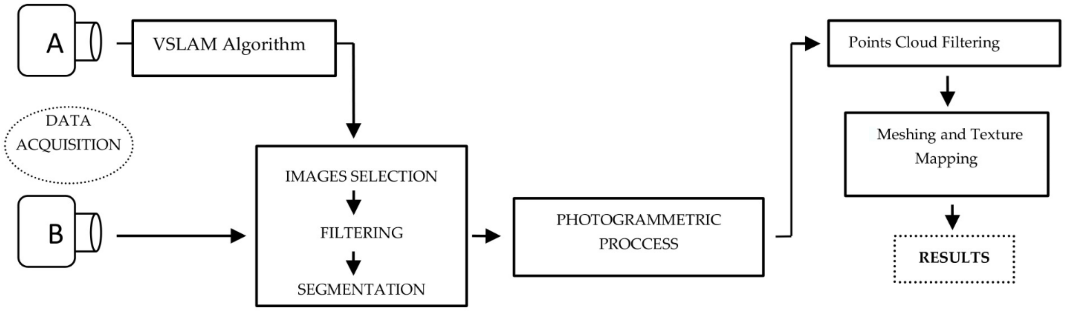
The process of point cloud generation by the proposed system, which combines VisualSLAM and photogrammetry, is shown in
Figure 1. This scheme is based on simultaneous video capture by two cameras, A and B: With the images obtained with camera A, the camera pose is computed in real time (applying the VSLAM algorithm) and, therefore, the camera trajectory data are obtained. High-resolution images are extracted from the video obtained by camera B, with which point clouds and associated textures are generated using photogrammetric techniques (after image selection and filtering).
For data collection, the construction of a prototype was considered, using plastic material (acrylonitrile butadiene styrene, ABS), based on two cameras connected to a laptop in an ad-hoc designed housing for easy handling during field work. The first version of this prototype (P-1) incorporated two camera models from The Imaging Source Europe GmbH company (Bremen, Germany), each with a specific lens model: camera A (model DFK 42AUC03), with a model TIS-TBL 2.1 C lens (The Imaging Source Europe GmbH company, Bremen, Germany) (see
Table 1), fulfilled the main mission of obtaining images for calculation of the real-time positioning of the capture system by the VSLAM algorithm; Camera B (model DFK 33UX264), with a Fujinon HF6XA–5M model lens (FUJIFILM Corp., Tokyo, Japan), was used to acquire the images, which were later used in the photogrammetric process. Although the first metric studies were satisfactory, it was observed that camera A had a higher resolution and performance than was required for the intended purpose, and that Camera B had a low dynamic range, such that it lacked optimal automatic adaptation to different lighting conditions; producing, in some cases, effects of excessive darkening of images. To solve these problems, a second prototype (P-2) was designed, with a lighter and smaller housing. Inside, two new cameras were installed next to each other, with parallel optical axes: The ELP-USB500W05G, manufactured by Ailipu Technology Co., Ltd. (Shenzhen, Guangdong, China), as camera A, and the GO-5000C-USB camera, manufactured by JAI Ltd. (Copenhagen, Denmark), as camera B. The main technical characteristics of the cameras used in both prototypes are given in
Table 1.
Regarding functionality, in the P-2 prototype, three simple improvements were planned: An anchor point to an extendable pole to facilitate working in high areas; a patella system, which allows the user to direct the device towards the capture area and to connect to a lightweight and portable laptop (around 1.5 kg), to facilitate data collection. In our case, the chosen laptop model was the HP Pavillion Intel Core i5-8250U 14″, with a 256 GB SSD and 16 GB RAM, manufactured by HP Inc. (Palo Alto, CA, USA). The two configurations of the P-1 and P-2 prototypes are shown in
Figure 2.
2.1. Cameras Calibration
Once the P-2 prototype was built, it was necessary to determine the internal and external calibration parameters of the cameras. For internal calibration, two widely known calibration algorithms, which have been used in the computer vision field, were considered: For camera A, the calibration algorithm proposed by Scaramuzza et al. (2006) [
42] for fisheye camera models and, for camera B, the algorithm proposed by Zhang (2000) [
43]. In both cases, a checkerboard target (60 × 60 cm) and a set of multiple images, taken from different positions in order to cover the entire surface, were used. For the computations, Matlab 2019 software, from the company MathWorks (Natick, Massachusetts), was used to obtain the values of focal length, principal point, and distortions (radial and tangential), in order to calibrate cameras A and B.
To calculate the external calibration parameters, a total of 15 targets were first spread over two vertical and perpendicular walls, whose cartesian coordinates were measured with a calibrated robotic total station with accuracies of 1″ and 1.5 mm + 2 ppm for angles and distances, respectively. Subsequently, multiple observations were made of these walls with both cameras of the prototype, obtaining the set of coordinates of the 15 targets with which, after applying the seven-parameter transformation [
44], the external calibration parameters that relate the relative positions of cameras A and B were obtained.
2.2. Data Acquisition and Preliminary Images Selection
For data capture in the field, the user must carry the device (hand-held type) connected to the reversible laptop. The VSLAM algorithm (implemented in C++) was based on ORB-SLAM [
45], with which, through the geometry of the objects themselves, a preliminary selection of the main frames (denominated keyframes) is made (in addition to the calculation of the trajectory). Thus, through the user interface, the operator can observe, in real time, which zone is being captured by camera A, the trajectory followed, and whether there has been any interruption in its follow-up; in this case, the trajectory returns to a working zone already captured and the trajectory is recovered. This procedure is carried out in three phases [
46]: In the first, called tracking, the positions of the cameras are calculated to generate the keyframes, which will be part of the calculation process; in the second, called local mapping, keyframes are optimized and redundant keyframes are eliminated; in the last, the loop closing phase, the areas where the camera had previously passed, are detected and the trajectory is recalculated and optimized. The process generates a file with the camera pose and time UNIX for each keyframe. While capturing images with camera A and during trajectory and keyframe calculations, camera B records high-resolution images onto the laptop’s hard drive at a speed of 6 fps, different from the speed of camera A (30 fps). Subsequently, the algorithm makes a selection of images from camera B based on the keyframes calculated with camera A, and applies different filters.
2.3. Image Selection by Filtering Process
In this phase, we start from a set of images from cameras A and B with different characteristics (see
Table 1). In order to ensure the consistency of the data that will be used in the photogrammetric process (camera images B), the following filters were designed [
7]: (A) The AntiStop filter, with which it is possible to delete images where the user stopped at a specific point in the trajectory and the system continuously captured data, resulting in nearby positions. This filter is based on the calculation of distances between the camera centers of the keyframes, which are related to the shot times. In this way, the system detects whether the user has stopped and eliminates redundant keyframes; (B) the divergent self-rotation filter, which eliminates those keyframes that meet two conditions for at least three consecutive keyframes, and the angle of rotation of the camera with respect to the X and Z axes must increase its value by a maximum of ±9° and its projection centers must be very close; and C) the break area filter, which was specifically designed to detect whether there is less than a minimum value of homologous points in an image. The algorithm used to extract the main characteristics of the images is the so-called scale-invariant feature transform (SIFT), developed by Lowe (2004) [
47]; in our case, the calculation is performed at low resolution (around 1 megapixel) at a speed of 2 images every 3.5 s, thus reducing the computational cost of the procedure.
Figure 3 describes, in detail, the workflow followed in the application of the break area filter, the end result of which is that the images selected for incorporation into the photogrammetric process are grouped into a set of interrelated segments, where each forms a group of images connected to each other by a determined number of homologous points, guaranteeing the consistency and success of the photogrammetric process.
2.4. Photogrammetric Process
The photogrammetric procedure is applied independently to each of the segments obtained in the previous phases, and is structured in three steps: First, after a search for homologous points between the images of each segment (using the SIFT algorithm [
47]), a filtering process is performed using a random sample consensus algorithm (RANSAC) [
48]. The search for homologous points is carried out in the following three grouping criteria: (1) In the set of images that form the starting image with four previous images and four subsequent images, (2) in the set of images characterized by their proximity according to data from the trajectory calculated with the VSLAM algorithm, and (3) in all the images of the segment. Each criterion has a different computational cost, less in criterion 1 and more in criteria 2 and 3. The choice of criterion depends on the intake conditions; thus, if the user makes a trajectory in a single direction, it is appropriate to use criterion 1. In the case of trajectories in several directions, in which the user passes through the same place several times, we can use criterion 2; although, we obtain a more robust solution with criterion 3, albeit with a higher computational cost.
In the second step, the relative orientation of the images is calculated, in order to calculate all the camera positions in a relative reference system at the time of the shot. For this, we start from the homologous points of each segment, to which algorithms leading to direct solutions [
49,
50] and bundle adjustment [
50] are applied to minimize divergence, obtaining a sparse point cloud and camera poses as a result, which are then adjusted to the general trajectory through minimum square techniques and a 3D transformation.
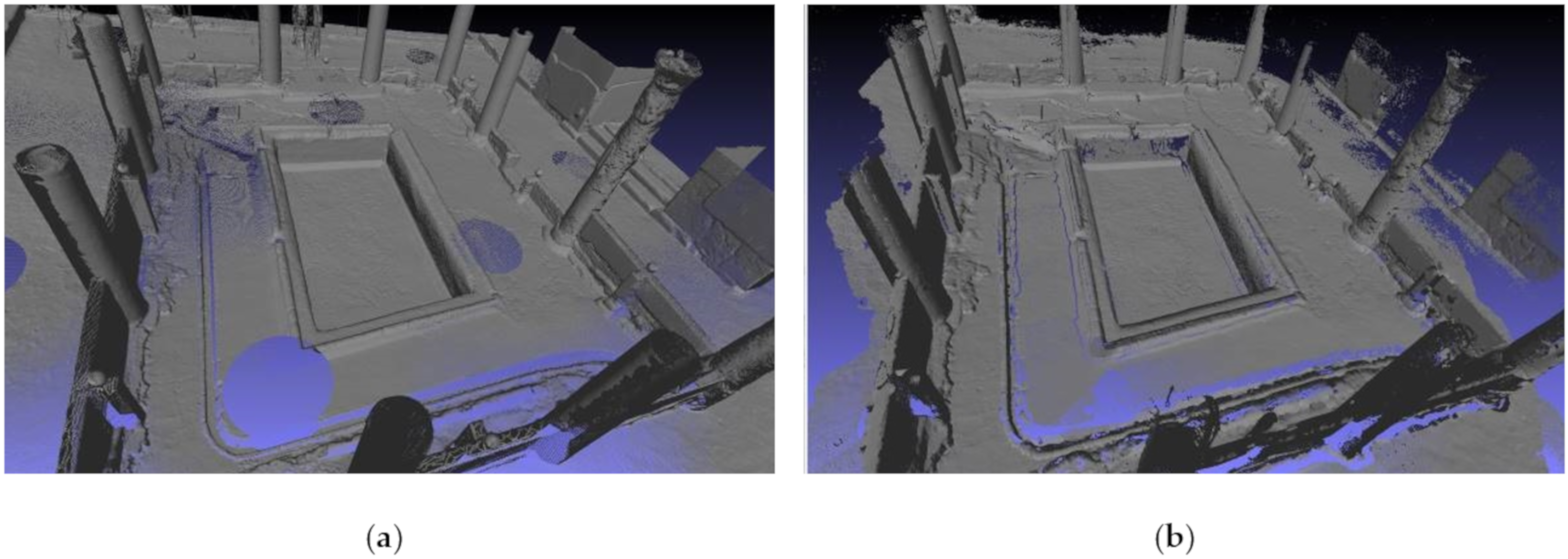
The last step is the generation of depth maps of the scene. For this, we start with a main image and eight adjacent secondary images, according to the direction of data capture. Depth values are calculated for each X and Y position of the image [
49]; subsequently, all the generated point clouds are merged together, aligning them in a general co-ordinate system (
Figure 4a).
2.4.1. Point Cloud Filtering
When collecting data from the prototype, it is typical that the obtained point clouds have noise and artifacts that must be removed. In reality, these are outliers, which can be numerically separated from the rest and which must be eliminated (
Figure 4b). In our case, we applied two filters [
51,
52]: (1) First, a statistical outlier removal (SOR) filter, which analyzes a set of n points by calculating the average distance between them; any point that is more than σ standard deviation from the mean distance is detected as an outlier and removed (in our case, the values used for n and σ were 200 and 0.8, respectively); (2) subsequently, a radius outlier removal (ROR) filter is applied, with which a set of k points is fitted to a local plane, following which the normal of the plane through the points is computed and the radius (R) of a virtual sphere is defined, which is used to count the excess neighbors. As a result, the points outside of this sphere are detected as outliers and removed—only those points closest to the adjusted plane and that best define the object are kept.
2.4.2. Mesh and Texture Mapping Generation
Once the point clouds and depth maps have been generated (as in
Section 2.4), an algorithm to eliminate distortions [
53] is applied to the selected images, using the camera calibration parameters obtained in
Section 2.1. Subsequently, to carry out the texture mapping, the Poisson algorithm [
54] is used, in which a mesh formed by a series of triangles adapted to the point cloud is generated (see
Figure 4c). Taking into account the position of the camera’s projection center, the size and position of the triangle, and the orientation of its normal vector, each triangle will be associated with one or more main images corrected for distortions (with their original color) [
55]. To transfer the generated textures to the point cloud, a two-step procedure [
55,
56] is carried out: First, an algorithm that transfers the color of the texture projecting it onto the vertices of the mesh is used; then, the colors of the vertices are transferred to the point cloud, following the criterion of associating the color of the vertex with the closest points (
Figure 4c); the result will be optimal if the average length of the sides of the triangles of the mesh coincides with the distance between points of the point cloud; otherwise, a loss of resolution may be observed in the projected texture.
3. Experimental Test
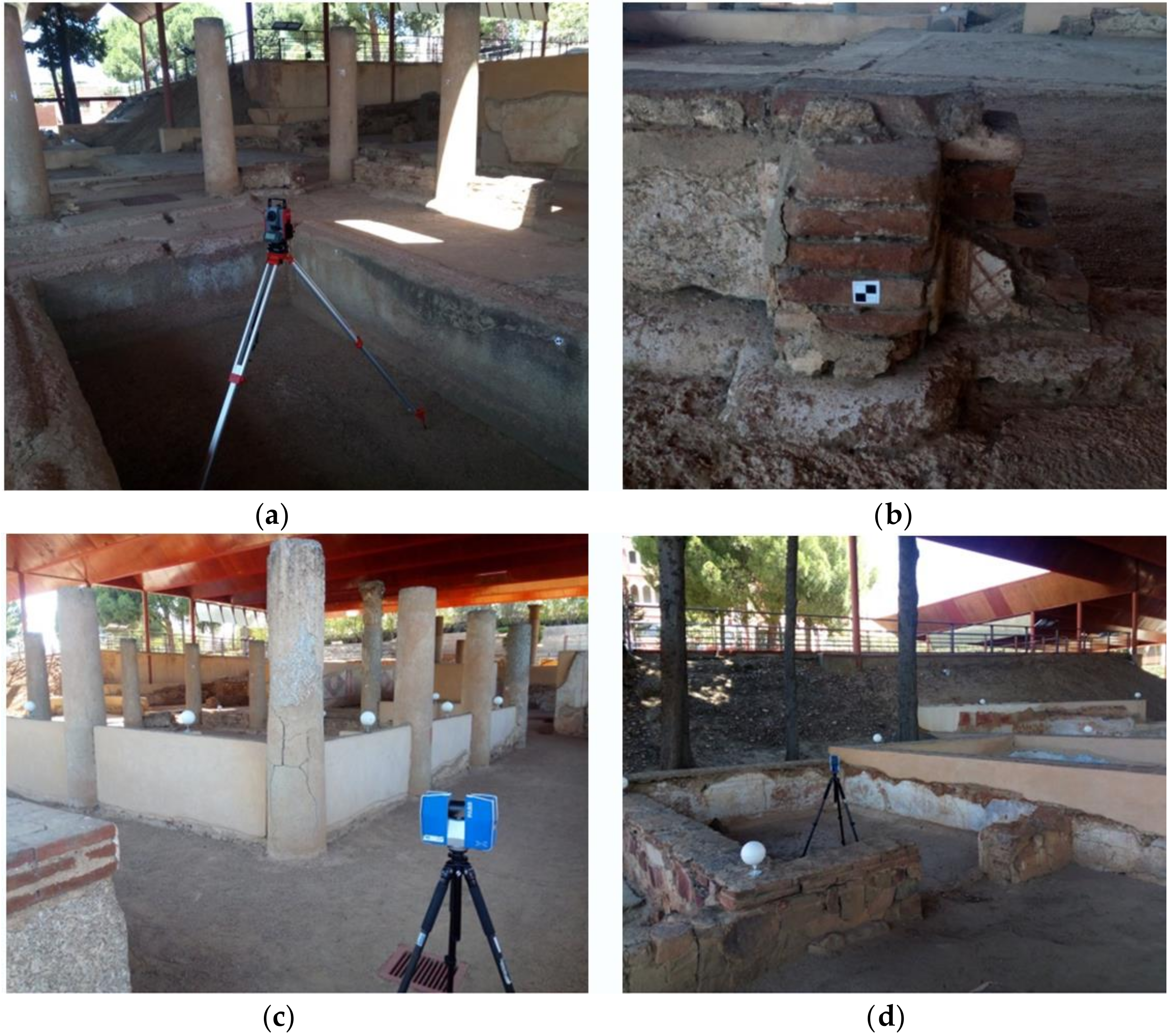
To evaluate the effectiveness of the system proposed in this paper, a set of various studies were performed in the House of Mitreo (Mérida, Spain), a dwelling from Roman times built between the first century BC and the seocnd century AD. Within this archaeological set, three working areas were chosen, due to their own characteristics, in which different aspects of the proposed system were tested:
Working area 1: Pond and peristilium. In this area, it was intended to observe the behavior of the device in areas with different height levels and horizontal and vertical construction elements, as the area consists of a water tank (currently empty) located below the ground, and columns that rise up to 2.5 m above the ground (
Figure 5a). One aspect to be evaluated was the behavior of the device in capturing the columns due to their geometry, which can pose a challenge for the calculation of homologous points and subsequent relative orientations. Another aspect to evaluate was that, as the data collection required two different trajectories—one inside the pond courtyard and the other outside (through the peristilium)—we checked if the system adjusted both trajectories properly and whether the drift error was acceptable.
Working area 2: Underground rooms. This part of the house was used in the summer season. Being excavated below ground level, there was a lower temperature inside than in the upper area. These are accessed through a staircase with a narrow corridor, surrounded by high walls and with remains of paintings and notable differences in lighting between the lower and upper parts (
Figure 5b). It was, therefore, an interesting area to study the behavior of the proposed system in narrow areas, as well as the adaptability of the system to different lighting levels and complex trajectories.
Working area 3: Rooms with mosaic floors (
Figure 5c). Mosaics are typically repetitive geometric figures materialized by a multitude of small tiles. Thus, their 3D reconstruction could pose a challenge for the proposed system, leading to errors in matching homologous points causing gross errors or even the impossibility of orienting the images. Regarding data capture, work in this area requires long and complex trajectories, in order to cover all areas without accumulating drift errors. In addition, the small size of the tiles that make up the mosaic floors and their different colors demand a high capacity in the resolution and definition of the captured textures.
To carry out validation of the proposed system, the same work areas were scanned, in addition to the proposed system, by a Faro Focus3D X 330 laser scanner, with a range of 0.6–330 m, a scanning speed of 976,000 points/seg, and a maximum precision, according to the manufacturer, of 1 mm @ 5 m. In addition, to perform a metric control of both systems, a total of 150 targets were placed throughout the three areas. Their co-ordinates were measured by the total station Pentax V-227N (Pentax Ricoh Imaging Company, Ltd., Tokyo, Japan) with an angular precision of 7″ and 3 mm + 2 ppm of error in distance measurement (ISO 17123-3: 2001) (
Figure 6).
With these data, we carried out a set of tests in which both systems (i.e., the proposed system and the laser scanner) were evaluated and compared:
The first test compared the time spent in data acquisition and data processing.
In the second test, a series of calculations and experiments were performed to determine the resolution and distribution of the point cloud of both systems in a comparative way.
The third test evaluated the precision of both systems through three different sub-tests. In the first sub-test, 150 targets were measured as control points and a comparative study was carried out on the accuracy assessment of both systems; in the second sub-test, precision and zonal deformations were evaluated, in which the presence of systematic errors between the proposed system and the laser scanner were ruled out by means of circular statistical analysis. In the third sub-test, a visual comparison was made between cross-sections of the point clouds resulting from both systems.
The last test evaluated the resulting textures of both systems through the analysis of different variables.
The tests mentioned above are described in detail below.
3.1. Comparison Times for Data Acquisition and Processing
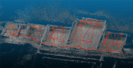
Data acquisition with the proposed system consists of focusing the device towards the area to be measured and moving along a trajectory which the VSLAM algorithm continuously calculates, the graph of which appears in real time on the laptop screen; in this way, the user can ensure that there is continuity in the capture and that the system is not interrupted (
Figure 7). The distances between the measured elements and the device varied from 0.4 to 2 m in working areas 1, 2, and 3; likewise, the parameters that defined the resolution were not chosen until the post-processing phase and did not determine the times used for data acquisition.
For data collection with the Faro Focus X 330 laser scanner, a resolution of ½ of the total was chosen among the configuration parameters, along with a quality of 4x, which, according to the manufacturer’s data [
19], achieves a resolution of 3.06 mm @ 10 m distance. Furthermore, the scanner took 360 images at each scanning station. In the methodology used, different positioning of the instrument was necessary to avoid occluded areas.
Regarding the subsequent phase of data processing, the proposed system acts autonomously; that is, practically without user intervention, where the user only has to choose some initial parameters when starting the process. However, the laser scanner’s post-processing work required more operator intervention or, in some cases, the performance of operations that require a high time cost, such as the scan loading process, which may takes several minutes, registration of the reference spheres, which must be supervised manually, the assignment of colors to the scans, and so on. The results can be seen in
Table 2, where the times used by each system in different areas are shown, both for data collection and data processing. Regarding the results obtained, the time required for data acquisition with the proposed system was 31 min (0.52 h) in total for the three working areas, compared to 520 min (8.67 h) with the Faro Focus3D X 330 laser scanner; that is, the proposed system was about 17 times faster in capturing data than the laser scanner. The preliminary work of the laser scanner, the placement of reference spheres, and the necessary station changes were also considered in this time measurement. However, in data processing (CPU time), the laser scanner system was about 10 times faster than the proposed system: 176 min (2.93 h) for the former, compared to 1716 min (28.60 h) for the latter. However, it should be noted that the user spent a total of 97 min (1.62 h) in the data processing operations with the laser scanner system but, with the proposed system, the user’s time-cost was nil, as the processing is done fully automatically.
3.2. Points Cloud Resolution and Distribution
The point clouds generated by both systems had a non-uniform point-to-point separation, where the magnitude depended mainly on the capture distance between the device and the scanned area. In order to estimate an optimal value of this parameter, the average resolution values in the three study areas were calculated. For this, the minimum distances between all points of the cloud was obtained and their average value was calculated. However, in some cases, the mean density values may have been distorted; for example, if the point clouds were obtained by merging multiple point clouds. Therefore, in order to have an independent value that confirmed the previous results, a test was carried out with the proposed system on a flat 1 m
2 surface, following movement in a direction perpendicular to the optical axis of the main image (at 1 m distance). The outlier data were removed and the resulting points were projected onto the plane; with these points, we calculated the average resolution value, as was done in the first case. The results with the resolution values of each technique are shown in
Table 3, in which the resolution obtained with the laser scanner in all cases was about 3.5 times higher than that obtained with the proposed system.
3.3. Accuracy Assessments
Evaluation of the precision of both systems was carried out through the precise measurement of 150 control targets in both systems. At the same time, detailed calculation of a control area was carried out through circular statistics and, finally, the results were obtained of a series of comparative cloud cross-sections resulting from both systems.
Figure 8 shows the results of the point clouds of both systems for the three work areas.
3.3.1. Control Points Accuracy Test
To assess the metric quality of the measurements, we analyzed the point clouds of each work area generated by both the proposed system and the Faro Focus3D X 330 system. For this, the coordinates of the 150 targets were used as control points, which were evenly distributed on pavement, walls, columns, baseboards, and so on. These coordinates were measured with the total station; in this way, each check point (target) had three coordinates: The coordinate obtained with the proposed system, that obtained with the laser scanner, and that with the total station. The results were compared following the method proposed by Hong, et al. [
57]:
First, the precision of both the measurements made by the proposed system and by the laser scanner system were evaluated using the Euclidean average distance error (
).
where
is the i
th check point measured by the proposed system (or the scanner laser),
is the corresponding check point acquired by the total station, and R and T are the rotation and translation parameters for the 3D Helmert transformation, respectively.
Then, the error vectors in the x, y, and z directions and the average error were computed. Finally, the root mean square error (RMSE) was calculated as
where
indicates the point transformed to the coordinate system of the total station.
The results obtained are shown in
Table 4, where it can be seen that the accuracy values are very similar between both systems, taking into account that the observation distances used with the proposed system were in the range of 0.4–2 m.
3.3.2. Analysis of Systematic Errors Using Circular Statistics
In the previous section, the metric quality of the point clouds was analyzed from the point of view in which only linear magnitudes were taken into account. However, we are obviating the possible existence of anisotropic behaviors, in which the magnitudes of error would follow a particular direction, which, in the case of the measurement instruments used (i.e., the laser scanner and proposed system), would confirm the existence of some systematic error between both systems, which should be corrected. To analyze this possibility, we resorted to circular statistics [
58,
59], designed exclusively for the analysis of directions or azimuths, whose basic descriptive statistics are as follows:
- -
Average azimuth
obtained by the vector sum of all the vectors in the sample, as calculated by the following equations:
- -
Modulus of the resulting vector (
), obtained by the following expression:
- -
Average modulus
, obtained by the following expression, where n is the number of observations:
- -
Circular variance of the sample
, which is calculated by
- -
Sample standard circular deviation
, being
Concentration parameter (κ), which measures the deviation of our distribution from a uniform circular distribution. Its values are between
(uniform distribution) and
(maximum concentration). For values of κ > 2, this parameter indicates concentration. The value of κ is calculated using the following expressions:
Likewise, to check the uniformity of the data, uniformity tests such as Rayleigh, Rao, Watson, or Kuiper [
59,
60,
61] were applied.
In our case, we carried out two data samples from both systems: One on a horizontal mosaic and another on a vertical wall with the remains of decorative paintings. In both cases, in the resulting point clouds, we identified a set of uniformly distributed common points; each set formed a data sample: Sample M1, in which points belonging to the vertices of the mosaic tiles were identified (42 points), and sample M2, consisting of points identified in the details and color changes of the paintings on the vertical wall (28 points). In both cases, we obtained their co-ordinates in each system using the CloudCompare (GPL Lisence) software.
With these data, we obtained the descriptive statistics of
Table 5 and, further, we used the Oriana v4 software (Kovach Computing Services, Anglesey, Wales) to obtaining the data in
Table 6, in which it can be observed that the values obtained for the mean modulus
were relatively low (0.13 and 0.56 for samples M1 and M2, respectively), compared to the minimum and maximum values of 0 and 1 between which it can oscillate. Therefore, we can rule out the existence of a preferred data address. Likewise, the concentration parameter (κ) presented values of 0.27 and 1.35, far from the value 2, which would indicate the concentration of data. Another indicator of vector dispersion were the high values reached by the circular standard deviations
of the samples (115.3° and 61.9°, respectively). Therefore, we are assured that, in both statistical samples, the error vectors were not grouped, they did not follow a preferential direction, and there was no unidirectionality in the data. Likewise, there was a high probability that the data were evenly distributed in M2, with a lower probability in M1. In
Figure 9, the modules and azimuths referring to a common origin are represented to evaluate both their orientation and their importance. From the above, it follows that we can reject the existence of systematic errors between both systems.
3.3.3. Cross-Sections
To complete the precision analysis of the proposed system, and for comparison with the laser scanner, horizontal sections were taken from the point clouds obtained with both systems in work zones 1 and 3. The section was formed by using a horizontal plane parallel to the horizontal reference plane at a height of 0.50 m from the ground and with a thickness of 2 cm. If we superimpose both sections, we obtain the results of
Figure 10, in which the points in red correspond to the section of the cloud taken with the laser scanner and those in green to that of the proposed system, observing that they are practically coincident.
3.4. Points Color Evaluation
We compared the quality and resolution of the color in both capture systems visually, with similar lighting conditions. To analyze the color of the point clouds of both systems, the resolution of the clouds must be considered, as a noticeable decrease in the resolution of one cloud with respect to another would indicate a loss of detail in textures. In parallel, the different characteristics of the images of each system must be also considered (
Table 7); as well as the resolution of the cameras of both systems, as the capture distances were different in each system (maximum of 5 m and 2 m, respectively). Furthermore, in order to carry out an evaluation in comparative terms, the ground sample data (GSD) [
44] of both systems was calculated at the same distance of 1.5 m: The GSD of the LS camera was 0.46 mm and the GSD of the videogrammetric system was 0.57 mm (see
Table 7). Given that the difference in GSD was sub-millimeter and that the resolution of both systems was high enough, despite their differences, it can be seen in
Figure 11 that there were no significant differences in the results obtained in work areas 2 and 3.
4. Conclusions
In this article, we present a new data acquisition and 3D reconstruction device, which was evaluated and compared with the laser scanner Faro Focus3D X 330 in three case studies within the archaeological site Casa del Mitreo in Mérida, Spain.
The videogrammetric prototype that we evaluated in this paper represents an innovation, given that it is one of the first videogrammetric systems whose results are comparable to other professional capture systems. The image selection system, based on a 3D-based methodology according to Mur-Artal et al. (2017), allows for the choice of keyframes, which are more adjusted to photogrammetric needs Remondino et al. (2017). Furthermore, the filters that are applied and the generation of segments increase ostensibly the guarantee of success and precision of the procedure. Thanks to this smart and adaptable algorithm, longer and more complex captures can be scanned without orientation errors or areas without enough overlap, which hinder the relative orientation process of the images. This is an important innovation in this area, in our opinion.
In this article, we demonstrate the effectiveness of the prototype, comparing it with a laser scanner in three complex case studies. The capture times, in the case of videogrammetry, were 11, 8, and 12 min for case studies I, II, and II, respectively, which highlights the complexity and length of the trajectories (see
Figure 7). We observe that the capture times of the videogrammetric system demonstrated a significant improvement over the scanner laser in a substantial way, being about 17 times faster on average. It also improves on the amount time a user needs to spend in post-processing the data, as the videogrammetric post-processing system is fully automatic. However, the processing time without human intervention is notably higher in the videogrammetric system than in the laser scanner, with processing performed by the LS being 10 times faster.
One of the most notable results of the experimental test is that the precision of both systems are very similar, yielding good precision on the measured targets and on the intermediate data reflected in the circular statistics, whose vectors did not show any significant deformation. The same applies to cross-sections and textures, the results of which were visually similar.
The videogrammetric prototype presented here is, therefore, proposed as a professional capture system with exceptional rapidity of capture and high precision for short capture ranges. Likewise, it can be used in connection with other orientation and 3D reconstruction algorithms, thus expanding its potential.
For future work, we will focus our efforts on reducing the processing time, as well as increasing the completeness of the data, trying to guide and assist users in the field to ensure that they have scanned the entire desired area, avoiding forgotten areas. Also, a new error analysis can be implemented to obtain a better understanding of the photogrammetric survey uncertainties, according to James M.R. et al. (2017) [
62].
The videogrammetric method with high-resolution cameras here presented opens new opportunities for automatic 3D reconstruction (e.g., using drones), especially considering the need for quick capture and without prior flight planning; for example, in emergencies. Furthermore, it may be considered as complementary to MMS systems, where it can be used as a unique 3D reconstruction system or to complement Lidar systems.


