Studying the Applicability of X-Band SAR Data to the Network-Scale Mapping of Pavement Roughness on US Roads

Abstract

The traveling public judges the quality of a road mostly by its roughness and/or ride quality. Hence, mapping, monitoring, and maintaining adequate pavement smoothness is of high importance to State Departments of Transportation in the US. Current methods rely mostly on in situ measurements and are, therefore, time consuming and costly when applied at the network scale. This paper studies the applicability of satellite radar remote sensing data, specifically, high-resolution Synthetic Aperture Radar (SAR) data acquired at X-band, to the network-wide mapping of pavement roughness of roads in the US. Based on a comparison of high-resolution X-band Cosmo-SkyMed images with road roughness data in the form of International Roughness Index (IRI) measurements, we found that X-band radar brightness generally increases when pavement roughness worsens. Based on these findings, we developed and inverted a model to distinguish well maintained road segments from segments in need of repair. Over test sites in Augusta County, VA, we found that our classification scheme reaches an overall accuracy of 92.6%. This study illustrates the capacity of X-band SAR for pavement roughness mapping and suggests that incorporating SAR into DOT operations could be beneficial.

1. Introduction

One of the primary operating characteristics of a road, whether paved or unpaved, is the level of service that it provides to its users. The variation of this level of service over time provides a measure of the road’s performance. Since the 1960s, it has been shown that pavement smoothness is one of the main factors when it comes to rating the nation’s highways [1,2]. It is not only indicative of how comfortable the road is to drive on, but also affects fuel efficiency, vehicle emissions, and vehicle wear. Hence, periodic monitoring of pavement smoothness is of high importance to State Departments of Transportation in the US, as it provides input to a pavement management system.

Pavement smoothness is typically quantified through a parameter called the International Roughness Index (IRI). The IRI was developed by the World Bank in the mid-1980s as a standardized way to measure the roughness of a road [3]. It is expressed as the amount of vertical displacement per length of horizontal travel. The IRI value results from a mathematical simulation of vehicular response to the longitudinal surface profile using the ‘Golden Car’ model traveling at 80 km/h [4]. It summarizes the roughness qualities that impact vehicle response and provides a measure of ride quality. The IRI is normally reported in meters/kilometer or inches/mile.

In the US, the IRI is used for system performance monitoring and for construction acceptance. Typically, there is a target value of roughness and, hence, IRI that cannot be exceeded. For example, the Virginia Department of Transportation (VDOT) considers IRI < 140 as sufficient for Interstates and Primaries and IRI < 220 as sufficient for secondary roads. The federal government in the US has also used the IRI criterion for assessing road performance. Hence, the Federal Highway Administration has required states to measure IRI on the National Highway System every year since 1993, with the results of these measurement campaigns reported to Congress.

Remote sensing offers an alternative approach for IRI assessment that, if successful, could complement traditional measurement techniques to reduce costs. Past attempts of retrieving IRI from remote sensing have largely focused on visual remote sensing data and have predominantly shown limited IRI mapping performance [5,6]. Only one study has been published so far that investigated the suitability of SAR sensors for road roughness mapping [7]. In this past study, L-band SAR data from the Japan Aerospace Exploration Agency’s ALOS PALSAR sensor [8] was found to carry information on the roughness of high-IRI roads in Ayutthaya province, Thailand. While the IRI values encountered in Thailand are not representative for most US road networks, these initial successful results indicated the potential of SAR as an IRI mapping tool.

The research presented in this paper is adding to the existing literature by assessing the performance of SAR for mapping IRI conditions on roads typical for the United States. Specifically, we analyzed the applicability of high-resolution Synthetic Aperture Radar (SAR) data acquired at X-band frequencies to the network-wide mapping of pavement roughness of roads in the US. The X-band wavelength (~3.1 cm) was chosen due to its increased sensitivity to the small-scale surface roughness typically found on well-maintained US roads. Based on a comparison of high-resolution X-band images from the Cosmo-SkyMed satellites with road roughness data in the form of International Roughness Index measurements, a model was developed that allows estimating IRI properties and road quality information from calibrated X-band radar brightness values. Performance parameters were derived describing the IRI mapping capabilities of SAR and recommendations were formulated based on these parameters.

After introducing our study area (Section 2), we provide an overview of the SAR and reference data used in this study (Section 3). Section 4 presents the results of an initial data survey that was used to assess the general applicability of X-band SAR for this task. Our approach for developing an IRI mapping model is described in Section 5, while SAR-based IRI mapping results as well as a performance assessment of the developed technique are shown in Section 6. A discussion of the potential role of SAR in pavement roughness mapping (Section 7) and a summary of our work (Section 8) conclude the paper.

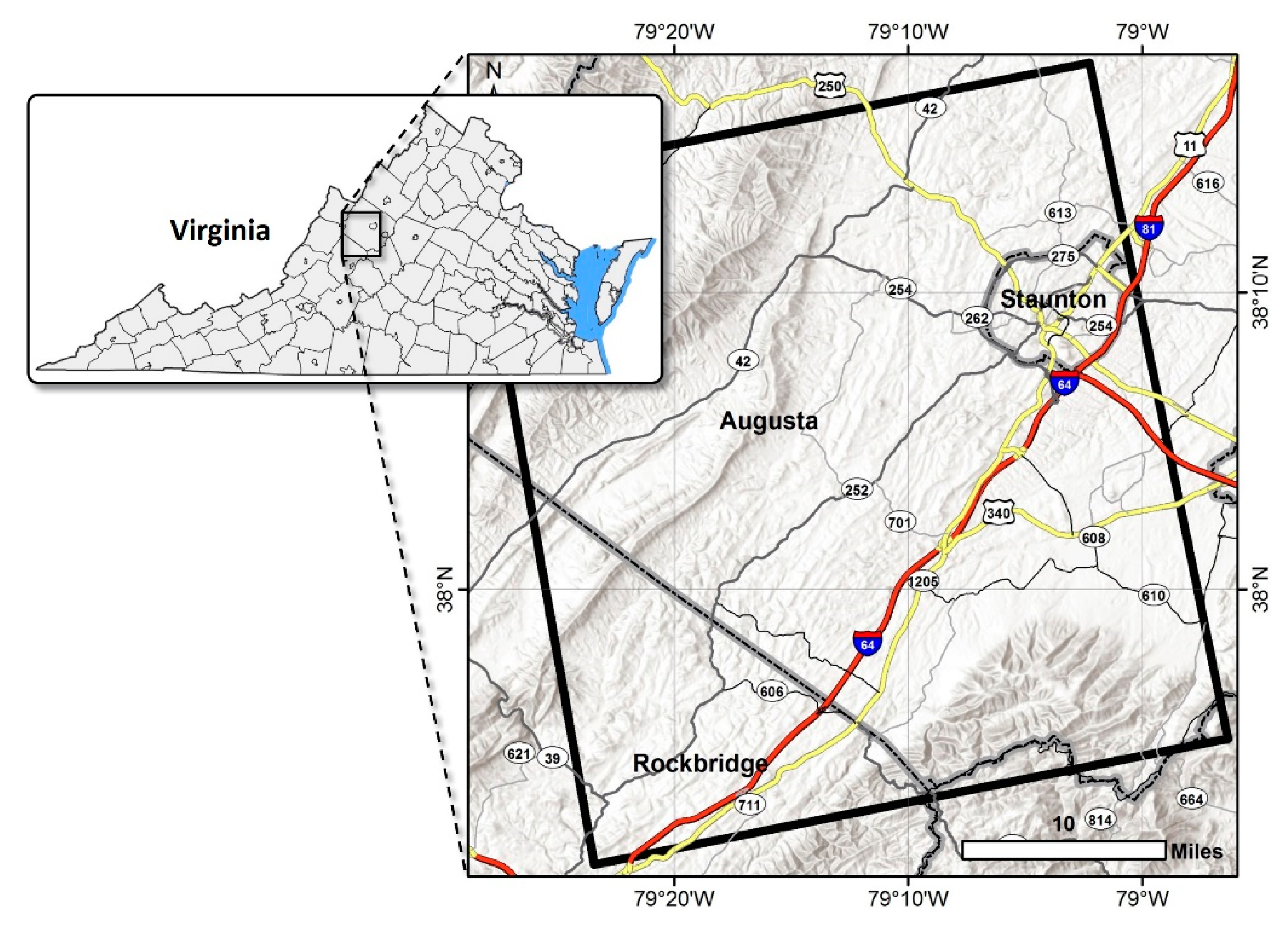
2. Area of Interest

Our study is focused on Augusta County, VA, the second largest county by total area in the Commonwealth of Virginia (Figure 1). Augusta County is embedded within the Shenandoah Valley and surrounds the independent cities of Staunton and Waynesboro. As of 2019, the county had a population of 75,558 with an average population density of 76/mi² [9]. The county’s people reside in near 30,000 households spread through two major towns and an additional 14 unincorporated communities. Augusta County has a maintenance jurisdiction for more than 1330 miles of road, with most belonging to the category of local secondary roads [10].

The Augusta County area was selected for this study as it contains a wide variety of interstate, primary, and secondary roads. It is representative of typical US rural settings in terms of housing structure, geographic setting, and economic activity [11]. Its population density is representative of the US counties east of the Mississippi River [9]. Therefore, Augusta County is a suitable site to evaluate SAR-based IRI mapping methods under representative conditions.

The road characteristics in our study area are typical for roads across the United States. In the Augusta County and throughout Virginia, interstate highways are federally mandated to have a 12-feet (3.65 m) lane width. The overall pavement width of interstates depends on the number of lanes but exceeds 24 feet throughout our area of interest. The width of primary roads in Augusta County varies depending on traffic volume, speed rating, and rural/urban classification, but in general, individual lane widths are between 11 and 12 feet (3.35–3.65 m per lane). Secondary roads in our area of interest have lane widths ranging from 9 to 12 feet (2.74–3.65 m) depending on the location and traffic volume [12]. In general, a typical two-lane secondary road in Augusta County has an overall pavement width ranging from 18 to 24 feet (5.49–7.32 m).

To assess pavement quality of Augusta County roads, the Virginia Department of Transportation, as many other state DOTs, conducts annual pavement condition surveys using a sensor-equipped vehicle. Due to the significant total road length in the county, only a small part of the county’s roads can be assessed every year. Typically, VDOT maps all interstate and primary roads and only approximately 20% of the secondary road system each year. For instance, in 2012 the VDOT obtained IRI measurements along a total of 430 road miles (23% of total road length) while IRI data from 2014 covers 475 miles (26% of total road length). This indicates the level of effort involved in maintaining pavement condition data on a network scale.

Within Augusta County, we centered our research mostly on a segment roughly 1500 mi² in size that is encompassing the city of Staunton and is shown in Figure 1. This area was picked due to the broad diversity of road types with widely varying pavement conditions that are found in this region.

3. Remote Sensing and Ancillary Data Used in This Study

3.1. Remote Sensing Data

To ensure sensitivity to the typically low level of roughness on US roads and to guarantee sufficient spatial resolution for interstates as well as primary and secondary roads, we based our study on 3 × 3 m-resolution Stripmap-type X-band SAR data from the Cosmo-SkyMed (CSK) constellation [13]. The X-band wavelength (~3.1 cm) used by CKS provides sensitivity to cm—scale surface roughness and was deemed the most suitable of all SAR wavelengths for studying US pavement roughness. The 3 m resolution is a good compromise between spatial coverage and spatial resolution. Data were acquired in VV polarization due to the higher sensitivity of VV to roughness scattering [14]. Finally, the 16-day revisit time of the CSK satellites provides excellent temporal sampling of pavement conditions in our area of interest.

Sixty-two CSK images were ordered and acquired between 29 August, 2011 and 24 November, 2014 to support this research (see

Table 1. Information regarding the SAR data used in this study.

Radar Data Information
SAR Sensor Constellation	Cosmo-SkyMed (CSK)
Spatial Resolution	3 × 3 m
Signal Polarization	VV
Line-of-Sight Off-Nadir Angle	24.23°
Orbit Direction	Ascending
Track	213
Revisit Frequency	16 days
Time Period Covered by Data	29 August 2011–24 November 2014
Number of Processed Images	62

for more information regarding the radar imagery). The good temporal sampling of our area of interest increased the likelihood of near-simultaneous SAR and IRI data collected. Ascending-mode data of track 213 were used, providing good coverage of our area of interest (see the black outline in Figure 1).

While the CSK data were available as complex products, carrying both amplitude and phase information, our study focused on the use of amplitude data only. This choice was motivated by our strong belief that SAR backscatter information carries relevant yet typically untapped potential in transportation infrastructure monitoring. Additionally, amplitude analysis requires less specialty knowledge about the SAR image formation process and is, hence, easer to conduct by an end-user such as a State DOT.

3.2. Road Pavement Roughness Data

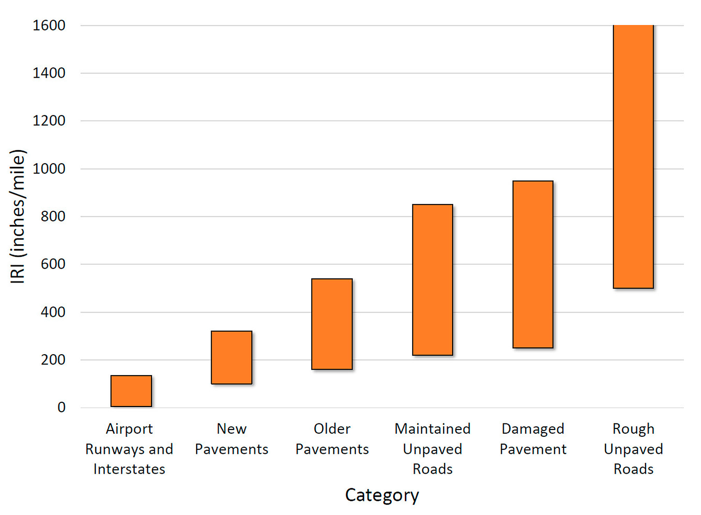
To study the relationship of SAR image brightness values to pavement conditions on US roads, we collected road roughness data for a large subset of roads within the area covered by the CSK SAR image frames (Figure 1). Roughness information was available to the research team through the services of our colleagues at the VDOT and were provided as IRI data points. Figure 2 shows the IRI roughness scale range as replotted by [15]. The lowest value of the IRI is 0 for a perfectly smooth road and as road roughness worsens, the IRI values increase. The unit of the IRI used in this study is inches/mile. Moreover, plotted in Figure 2 are the various road types and road qualities that are typically associated with a specific IRI value range. It can be seen that there is a strong overlap between the IRI ranges for different road types. Hence, the Virginia Department of Transportation uses different IRI thresholds to identify road segments in need of repair for different road categories. An IRI < 140 is considered sufficient for Interstates and Primaries, while IRI < 220 is applied for secondary roads.

The IRI data available for this study stem from two road surveys that were conducted in Augusta County in 2012 and 2014. These sampling times overlap well with the temporal coverage of the CSK SAR imagery (Table 1). While SAR data were acquired throughout the year, we are focusing here on SAR imagery that was collected near the acquisition times of our IRI field measurements to perform a valid comparison of the two data sets.

Out of the 2012 and 2014 surveys, we identified a total of 1176 IRI measurement points that were suitable for comparison with SAR observations. IRI samples were available for interstates and secondary roads in Augusta County (data on primary roads were not collected during the 2012 and 2014 IRI surveys). The IRI measurements available for this study correspond to average values derived along 0.1-mile road segments. Therefore, they are representative of the average pavement conditions over this 0.1-mile stretch. On interstates, separate IRI measurements were available per road direction while the narrower secondary roads were represented by only one measurement per road segment.

To provide an independent means for validating a developed IRI mapping algorithm, the available IRI points were separated into a training and a validation set through a random selection process. The random selection was carried out separately for interstate and secondary roads and resulted in equally-sized training and validation sets for both road types.

4. Initial Assessment of the Relationship between IRI and X-Band Radar Brightness Data

Before conducting a more sophisticated analysis of the correlation between IRI and SAR data, we performed an initial data survey to evaluate if there is any measurable relationship between IRI and X-band radar brightness measurements. For this initial analysis, SAR data were radiometrically calibrated using published calibration factors [16], geocoded, and scaled into a ${\sigma }^0$ linear amplitude scale. In a GIS system, calibrated SAR images were overlain with road centerline data and radar brightness information was extracted separately along interstates and secondary roads. IRI points were similarly associated with their respective road types.

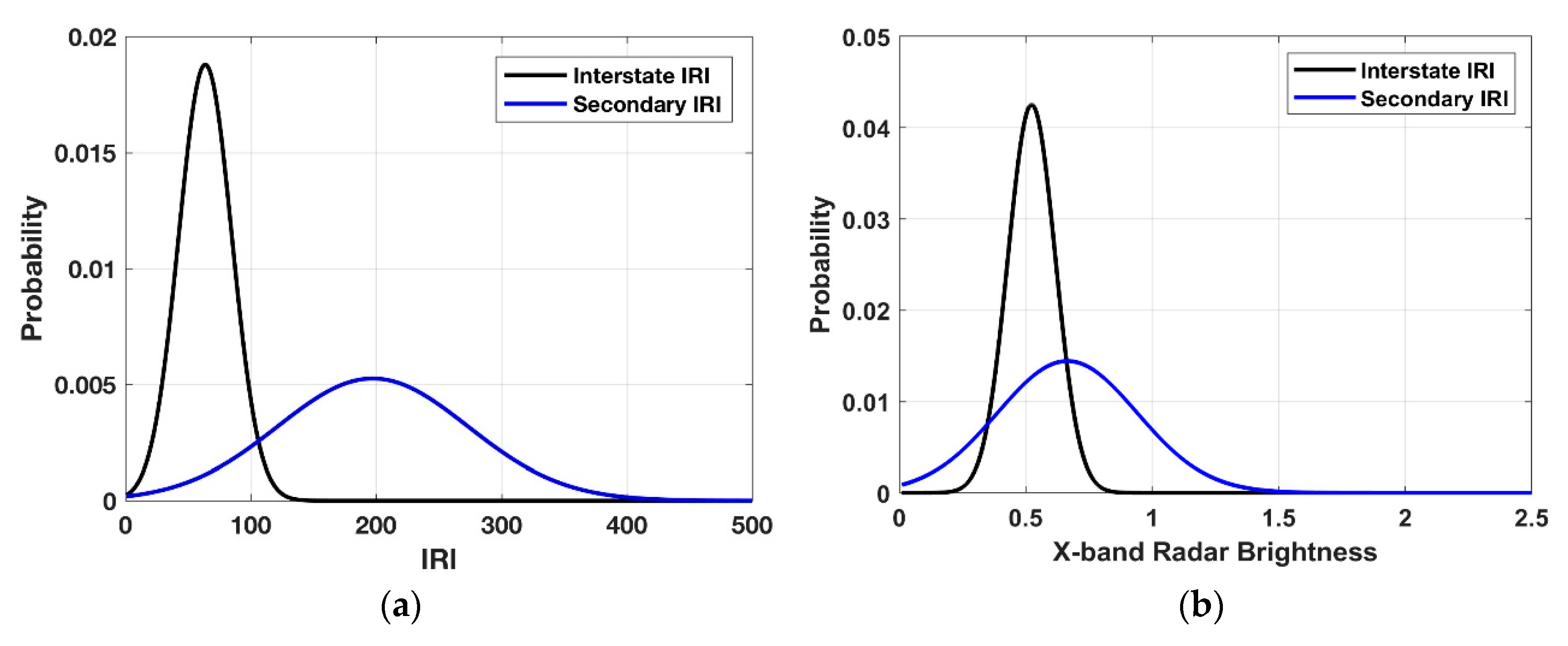
Both the collected ${\sigma }^0$ and IRI data were analyzed statistically and their probability density functions are shown in Figure 3a,b, respectively, as a function of road type. The IRI data in Figure 3a show that the pavement roughness on interstates (black line) and secondary roads (blue) is distinctly different, with lower IRI values associated with interstates compared to secondary roads. This result is commensurate with the higher maintenance requirements for interstate roads. The relative shape of the distributions also indicates that IRI data on interstates have lower variance than the data points on secondary roads. This suggests that the road quality on interstates is more consistent across the analyzed road network. Figure 3b shows that this behavior is closely mirrored in the X-band radar brightness data. Interstates are generally associated with lower and more consistent radar brightness values. While the separation between the analyzed road types is less distinct in the SAR data, IRI and radar brightness values seem to exhibit similar trends, indicating that X-band radar brightness information may be a useful indicator of a road’s pavement roughness.

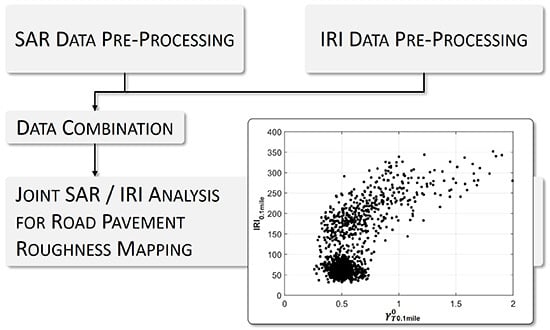
5. Developing a Forward Model for Pavement Roughness Mapping from X-Band SAR

Based on these initial encouraging findings, we aimed at developing a forward model that describes the expected correlations between IRI and X-band radar brightness data and can be used to invert high spatial-resolution IRI information from calibrated CSK SAR measurements. The workflow we used to arrive at a correlation model is shown in Figure 4. After initial preprocessing steps for both SAR and IRI data (see top left and right of Figure 4, respectively), all measurements were combined to facilitate joint data analysis and forward model development (bottom of Figure 4). The main processing steps of our workflow are briefly described in the following sub-sections.

5.1. SAR Data Preprocessing

To prepare the CSK SAR data for comparison to IRI samples, all SAR images were radiometrically calibrated to allow for a comparison of radar brightness values in repeated image data [17]. Furthermore, images underwent geometric and radiometric terrain correction before image analysis. Radiometric Terrain Correction (RTC) was applied to remove slope impacts on the road surface SAR backscatter values, which would lead to local biases of the measured radar brightness [18,19] and may impact potential relationships between SAR data and pavement roughness as parameterized by IRI. RTC processing uses terrain information to calculate the precise area a pixel occupies on the ground. This area estimate is subsequently used to normalize the calibrated radar brightness measurements, resulting in terrain-corrected gamma naught (${\gamma }_T^0$)—projected data. The RTC algorithm in [20] was used in our workflow and digital elevation models (DEMs) needed for RTC processing were extracted from the National Elevation Dataset (NED) [21]. To maximize the RTC processing performance we ensured accurate registration between the NED DEM and the SAR image stack by applying a two-step alignment procedure. First, we correct the SAR observables for bulk atmospheric path delay using atmospheric model data. Second, we generate a simulated SAR image from the DEM data and correct for residual registration issues by co-registering the SAR data stack to this simulated SAR image [22]. This two-step approach ensures the necessary alignment between the DEM and SAR image to facilitate RTC processing.

While RTC processing removes pixel area influences on SAR backscatter, there are other potential factors that may affect SAR/IRI relationships. These include (i) incidence angle dependencies of surface scattering properties as well as (ii) effects of weather events (standing water after rain events, snow, or ice on pavement) on radar brightness: A number of studies have shown that (i) backscattering properties of most rough surface scatterers (such as road pavement) change only slowly with incidence angle [23,24]. Therefore, combined with the narrow swath of the dataset used, we expect the impact of incidence angle variations on calibrated and RTC processed ${\gamma }_T^0$ values to be small. To mitigate weather impacts (ii), we screened our observations using a local weather station in Staunton, VA (station KVASTAUN37) and removed observations impacted by precipitation in proximity to the image acquisition time.

We selected linear amplitude-scaled ${\gamma }_T^0$ data as the most suitable data source for ${\gamma }_T^0$-vs-IRI modeling. Compared to power- and dB-scaled data, the amplitude option provided the best model fit with IRI field measurements.

As maintenance requirements for road roughness in the US are strict, roads are typically smooth and the X-band ${\gamma }_T^0$ values measured for US roads remain near the sensor’s noise level. Hence, high-performance suppression of speckle noise along narrow road segments is paramount for successful IRI estimation, especially if the spatial resolution of derived IRI information is a concern. As our VDOT partners were interested in optimizing along-road resolution of derived IRI parameters, within this study, we tested a range of speckle suppression methods for their applicability to filtering narrow road segments. From our analyses, we found that stack covariance-based algorithms such as the DespecKS^TM technique [25] were best suited for road surface analysis. Hence, all of the classification results shown in this paper are based on DespecKS-filtered data, which were processed and provided to the team by project partner TRE ALTAMIRA. For researchers that do not have sufficient data or compute resources for stack covariance processing, we recommend the nonlocal means filter in [26] as an alternative Speckle suppression approach. If spatial resolution is not a strong requirement, spatial averaging along the main pavement axis can be applied instead (see Section 5.3).

No additional multi-looking was applied after speckle filtering to preserve the resolution capabilities of the sensor, and data were geocoded to a ground-sampling distance of $3\times 3 \mathrm{m}$. The performance of our geocoding process benefited from the co-registration of DEM and SAR data that was performed during RTC processing. Once combined in a GIS environment, we found good alignment of SAR and road centerline data at the 3-m pixel level.

5.2. IRI Data Preprocessing

To facilitate a direct comparison with calibrated SAR ${\gamma }_T^0$ data, all available IRI points were projected into the UTM coordinate system carried by the geocoded and radiometrically terrain-corrected SAR observations. Subsequently, the IRI points were imported into a GIS system, projected onto the preprocessed SAR images and overlain with road centerline data. A geospatial comparison of road center lines and IRI data points was performed to identify and remove IRI measurements that were mislocated from the pavement surface. Occasional geometric misplacements of IRI points were largely related to spurious errors in the recorded GPS coordinates. A removal of these points was necessary as the SAR ${\gamma }_T^0$ values at the incorrect sampling locations are not representative of the IRI information measured for these points.

5.3. SAR Data Extraction at IRI Point Locations

As IRI measurements available for this study represent the average pavement conditions along 0.1-mile road segments, we compare IRI data to SAR ${\gamma }_T^0$ values averaged over the same road segment length. To this end, SAR data were overlain with road centerline data and IRI point locations, and along-road averaged ${\gamma }_T^0$ values were calculated for every 0.1-mile road segment centered on IRI data point coordinates. The resulting averaged ${\gamma }_T^0$ data (${\gamma }_T^0{}_{0.1\mathrm{mile}}$) and their respective IRI information were then stored in an ${\gamma }_T^0$ vs. IRI database, which forms the basis for the subsequent forward model development.

5.4. ${\gamma }_T^0$ vs. IRI Forward Model Development

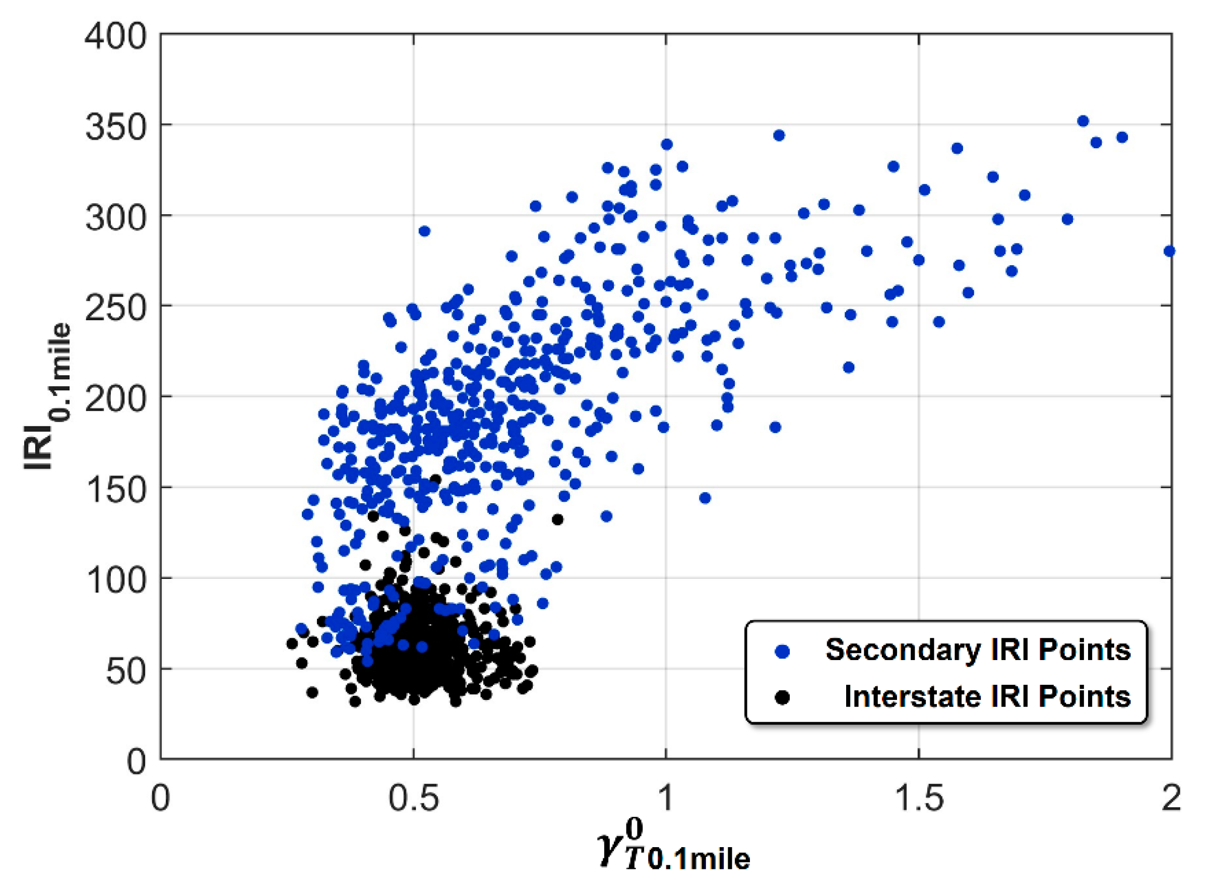
To develop a model that relates ${\gamma }_T^0{}_{0.1\mathrm{mile}}$ values to the corresponding IRI information, we extracted all samples from the generated ${\gamma }_T^0$ vs. IRI database that belong to our training set (see Section 3.2) and analyzed their information content. Figure 5 shows the relationship between IRI (y-axis) and ${\gamma }_T^0{}_{0.1\mathrm{mile}}$ values (x-axis) for the training set, indicating a measurable correlation between these data types. While ${\gamma }_T^0{}_{0.1\mathrm{mile}}$ measurements appear to be reasonably constant for IRI values between 0 and $120 \mathrm{inches}/\mathrm{mile}$, an increase of ${\gamma }_T^0{}_{0.1\mathrm{mile}}$ with IRI can be observed for IRI values beyond the $120 \mathrm{inches}/\mathrm{mile}$ threshold. This indicates that X-band SAR data may be useful to estimate road roughness above the $IRI\approx 120 \mathrm{inches}/\mathrm{mile}$ scale.

The color-coding of Figure 5 provides additional information about the ${\gamma }_T^0$ vs. IRI data correlation by analyzing the influence of different road types on the correlation pattern. Similar to Figure 3, the data points associated with interstates form a tight cluster with little variance along both the IRI and ${\gamma }_T^0$ axes. The circular shape of the interstate data cluster suggests little-to-no correlation between IRI and ${\gamma }_T^0$ for this road type. For secondary roads, however, a significant correlation of IRI and X-band ${\gamma }_T^0$ measurements can be observed.

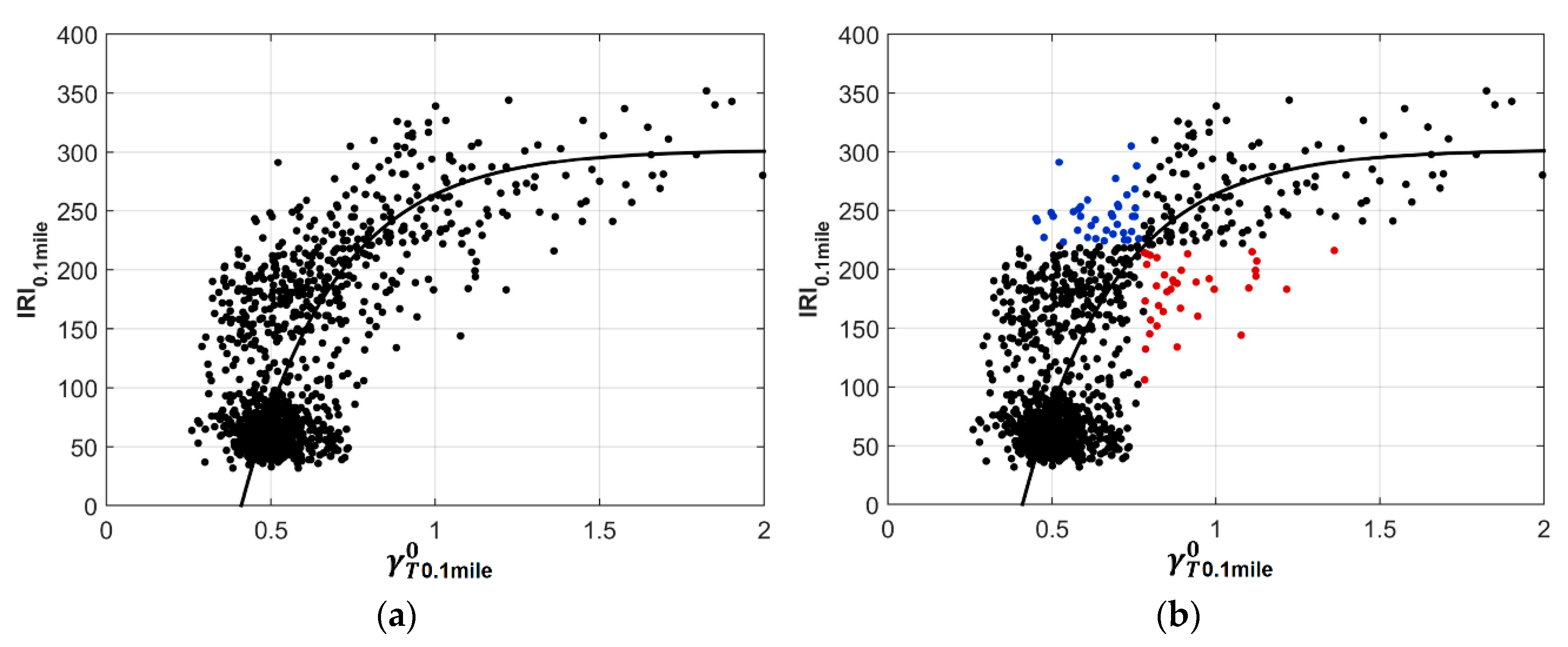
To enable road quality assessment from SAR, we developed a forward model that best describes the ${\gamma }_T^0{}_{0.1\mathrm{mile}}$ vs. IRI relationship for the full IRI range shown in Figure 5. After testing several functional models for their fit with the data, we found the best modeling performance when using an exponential model of the form.

$$IR{I}_{SAR}={\alpha }_1\times \left[1-exp\left(-{\alpha }_2\times \left({\gamma }_T^0{}_{0.1\mathrm{mile}}-{\alpha }_3\right)\right)\right]$$

(1)

Equation (1) models IRI as a function of SAR ${\gamma }_T^0$ measurements. The unknown model parameters ${\alpha }_1$, ${\alpha }_2$, and ${\alpha }_3$ define the scale, shape, and x-offset of the exponential function, respectively. The unit of ${\alpha }_1$ is [$\mathrm{inches}/\mathrm{mile}$] while ${\alpha }_2$ and ${\alpha }_3$ are unitless. We derive estimates ${\widehat{\alpha }}_1$, ${\widehat{\alpha }}_2$, and ${\widehat{\alpha }}_3$ for the model parameters via a least-squares fit of (1) relative to the data in Figure 5. The best fit was achieved for the parameter combination of ${\widehat{\alpha }}_1=302\pm 2$, ${\widehat{\alpha }}_2=3.5\pm 0.2$, and ${\widehat{\alpha }}_3=0.41\pm 0.03$, resulting in the best-fitting regression model shown as a bold black line in Figure 6a. A generally good fit of the exponential model with the data can be observed and all model parameters could be estimated with low uncertainties. We invert (1) parameterized by ${\widehat{\alpha }}_1$, ${\widehat{\alpha }}_2$, and ${\widehat{\alpha }}_3$ to provide estimates of IRI based on SAR ${\gamma }_T^0$ measurements.

6. Mapping IRI Using X-Band SAR

Due to the level of noise in the data (see Figure 5), the error bars of SAR-based IRI estimates (${\widehat{IRI}}_{SAR}$) can be large (see Section 7.2 for more details on the ${\widehat{IRI}}_{SAR}$ error model). Hence, instead of estimating the exact IRI value for every road segment, a classification of individual road segments into one of two categories—“good road quality” and “road in need of repair”—was attempted. Due to the higher sensitivity of SAR to IRI values on secondary roads, we focused our classification exercise on secondary roads.

For secondary roads, the US DOT determines a threshold of $IR{I}_{thresh}=220 \mathrm{inches}/\mathrm{mile}$ to discriminate between good road segments and segments in need of repair [15]. We adopt this threshold and classify every road segment according to:

$$IR{I}_{thresh}=\{\begin{array}{c}good road: {\widehat{IRI}}_{SAR}\le 220 \mathrm{inches}/\mathrm{mile}\\ bad road: {\widehat{IRI}}_{SAR}>220 \mathrm{inches}/\mathrm{mile}\end{array}$$

(2)

For the training set, the classification quality of the model in (1) for $IR{I}_{thresh}=220 \mathrm{inches}/\mathrm{mile}$ is shown in Figure 6b where correctly classified samples are shown in black while incorrect classifications (according to the IRI reference data) are shown in either blue (bad road segment incorrectly classified as good road; type-I error) or red (good road incorrectly classified as bad; type-II error). It can be seen that, while the majority of the data samples were classified correctly, there are some misclassifications near the decision threshold.

To provide independent and quantitative information about the classification performance, we applied our SAR-based IRI mapping approach to our set of IRI validation points. We first used the model in (1) with the measurements ${\gamma }_T^0{}_{0.1\mathrm{mile}}$ to arrive at SAR-based IRI estimates ${\widehat{IRI}}_{SAR}$ for every validation data point. Then, we compared the estimates ${\widehat{IRI}}_{SAR}$ to the threshold rule in (2) and evaluated the SAR-based classification results with available IRI ground-truth information. The confusion matrix in

Table 2. Confusion Matrix Report based on IRI validation samples. Type-I errors (false positives; FP) are highlighted in blue while type-II (false negatives; FN) are shaded in red.

		Ground Truth
		Good	Bad	Total
Classification Results	Good	967 (95.0%)	36 (22.7%)	1003
	Bad	51 (5.0%)	122 (77.3%)	173
	Total	1018	158	1176

summarizes the achieved classification performance.

In the confusion matrix in Table 2, type-I errors (false positives; FP) are highlighted by a blue background while type-II (false negatives; FN) are shaded in red. A total number of 1018 positive samples (good road condition; P) and 158 negative samples (bad road condition; N) were available for this analysis. About 95.0% of good roads (true positives; TP), and 77.3% of bad roads (true negatives; TN) were correctly classified. A false positive of $FP=22.7\%$ of bad roads were classified as good roads while a false negative of $FN=5.0\%$ of good roads were classified as bad road segments. An overall accuracy of $\left(TP+TN\right)/\left(P+N\right)=92.6\%$ was achieved.

While the overall performance of our IRI mapping approach exceeded our expectations (92.6% overall accuracy) and while the number of false negatives was found to be low (5%), a larger number of false positives has to be noted (36 FPs corresponding to 22.7%). As will be shown in more detail in Section 7.3, many of these false positive are located on one specific stretch of road, suggesting that road maintenance between the acquisition of IRI and SAR data points may be the cause of a significant portion of these apparent misclassifications. The overall good condition of the road network in Augusta County and the resulting low number of available negative (bad road quality) samples in this study may have additionally contributed to an inflated false positive rate. For more information on identified sources of misclassification, please see Section 7.3.

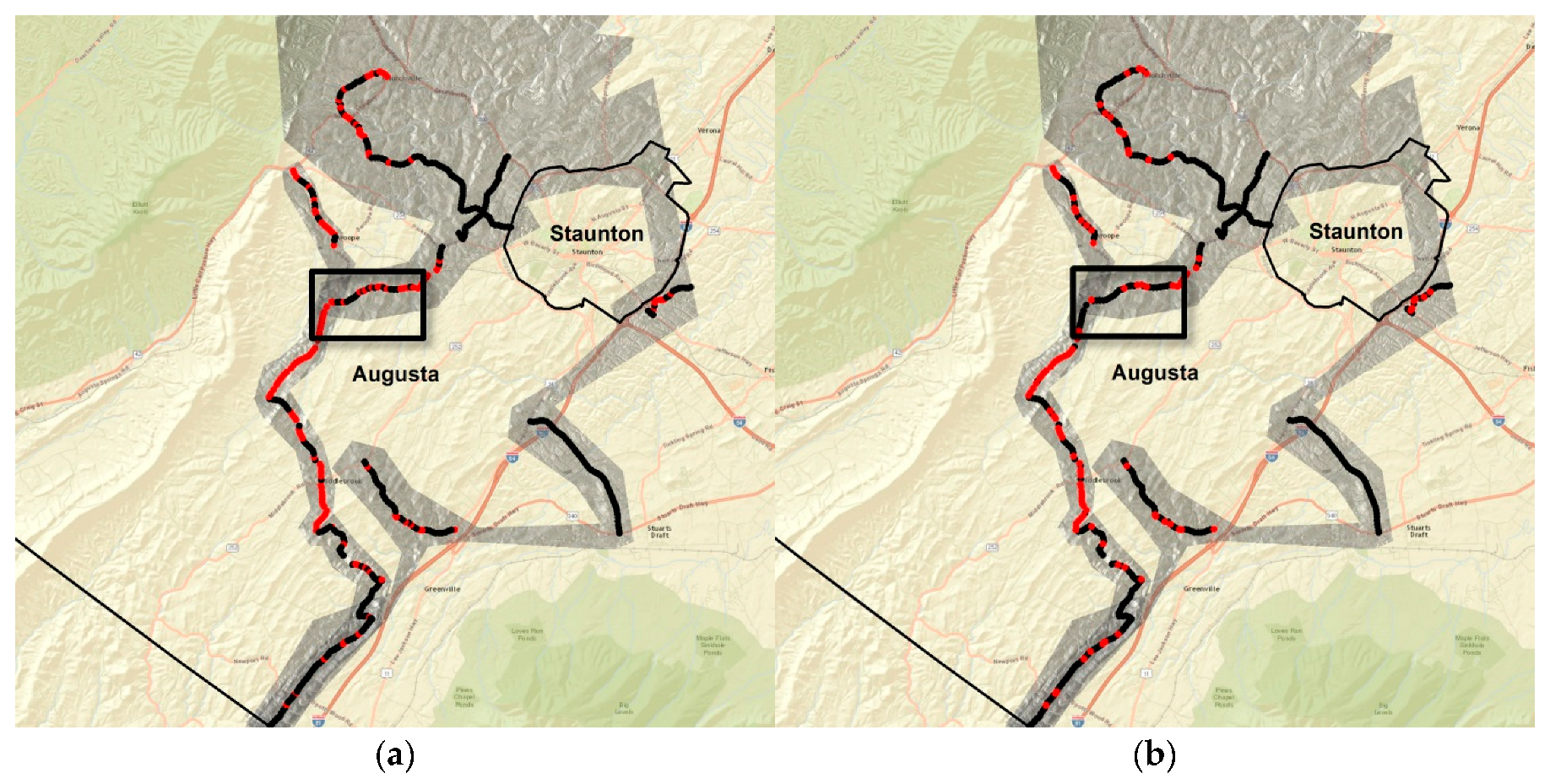
Figure 7a,b provides an example of the road classification performance by showing a map representation of both the ground-truth data (Figure 7a) and classification results (Figure 7b) for an area west of Staunton, VA. Red and black regions in Figure 7a show the distribution of bad and good road segments according to the IRI ground-truth data. Most of the low-quality road segments are concentrated on secondary roads in the vicinity and north of Middlebrook, VA. Figure 7b shows the distribution of good and bad road segments as derived from the calibrated SAR ${\gamma }_T^0$ data using Equation (1). A good match between classification results and IRI ground-truth data can be observed, indicating an overall good performance of the SAR-based classification scheme. Most road segments were classified correctly, and the spatial distribution of bad and good road segments was well preserved. The largest differences can be observed on a road west of Staunton (black rectangle in Figure 7a,b). Along this secondary road (Glebe School Road), a number of bad road segments were incorrectly classified as good roads. Reasons for these misclassifications are discussed in Section 7.3.

7. Discussion

7.1. Performance and Limitations of the Proposed ${\gamma }_T^0$ vs. IRI Signal Model

Even though several physical as well as semi-empirical models exist [14], relating surface roughness to SAR backscatter values, we chose an empirical exponential model to describe the relationship between IRI and X-band ${\gamma }_T^0{}_{0.1\mathrm{mile}}$ data. This is because IRI is only an indirect measure of pavement roughness and the relationship between IRI and pavement roughness is complicated by the involvement of the nonlinear “Golden Car model” in the IRI measurement process [27]. Hence, existing physical scattering models are not directly applicable for the task at hand.

The data distribution in Figure 5 and our choice of an exponential correlation model has implications for (i) the IRI ranges that can be mapped using this developed approach and (ii) the accuracy with which SAR-based measurements of road surface IRI can be made. Both of these implications are briefly discussed in the following sections.

The ${\gamma }_T^0{}_{0.1\mathrm{mile}}$ vs. IRI scatter plot in Figure 5 shows that for low IRI values, the capability of SAR for measuring IRI values diminishes. This is reflected by the shape of the signal model, whose steep slope at low IRI values means that a broad range of IRI values will be mapped into a narrow range of ${\gamma }_T^0{}_{0.1\mathrm{mile}}$, such that small errors in ${\gamma }_T^0{}_{0.1\mathrm{mile}}$ lead to large errors in ${\widehat{IRI}}_{SAR}$ estimates. A formal derivation of errors in ${\widehat{IRI}}_{SAR}$ is provided below.

While shallower slopes of the signal model at the high-IRI end imply better IRI estimation accuracy, it is likely that the currently selected exponential model decays too fast for high IRI. This may lead to an underestimation of errors associated with high IRI values. Furthermore, as the exponential model in (1) is asymptotic to ${\widehat{IRI}}_{SAR}={\widehat{\alpha }}_1$, IRI values larger than ${\widehat{\alpha }}_1=302 \mathrm{inches}/\mathrm{mile}$ are not represented by our model. We suggest that future research shall add more data points with $IRI>302$ to extend the current model for higher IRI (lower quality) road types.

7.2. Formal Error of X-Band SAR-Derived IRI Values

To provide quantitative information about the achievable IRI measurement accuracy, we derived a formal error model for the relationship in Equation (1). The error model in Equation (3) includes uncertainties in the estimated model variables (${\alpha }_1-{\alpha }_3$) as well as the ${\gamma }_T^0{}_{0.1\mathrm{mile}}$ measurements, and propagates them to arrive at IRI estimation errors ${\sigma }_{\widehat{IRI}}$. The following error model was applied:

$${\sigma }_{\widehat{IRI}}=\sqrt{\left(\frac{\partial IRI}{\partial {\alpha }_1}\right){\sigma }_{{\widehat{\alpha }}_1}^2+\left(\frac{\partial IRI}{\partial {\alpha }_2}\right){\sigma }_{{\widehat{\alpha }}_2}^2+\left(\frac{\partial IRI}{\partial {\alpha }_3}\right){\sigma }_{{\widehat{\alpha }}_3}^2+\left(\frac{\partial IRI}{\partial {\widehat{{\gamma }_T^0}}_{0.1\mathrm{mile}}}\right){\sigma }_{{\widehat{{\gamma }_T^0}}_{0.1\mathrm{mile}}}^2}$$

(3)

with

$$\frac{\partial IRI}{\partial {\alpha }_1}=1-exp\left(-{\widehat{\alpha }}_2\times \left({\widehat{{\gamma }_T^0}}_{0.1\mathrm{mile}}-{\widehat{\alpha }}_3\right)\right)$$

(3a)

$$\frac{\partial IRI}{\partial {\alpha }_2}={\widehat{\alpha }}_1\times exp\left(-{\widehat{\alpha }}_2\times \left({\widehat{{\gamma }_T^0}}_{0.1\mathrm{mile}}-{\widehat{\alpha }}_3\right)\right)\times \left({\widehat{{\gamma }_T^0}}_{0.1\mathrm{mile}}-{\widehat{\alpha }}_3\right)$$

(3b)

$$\frac{\partial IRI}{\partial {\alpha }_3}=-{\widehat{\alpha }}_1\times {\widehat{\alpha }}_2\times exp\left(-{\widehat{\alpha }}_2\times \left({\widehat{{\gamma }_T^0}}_{0.1\mathrm{mile}}-{\widehat{\alpha }}_3\right)\right)$$

(3c)

$$\frac{\partial IRI}{\partial {\gamma }_T^0{}_{0.1\mathrm{mile}}}={\widehat{\alpha }}_1\times {\widehat{\alpha }}_2\times exp\left(-{\widehat{\alpha }}_2\times \left({\widehat{{\gamma }_T^0}}_{0.1\mathrm{mile}}-{\widehat{\alpha }}_3\right)\right)$$

(3d)

and ${\sigma }_{{\widehat{\alpha }}_1}=2$, ${\sigma }_{{\widehat{\alpha }}_2}=0.2\mathrm{inches}/\mathrm{mile}$, ${\sigma }_{{\widehat{\alpha }}_3}=0.03$, and ${\sigma }_{{\widehat{{\gamma }_T^0}}_{0.1\mathrm{mile}}}=0.03$. The errors ${\sigma }_{{\widehat{\alpha }}_1}$, ${\sigma }_{{\widehat{\alpha }}_2}$, and ${\sigma }_{{\widehat{\alpha }}_3}$ were derived from the least-squares model fit described in Section 5.4, while ${\sigma }_{{\widehat{{\gamma }_T^0}}_{0.1\mathrm{mile}}}$ was estimated from the average dispersion of SAR amplitude data along 0.1-mile road segments.

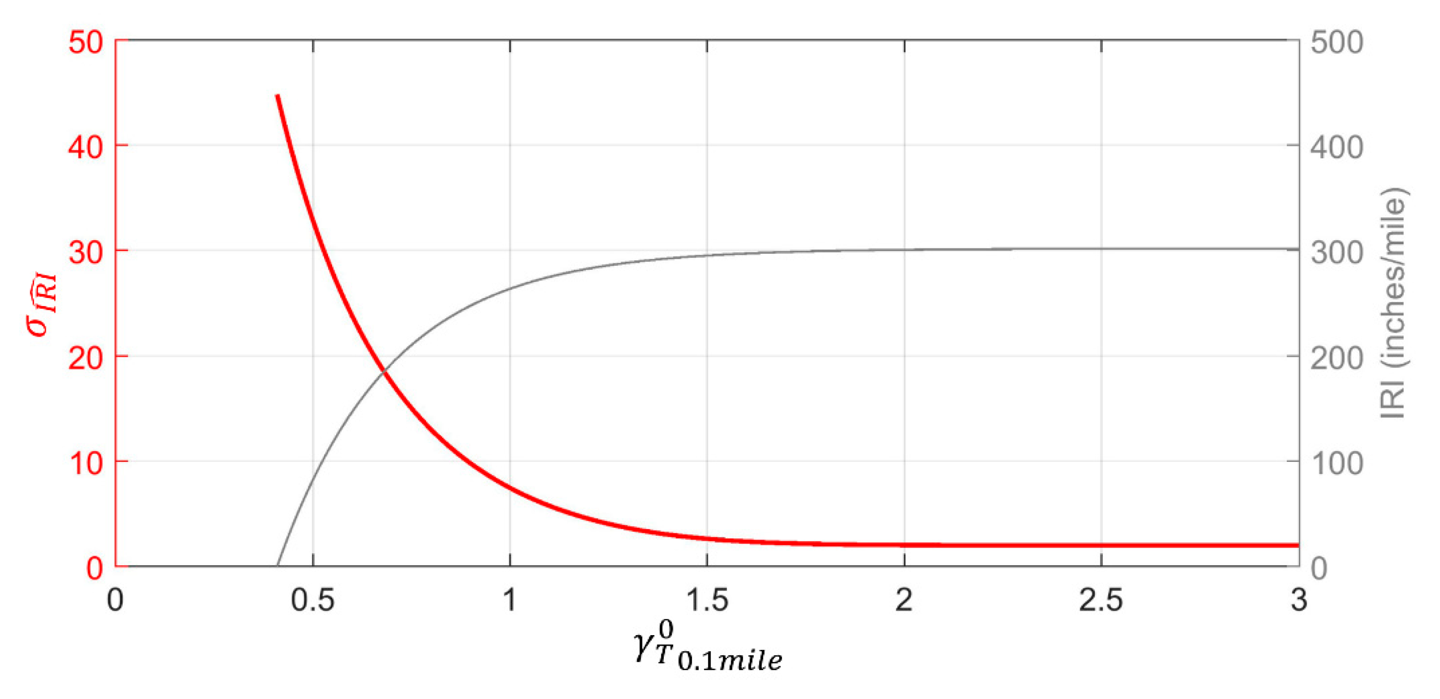
The formal errors of SAR-derived IRI values calculated according to Equation (3) are shown in Figure 8 (red line). It can be seen that errors ${\sigma }_{\widehat{IRI}}$ are large for small ${\widehat{{\gamma }_T^0}}_{0.1\mathrm{mile}}$ and, hence, for small IRI values. Errors reduce as IRI increases. Large ${\sigma }_{\widehat{IRI}}$ for low IRI values means that SAR-derived IRI estimates are not statistically different from zero for $IRI<73 \mathrm{inches}/\mathrm{mile}$ at the 95% confidence level. As 80% of interstate miles in Augusta County have IRI values below $IRI=73 \mathrm{inches}/\mathrm{mile}$, this limits the applicability of X-band SAR to mapping road quality on interstates. Decreasing estimation errors for higher IRI, however, make SAR a suitable method for mapping IRI on secondary roads.

7.3. Sources of Misclassification

Table 2 shows occurrences of both type-I and type-II errors in our area of interest. To identify the source of type-II errors, where “good quality” road segments are incorrectly classified as “road segment in need of repair”, we identified all samples affected by this error type and plotted their spatial distribution on a map for further analysis. As an example of this analysis, Figure 9a shows about four-mile long segment of VA-919, along which a significant number of type-II errors were observed. In the process of evaluating potential causes for these misclassifications, we compared type-II error locations with the presence of significant forests and tree stands (shown in green in Figure 9a) located in the direct vicinity of roads. The comparison of misclassified road segments to tree stand locations indicated that most type-II errors are due to the presence of tall trees adjacent to the road. Due to layover effects, the backscatter signature of these trees is merged with the underlying darker backscatter of the road, causing local positive ${\gamma }_T^0$ bias (brightness increase). These localized increases of ${\gamma }_T^0{}_{0.1\mathrm{mile}}$ values led to an overestimation of IRI in the affected areas. An analysis of all 51 false negatives revealed that 45 of the 51 type-II errors were found to be located in the direct vicinity of tree stands. Hence, it is likely that trees alongside roads are the main cause of type-II errors in the proposed algorithm.

Type-I errors (bad roads misclassified as good road segments) were harder to diagnose. A spatial analysis of the 36 identified type-I errors indicated that their spatial distribution appears largely random across our study area. This would suggest that most type-I errors are a consequence of natural noise in the data (see Figure 6b). An exception to the overall random spatial distribution was found along an about three-mile long segment of Glebe School Road (Figure 9b), for which an unusual cluster of type-I errors was identified. Figure 9b shows that the SAR-based approach classified almost all of the 0.1-mile-spaced IRI measurement points as “good road segments” while field IRI measurements indicated that many of these road segments were “in need of repair”.

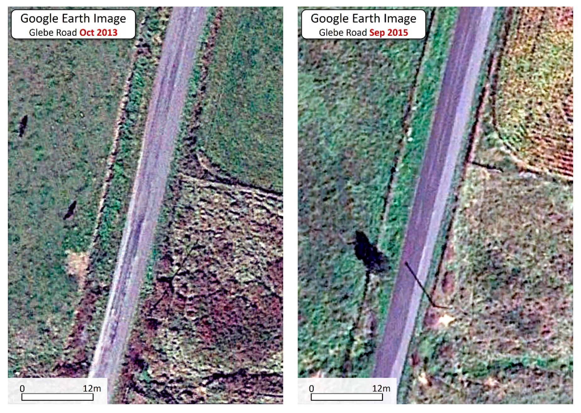
The pronounced presence of type-I errors (bad road segments misclassified as good road segments) along this stretch of road suggests that road maintenance may have occurred between the collection of the IRI and SAR data samples. Such road maintenance would have reduced road roughness and would explain the mismatch between SAR backscatter and IRI measurements. We contacted VDOT regarding potential maintenance activities around the acquisition time of the relevant SAR images and have indeed been informed that repaving was done along the identified road segment in the days before the acquisition of the X-band SAR data (phone calls to the regional field office revealed that the maintenance work was performed but not yet documented in the central office database). This repaving effort is visually evident in repeated optical remote sensing imagery available through Google Earth. The left panel of Figure 10 shows the condition of a short segment of Glebe School Road in October 2013, revealing significant road roughness in the form of rutting along the main road axis. In the September 2015 image (right panel of Figure 10), this rutting appears largely mitigated by the repaving of the western side of the road (darker road surface). The location of the road segment shown in Figure 10 is outlined by a black box in Figure 9b.

Based on the available information we can conclude that the observed difference between SAR-based IRI estimates and ground-truth data should not be considered a classification error. Instead, the classification results along Glebe School Road provide initial compelling evidence that the presented SAR-based amplitude mapping technique provides more up-to-date information about the current state of the road network and may be capable of identifying ongoing changes of pavement roughness conditions such as those related to often poorly documented road maintenance.

7.4. Potential Contribution of SAR Amplitude Data to Pavement Condition Mapping

7.4.1. Applicability to IRI Mapping by Road Category

As mentioned in the introduction, road roughness mapping is an important but also a labor- and cost-intensive responsibility of the US state DOTs. Based on the analyses in Section 7.1, Section 7.2 and Section 7.3, we conclude that X-band SAR is not well suited to assist in the road quality mapping of interstates and other roads of similarly high pavement quality. This is because 80% of all interstates in our area of interest have IRI values below $IRI=73 \mathrm{inches}/\mathrm{mile}$, which is the minimum IRI value that could be mapped with significance by X-band SAR from our study.

Instead, we found X-band SAR amplitude data to be a valuable tool for the network-level mapping of IRI values on secondary roads, with the goal of identifying and prioritizing pavement maintenance needs. In Augusta County, 95% of all IRI samples on secondary roads have IRI values larger than $IRI=73 \mathrm{inches}/\mathrm{mile}$ and can, therefore, be successfully analyzed and categorized using X-band SAR. As the IRI estimation accuracy is also typically higher for secondary roads, we conclude that X-band SAR can make valuable contributions to the quality assessment of this road type.

The potential contribution of SAR to IRI assessments on secondary roads can be significant due to the enormity of the IRI mapping task. For instance, only 20% of secondary roads can be scanned by the VDOT each year (random sampling, in addition to 100% of interstates and primary roads), requiring several years to prepare a complete assessment of the existing road network and causing significant gaps between repeated measurements. The inclusion of SAR data could, therefore, increase the timeliness of road information and lead to improved record keeping.

Through our serendipitous successful identification of recent repaving activities along Glebe School Road in Augusta County, VA, we could also hint at the capability of calibrated X-band SAR amplitude imagery to monitor changes of road roughness conditions on secondary roads, especially changes related to maintenance. Therefore, SAR may be useful in documenting road maintenance activities and in identifying sudden local changes of road quality as, for instance, caused by frost heave and greater than predicted pavement distress (post-construction performance monitoring). An in-depth analysis of the performance as well as an assessment of the limitations of SAR for this task is a subject of future work.

7.4.2. Cost Efficiency of SAR-Based IRI Mapping

The economic impact of SAR-based IRI mapping on a state DOT is difficult to assess. This is because such cost/benefit analyses need to consider a wide range of factors that are often not known or difficult to estimate. For the IRI mapping case, for instance, such factors include (i) the costs of traditional data collection via IRI field surveys, (ii) the expenses for maintenance activities that could be avoided if remote sensing enabled early intervention (foregone costs could require informed speculation at several levels), (iii) the costs of remote sensing data procurement, and (iv) the performance or effectiveness of the remote sensing approach used.

To make headway on a cost/benefit analysis, we collaborated with VDOT to develop a cost model that evaluates financial savings (if any) related to the inclusion of remote sensing approaches into VDOT’s road maintenance activities [28]. While this study focused on interferometric SAR (InSAR)-based early detection of sinkholes and unstable slopes, the methods and general conclusions derived in [28] are relevant for our IRI mapping scenario.

For the InSAR test case, the study found that VDOT cost savings sufficiently offset the costs of InSAR data analysis, justifying a technology “lease” period during which additional benefits from wide area monitoring could be explored. Additionally, under relatively conservative assumptions for detection rates (reflecting technology effectiveness) and savings rates (reflecting agency response), the analysis suggested that potential savings are sufficient over a 5-year analysis period with medium resolution (lower cost) InSAR data to provide funds for high resolution follow-up frames featuring “hot spots” or locations of special significance.

These findings together with the following considerations appear to be promising with respect to the potential economic impact of our IRI mapping concept on pavement evaluation activities:

• Currently, field surveys performed by VDOT are not comprehensive. As mentioned in Section 2, only about 20% of secondary roads are assessed by VDOT each year, resulting in several years delay before a specific road segment is resurveyed. Especially for secondary roads, this suggests that the addition of SAR could lead to improved early detection capabilities and associated reductions in road maintenance costs (see item (ii) in the above list).
• SAR data production costs for the presented IRI mapping application are expected to be significantly lower than those quoted in [28]. Due to the complexity of the required data analysis procedures, all InSAR processing tasks in [28] were outsourced to a specialty contractor, significantly increasing the SAR data production budget. As the IRI processing workflow is comparatively straightforward, the processing could be handled in-house (improvements to item (iii) in the above list).
• The InSAR processing method [SqueeSAR; 25] used in [28] necessitated the procurement of a densely sampled, multi-year stack of commercial high-resolution X-band SAR data. Therefore, data purchasing costs considered in [28] were substantial. As VDOT is performing IRI mapping only on an annual basis, data procurement costs would be comparatively low (improvements to item (iii) in the above list).

In summary, while the true economic benefit of adding SAR to the existing DOT tools is yet to be determined, the above considerations should provide a good justification for initiating further pilot studies aimed at quantifying the economic benefit of SAR-based IRI mapping methods.

7.4.3. Mitigating Sources of Error and Data Availability Limitations

We found trees nearby road centerlines to be a source of misclassification in our area of interest. We propose that existing land cover information should be used to identify and remove areas prone to misclassification by SAR before IRI mapping results are being submitted to a Department of Transportation. Regularly acquired high-resolution optical data such as the imagery provided by the Maxar Digital Globe or Planet spaceborne sensor constellations could also be integrated for this task.

Road obstructions may also be caused by man-made structures in the vicinity of roads such as those found in places where roads lead through population centers. As most of the US primary and secondary road system stretches through rural environments where urban settings are sparse and population densities are low, we expect that impacts of buildings on IRI mapping from SAR may be less prevalent than the impact of vegetation. Moreover, here, areas prone to obstructions can be flagged using appropriate reference information such as land use maps or optical imagery.

The presented approach is critically dependent on the availability of high-resolution X-band SAR imagery over an area of interest. Fortunately, the number of sensors providing such data has been continuously growing over the last few years. In addition to the established constellation of TerraSAR-X, TanDEM-X, and Cosmo-SkyMed sensors, access to the Korean KOMPSAT-5 has improved and new systems such as the Spanish PAZ X-band SAR were recently launched [29]. Interesting are also the upcoming X-band SAR constellations of the NewSpace companies Capella Space and ICEYE. Their spaceborne assets will provide meter-resolution SAR data at high temporal sampling (every few hours) and may provide further capabilities to US DOTs. However, whether or not the signal-to-noise and calibration performance of these sensors is sufficient for the task of pavement roughness assessment has yet to be determined.

8. Summary and Conclusions

Transportation infrastructure-related applications are a new and growing field in radar remote sensing. While most of the current remote sensing research is focused on detecting infrastructure deformation using InSAR techniques [30,31,32,33], this paper proposes the analysis of road surface quality using SAR amplitude information. We have analyzed X-band SAR data from the Cosmo-SkyMed constellation over an extended area in Virginia and found a significant correlation of X-band backscatter data with pavement roughness as measured by the IRI parameter. We developed a signal model to describe this correlation and estimated its parameters via a least-squares fit to the available data points. An inversion of the best-fitting nonlinear model performed well in classifying roads into “good roads” and “roads in need of repair” classes. For an area near Staunton, VA, an overall classification accuracy of 92.6% was achieved.

In addition to periodically assessing the current condition of road pavement, we also indicated the potential of SAR for providing timely information on local changes in road surface conditions such as those related to road maintenance. This was achieved by correctly identifying road segments that were repaved just before the acquisition of the X-band SAR image data.

An analysis of the accuracy of SAR-based IRI estimates revealed a strong dependence of estimation performance on IRI. We conclude that as estimation accuracy increases with IRI, SAR-based methods are currently most suitable for monitoring secondary roads. As currently used field data collection methods allow for only a relatively small percentage of secondary roads to be surveyed each year, the capabilities of satellite-based SAR to map secondary roads could lead to a significant improvement in the timeliness and frequency with which road quality information can be provided.

Future work will include more performance tests of the developed algorithms, specifically by applying it to other road networks in the US. Note that the signal function may have to be adjusted when applied to areas with very low road quality (IRI > 300). Other future work will include the application of the developed technique to time series of SAR data to further investigate the performance, as well as identify potential limitations of the SAR-based method to identify temporal changes of IRI.

References

- Gillespie, T.D. Measuring Road Roughness and Its Effects on User Cost and Comfort: A Symposium; ASTM International: West Conshohocken, PA, USA, 1985; Volume 884. [Google Scholar]
- Carey, W.N., Jr.; Irick, P.E. The Pavement Serviceability-Performance Concept; Highway Research Board: Washington, DC, USA, 1960; Volume 250, pp. 40–58. [Google Scholar]
- Sayers, M.W. On the Calculation of International Roughness Index from Longitudinal Road Profile; Transportation Research Board: Washington, DC, USA, 1995; pp. 1–12. [Google Scholar]
- Loizos, A.; Plati, C. Evolutional process of pavement roughness evaluation benefiting from sensor technology. Int. J. Smart Sens. Intell. Syst. 2008, 1, 370–387. [Google Scholar] [CrossRef]
- Emery, W.; Singh, M.C. Large-Area Road-Surface Quality and Land-Cover Classification Using Very-High Spatial Resolution Aerial and Satellite Data; RITARS-12-H-CUB; U.S. Department of Transportation: San Francisco, CA, USA, 2013.
- Emery, W.; Yerasi, A.; Longbotham, N.; Pacifici, F. Assessing paved road surface condition with high resolution satellite imagery. In Proceedings of the IEEE International Geoscience and Remote Sensing Symposium (IGARSS), Quebec, QC, Canada, 13–18 July 2014; pp. 1–4. [Google Scholar]
- Suanpaga, W.; Yoshikazu, K. Riding quality model for asphalt pavement monitoring using phase array type L-band synthetic aperture radar (PALSAR). Remote Sens. 2010, 2, 2531–2546. [Google Scholar] [CrossRef]
- Rosenqvist, A.; Shimada, M.; Ito, N.; Watanabe, M. ALOS PALSAR: A Pathfinder Mission for Global-Scale Monitoring of the Environment. IEEE Trans. Geosci. Remote Sens. 2007, 45, 3307–3316. [Google Scholar] [CrossRef]
- United States Census Bureau. U.S. Population Density (By Counties). Available online: https://www.census.gov/dmd/www/pdf/512popdn.pdf (accessed on 19 April 2020).
- VDOT. Virginia Department of Transportation Daily Traffic Volume Estimates Including Vehicle Classification Estimates—Jurisdiction Report 07; Virginia Department of Transportation (VDOT), 2015; p. 113. Available online: http://www.virginiadot.org/info/ct-trafficcounts.asp (accessed on 19 April 2020).
- United States Census Bureau. QuickFacts, Augusta County, Virginia. Available online: https://www.census.gov/quickfacts/augustacountyvirginia (accessed on 19 April 2020).
- Virginia Department of Transportation. Road Design Manual. Chapter 2E, Appendix A-1. Richmond. 2005. Available online: https://www.virginiadot.org/business/resources/LocDes/RDM/Appendix_a1.pdf (accessed on 15 April 2020).
- Caltagirone, F.; Capuzi, A.; Coletta, A.; De Luca, G.F.; Scorzafava, E.; Leonardi, R.; Rivola, S.; Fagioli, S.; Angino, G.; L’Abbate, M. The COSMO-SkyMed dual use Earth observation program: Development, qualification, and results of the commissioning of the overall constellation. IEEE J. Sel. Top. Appl. Earth Obs. Remote Sens. 2014, 7, 2754–2762. [Google Scholar] [CrossRef]
- Ulaby, F.; Long, D. Microwave Radar and Radiometric Remote Sensing; University of Michigan Press: Ann Arbor, MI, USA, 2015. [Google Scholar]
- Sayers, M.; Gillespie, T.D. The Ann Arbor Road Profilometer Meeting; U.S. Department of Transportation: Washington, DC, USA, 1986; p. 226.
- Calabrese, D.; Cricenti, A.; Grimani, V.; Scaranari, D.; Vigliotti, R.; Covello, F.; Marano, G. COSMO-SkyMed: Calibration & validation resources and activities. In Proceedings of the Radar Conference, Rome, Italy, 26–30 May 2008; pp. 1–6. [Google Scholar]
- Pettinato, S.; Santi, E.; Paloscia, S.; Pampaloni, P.; Fontanelli, G. The Intercomparison of X-Band SAR Images from COSMO-SkyMed and TerraSAR-X Satellites: Case Studies. Remote Sens. 2013, 5, 2928–2942. [Google Scholar] [CrossRef]
- Meyer, F.J.; McAlpin, D.B.; Gong, W.; Ajadi, O.; Arko, S.; Webley, P.W.; Dehn, J. Integrating SAR and derived products into operational volcano monitoring and decision support systems. ISPRS J. Photogramm. Remote Sens. 2015, 100, 106–117. [Google Scholar] [CrossRef]
- Ajadi, O.A.; Meyer, F.J.; Webley, P.W. Change Detection in Synthetic Aperture Radar Images Using a Multiscale-Driven Approach. Remote Sens. 2016, 8, 482. [Google Scholar] [CrossRef]
- Small, D. Flattening Gamma: Radiometric Terrain Correction for SAR Imagery. IEEE Trans. Geosci. Remote 2011, 49, 3081–3093. [Google Scholar] [CrossRef]
- Gesch, D.; Oimoen, M.; Greenlee, S.; Nelson, C.; Steuck, M.; Tyler, D. The national elevation dataset. Photogramm. Eng. Remote Sens. 2002, 68, 5–32. [Google Scholar]
- Johnsen, H.; Lauknes, L.; Guneriussen, T. Geocoding of fast-delivery ERS-l SAR image mode product using DEM data. Int. J. Remote Sens. 1995, 16, 1957–1968. [Google Scholar] [CrossRef]
- Small, D.; Zuberbühler, L.; Schubert, A.; Meier, E. Terrain-flattened gamma nought Radarsat-2 backscatter. Can. J. Remote Sens. 2012, 37, 493–499. [Google Scholar] [CrossRef]
- Small, D.; Miranda, N.; Ewen, T.; Jonas, T. Reliably Flattened Radar Backscatter For Wet Snow Mapping From Wide-Swath Sensors. In Proceedings of the ESA Living Planet Symposium, Edinburgh, Scottland, 9–13 September 2013; p. 91. [Google Scholar]
- Ferretti, A.; Fumagalli, A.; Novali, F.; Prati, C.; Rocca, F.; Rucci, A. A New Algorithm for Processing Interferometric Data-Stacks: SqueeSAR. IEEE Trans. Geosci. Remote Sens. 2011, 49, 3460–3470. [Google Scholar] [CrossRef]
- Su, X.; Deledalle, C.-A.; Tupin, F.; Sun, H. Two steps multi-temporal non-local means for SAR images. In Proceedings of the Geoscience and Remote Sensing Symposium (IGARSS), Munich, Germany, 22–27 July 2012. [Google Scholar]
- Sun, L. Simulation of pavement roughness and IRI based on power spectral density. Math. Comput. Simul. 2003, 61, 77–88. [Google Scholar] [CrossRef]
- Moruza, A.K. Economic Analysis of InSAR Technology Application in Transportation. In Proceedings of the Transportation Research Board 96th Annual Meeting, Washington, DC, USA, 8–12 January 2017. Paper No. 17-02179. [Google Scholar]
- Rodriguez, M.G.; Munoz, J.M.C.; Bonilla, M.J.G. PAZ First Results: Instrument Monitoring. In Proceedings of the EUSAR 2018; 12th European Conference on Synthetic Aperture Radar, Aachen, Germany, 4–7 June 2018. [Google Scholar]
- Vaccari, A.; Batabyal, T.; Tabassum, N.; Hoppe, E.J.; Bruckno, B.S.; Acton, S.T. Integrating Remote Sensing Data in Decision Support Systems for Transportation Asset Management. Transp. Res. Rec. 2018, 2672, 23–35. [Google Scholar] [CrossRef]
- Hoppe, E.; Bruckno, B.; Campbell, E.; Acton, S.; Vaccari, A.; Stuecheli, M.; Bohane, A.; Falorni, G.; Morgan, J.; Meyer, F.J. Transportation infrastructure monitoring using satellite remote sensing. In Proceedings of the Transport Research Arena (TRA) 5th Conference: Transport Solutions from Research to Deployment, Paris, France, 14–17 April 2014. [Google Scholar]
- Oliver, P.; Samson, C.; Kenny, S. Systematic preparation and processing of interferometric synthetic aperture radar data for monitoring linear transportation infrastructure. J. Appl. Remote Sens. 2019, 13, 024504. [Google Scholar] [CrossRef]
- Lazecky, M.; Hlavacova, I.; Bakon, M.; Sousa, J.J.; Perissin, D.; Patricio, G. Bridge displacements monitoring using space-borne X-band SAR interferometry. IEEE J. Sel. Top. Appl. Earth Obs. Remote Sens. 2016, 10, 205–210. [Google Scholar] [CrossRef]
© 2020 by the authors. Licensee MDPI, Basel, Switzerland. This article is an open access article distributed under the terms and conditions of the Creative Commons Attribution (CC BY) license (http://creativecommons.org/licenses/by/4.0/).