Article

A Textural Approach to Improving Snow Depth Estimates in the Weddell Sea

1
Department of Applied Ocean Science and Engineering, Woods Hole Oceanographic Institution, Woods Hole, MA 02540, USA
2
Department of Mechanical Engineering, Massachusetts Institute of Technology, Cambridge, MA 02139, USA
*
Author to whom correspondence should be addressed.
Remote Sens. 2020, 12(9), 1494; https://doi.org/10.3390/rs12091494
Submission received: 10 April 2020 / Revised: 30 April 2020 / Accepted: 4 May 2020 / Published: 8 May 2020
(This article belongs to the Section Environmental Remote Sensing)

Abstract

:
The snow depth on Antarctic sea ice is critical to estimating the sea ice thickness distribution from laser altimetry data, such as from Operation IceBridge or ICESat-2. Snow redistributed by wind collects around areas of deformed ice and forms a wide variety of features on sea ice; the morphology of these features may provide some indication of the mean snow depth. Here, we apply a textural segmentation algorithm to classify and group similar textures to infer the distribution of snow using snow surface freeboard measurements from Operation IceBridge campaigns over the Weddell Sea. We find that texturally-similar regions have similar snow/ice ratios, even when they have different absolute snow depth measurements. This allows for the extrapolation of nadir-looking snow radar data using two-dimensional surface altimetry scans, providing a two-dimensional estimate of the snow depth with ∼22% error. We show that at the floe scale (∼180 m), snow depth can be directly estimated from the snow surface with ∼20% error using deep learning techniques, and that the learned filters are comparable to standard textural analysis techniques. This error drops to ∼14% when averaged over 1.5 km scales. These results suggest that surface morphological information can improve remotely-sensed estimates of snow depth, and hence sea ice thickness, as compared to current methods. Such methods may be useful for reducing uncertainty in Antarctic sea ice thickness estimates from ICESat-2.

Graphical Abstract

1. Introduction

Estimating sea ice thickness from remotely-sensed data (here, snow freeboard, which is the amount of snow and ice above water) requires either simultaneous snow depth measurements or some assumption about the snow distribution on the sea ice. With a snow freeboard (F) and snow depth (D), and assuming hydrostatic equilibrium, the sea ice thickness (T) may be estimated for some snow, ice and seawater densities ( ρ s , ρ i , ρ w ) as:
T = ρ w ρ w ρ i F + ρ s ρ w ρ w ρ i D
When estimating sea ice thickness (SIT) from large-scale snow freeboard data from laser altimetry where no coincident observations of snow depth are available (such as from airborne campaigns including some Operation IceBridge flights where no snow radar data is available [1], or more broadly from satellites, e.g., ICESat [2] or ICESat-2 [3]), one must estimate snow depth independently. Common approaches include using an empirical fit to in-situ data [4] or assuming that there is negligible ice freeboard (i.e., all the ice has been depressed by snow cover, and so F = D in Equation (1)). This is reasonable on a large scale (averaged over many kilometers), over which the majority of the sea ice surface may consist of relatively thin, undeformed ice. However, Mei et al. [5] showed that this assumption is not valid at local scales (<100 m), especially near deformed areas, which have a variable proportion of ice within the snow freeboard. Moreover, linear methods to convert surface elevation to snow depth (or ice thickness) implicitly assume a constant snow/ice ratio and also constant snow and ice densities, which may be valid when averaged over large scales but not at local scales e.g., [4,6]. To address this, Steer et al. [7] used empirical fits for two different regimes (high and low ice freeboard), and found that there was considerable variability in the empirical fits for high ice freeboard regimes, in particular at local (sub-kilometer) scales, suggesting that high-freeboard snow surfaces may be morphologically complex. Steer et al. also noted that linear regressions are much better suited to large-scale mean snow depth predictions, and speculated that sophisticated models that could estimate the proportion of snow within the snow freeboard would improve snow depth estimates. Indeed, most studies of snow on sea ice use large length scales (typically 12.5 km or 25 km), in order to match the resolution of satellite-measured sea ice concentration datasets e.g., [8]. However, higher resolution SIT estimation are not possible without better knowledge of the snow distribution.
Neither the distribution of snow, nor its relationship with the distribution of ice freeboard, is well understood. Kwok and Maksym [9] and Mei et al. [5] found a weak correlation between snow depth and surface roughness (standard deviation of F), which may be the result of snow being blown and accumulating around deformed ice features. This may also be simply because both snow freeboard and roughness, as well as snow depth and snow freeboard, are themselves correlated, especially at large length scales e.g., [10,11]. Snow depth and snow freeboard measurements have been analyzed in both the Arctic and Antarctic. Farrell et al. [12] showed that the uncertainty in snow depth was the largest contributor to the uncertainty in SIT, and also noting that the snow depth over heavily ridged (Arctic) ice was sometimes not retrievable. Kwok and Maksym [9] found that snow depths sampled in situ may be biased due to excessively thin and thick ice not being logistically feasible to sample, while radar-based measurements cannot resolve snow depths below 8 cm. Zhou et al. [13] recently showed that different models for snow depth can give high variations for snow density and depth, and in some cases this can be higher than climatology. Similarly, Mallett et al. [14] showed that assuming a constant snow density, and hence a constant radar penetration speed, biases the snow depth estimate. It is well known that the snow depth distribution is complex and snow features observed in situ on sea ice suggest variations in snow depth [15,16,17]. Improving our understanding of small-scale snow depth distribution would therefore greatly improve SIT estimates.
Excluding drill line studies, which are logistically constrained to ice that is easily accessed by ship (not to mention easily drilled) e.g., [6,18], there are relatively few studies that look at the relationship between snow depth and SIT at the sub-kilometer scale, in particular in the Antarctic. For the Arctic, Petty et al. [19] used the Operation IceBridge (OIB) Airborne Topographic Mapper (ATM) altimetry data to show that the sea ice surface topography could be related to the sea ice thickness, by using a segmentation approach with high-resolution, three-dimensional lidar data. There have been, to date, no analogous work for the Antarctic, although Mei et al. [5] used high-resolution (terrestrial) lidar data to similarly demonstrate a link between the local surface topography and sea ice thickness.
For our study, we examine relationships between snow surface topography and snow depth by combining the OIB ATM and snow radar data, as they have comparable footprints/resolutions and are also measured concurrently. However, the snow radar data is from a nadir-looking radar and so is measured only along-track (i.e., it is a 1-D sequence of snow depths, unlike the lidar data, which is a 2-D collection of surface elevations). While we could simply use the intersection of these two datasets, this would essentially discard most of the lidar data, and limit ourselves to 1-dimensional studies by excluding any 2-D textural information in the lidar data. Moreover, there may be a sampling bias in the OIB data [9]. This motivates an extension of the snow radar data to the full lidar range. Mei et al. [5] showed that at local scales the ice freeboard cannot be assumed to be zero near deformed surfaces, so a more complex characterization of snow depth is needed. It may be possible to find relationships between surface morphology, or texture, and local snow depth distribution. If such textural relationships exist, this could then be used to provide an estimate of snow depth, and in turn an improved estimate of sea ice thickness from airborne or satellite altimetry.
Textural segmentation has been a long-studied problem in computer vision e.g, [20]. A variety of methods have been developed for this purpose, with differing advantages and disadvantages. As the evaluation of good textural segmentation results ultimately requires comparing to the subjective human eye, there is no single metric used to compare different methods, and as a result there is no single best method. Popular methods to achieve textural segmentation commonly include the use of either spatial or color-based metrics, or some combination thereof [21]. As our goal is to apply textural segmentation to lidar scans (analogous to grayscale imagery, as it has one input channel), we focus here on spatial metrics only.
The most common spatial metrics involve decomposing the image using some kind of convolutional filter. This essentially decomposes the image based on multiple frequencies of interest. Common examples include the Gabor transform [22], steerable pyramid decomposition [23,24], and the discrete wavelet transform [25]. In the context of sea ice, textural analysis has been largely limited to synthetic aperture radar (SAR) imagery for classification of the surfaces into some fixed number of classes. This includes the use of grey level co-occurrence matrices (GLCM) e.g., [26,27], wavelet transforms e.g., [28], and neural networks e.g., [29,30]. A detailed review of the state of sea ice classification using SAR data can be found in Zakhvatkina et al. [31]. There are few studies linking SIT to SAR images: Kim et al. [32] found a weak linear relationship between SIT and depolarization of return radar signatures may exist for deformed ice surfaces; Shi et al. [33] used a linear model with various SAR parameters to predict SIT; and Zhang et al. [34] found that the thickness of undeformed first-year ice < 0.8 m could be exponentially related to a ratio of the polarimetric scattering returns. Convolutional neural networks have been used to estimate sea ice concentration from SAR imagery [35]. However, SAR data is better suited for classification of sea ice types (e.g., with a convolutional neural network [35]) than for SIT estimation due to the ambiguity of the backscatter [36], and is not sensitive to snow depth.
Deep learning techniques can also be applied to predicting snow depths based of remotely-sensed data. Liu et al. [37] used an ensemble-based deep neural network using brightness temperature from passive microwave radiometry to predict snow depths with higher accuracy than linear regressions. Mei et al. [5] used a convolutional neural network to predict sea ice thickness, and showed that this method could be applied to predict local snow depth as well.
The aims of this paper are to show that snow distribution on sea ice may be characterized texturally using the snow freeboard spatial variability, allowing the estimation of snow depth when no direct measurement is available. Here, we show this by using textural information to extrapolate the spatially-limited snow depth data from the OIB snow radar. These area-averaged snow depths are then modelled using a convolutional neural network (ConvNet) that predicts the snow depth given an input lidar (snow freeboard) window. We compare the generalization of the ConvNet on a different dataset from a different year with a linear regression between F and D. We then examine our texturally-based snow depth estimates to the OIB measurements to estimate the sampling bias in the OIB snow depth dataset. We then use our snow depth estimates to estimate the uncertainty in predicting SIT using the OIB snow freeboard data.

2. Data and Preprocessing

The main source of data for this work are the Airborne Topographic Mapper (ATM) L1B elevation datasets and the Snow Radar L1B radar echo strength profiles, both available from the National Snow and Ice Data Center (www.nsidc.org). The snow depths are computed from the radar echograms following Kwok and Maksym [9]. We focus specifically on Weddell Sea flights from 28 October 2010 and 17 October 2016 (Figure 1).
The ATM surface elevation data consists of a conically-scanning laser altimeter with a footprint of ∼1 m, swath width of ∼250 m, vertical precision/accuracy of 3 cm/6.6 cm and shot spacing of a few meters [38]. Before the snow surface can be analyzed, the ellipsoid-referenced (World Geodetic System 1984) surface elevations must first be adjusted for the local sea surface height. This is done by using a reference geoid (EGM2008), which is accurate to a few meters, and then fine-tuned using nearby areas of open water (leads). This is further described in Section 2.1.
The OIB snow depth measurements are collected using a frequency-modulated continuous-wave snow radar [39]. This type of radar has been demonstrated in one field study to accurately retrieve snow depth [40]. The footprint is ∼7 m, with ∼1 m along-track resolution, though the effective resolution is 5.6 m due to decimation and boxcar-filtering of the signal [41]. More details can be found in Kwok and Maksym [9], Panzer et al. [39].

2.1. Snow Freeboard Data

The lidar ATM ellipsoid-referenced elevations are first converted into local lead-referenced snow surface freeboards. To do this, we first subtract the geoid (EGM-2008 at 1 minute resolution), and then we use local lead elevations as references. Identifying leads in the lidar altimetry is difficult, with various algorithms proposed. As presented in Kurtz [1], Onana et al. [42] used coincident camera imagery to look for leads directly, with extra filters to remove clouds and shadows. Kwok and Maksym [9] used the raw reflectivity data to isolate leads, which have lower reflectivity than ice. Wang et al. [43] found that in the absence of lead detections, using the lowest 0.2% percentile elevation values of the lidar freeboard gives a reasonable approximation to the lead elevation, when taking large (30 km) segments. These lead-referenced surface elevations, hence called ‘snow freeboard’ measurements, can then be combined with measured or assumed snow depths to estimate sea ice thickness.
Leads are identified using the Digital Mapping System onboard the OIB flights that takes synchronous digital imagery while the lidar/radar are operating [44]. The method is similar to the SILDAMS algorithm presented by Onana et al. [42]. We use just the grayscale imagery, and identify the peaks corresponding to open water, gray ice, and white ice, and then find the corresponding lidar points in each area (noting that some images may not have all three of these). An example is shown in Figure 2. We also exclude shadows and clouds from the lead detection, and manually verify the detected leads. A list of lead elevations and their longitude/latitude are compiled, and then the geoid-corrected ATM data is referenced to the local sea surface height. The local sea surface height is determined by an inverse-distance weighted elevation for all the leads within ±5 km. This distance is chosen in order to be within the first baroclinic Rossby radius of deformation (∼10 km at polar latitudes) for a given point, which is the typical length scale of eddies that create nonlinear perturbations on the sea surface height [45]. If there are not at least two leads identified within a ±5 km, the lidar point is discarded. The lidar is interpolated onto a grid with 1 m spacing using natural neighbor [46], and then windowed into 180 m × 180 m windows for later use in deep learning. Lidar points over water are masked and discarded from analysis, as there are relatively few returns which can introduce artifacts into the interpolation. These were excluded by identifying windows that had lead-referenced snow freeboards at the 3rd percentile of 0.0 m or lower. Lidar points with snow freeboard greater than 5 m are also excluded, as these are likely to be low-lying clouds or icebergs. Our lead accuracy is typically better than 3 cm, which is comparable to other studies like Kwok and Kacimi [8].

2.2. Snow Radar Data

Snow depths are retrieved from the OIB L1B Radar Echo Strength Profiles [47]. The radar returns are processed to find the signal peaks, and carefully checked to exclude the effects of sidelobes [48,49]. To account for the different travel speed of electromagnetic waves in snow, the return paths were scaled using the first-order approximation of the relationship between v c (the ratio of its speed compared to the speed of light in vacuum) and density ρ (g cm 3 ), v c = 1 2 ρ + 1 [50]. Taking a typical density of 300 kg m 3 following studies like Massom et al. [51], Arndt and Paul [52], this gives v c = 0.79 . For our two datasets, 34–36% of the radar returns were successfully processed into snow depths. This may introduce sampling bias; see Section 5.1 for more details. The average number of successful snow radar returns is 14 per 180 m, or equivalently an average spacing of 12.5 m between returns.

3. Methods

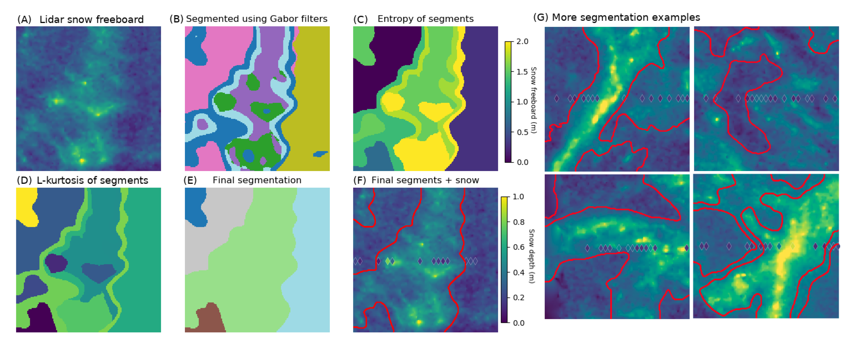
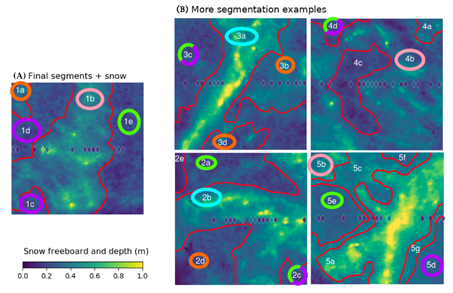
3.1. Textural Segmentation of Snow Surface

Our textural segmentation approach is based on the assumption that distinct sea ice types within a local region will have similar morphology, and will have experienced similar snow deposition conditions. For example, thicker ice of a similar age with similar ridge distribution that are nearby each other will likely have accumulated similar amounts of snowfall, and winds will have redistributed and shaped the snow cover on these floes in similar ways. Thinner young ice nearby would have a different growth and deformation regime, and accumulated a different snow depth distribution. A good example would be for a large floe that has subsequently broken into many smaller floes, with younger ice forming in the open water between the older floes. Similar assumptions were used in a simpler earlier study to extrapolate in-situ snow depths to a larger area Worby et al. [53].
Each lidar input (180 × 180 at 1 m resolution) is first normalized by the maximum snow freeboard in the window, to become an integer between 0–255. We use square windows so that these may also be used with deep learning methods described in Section 3.2. This essentially turns the lidar scans into grayscale imagery. From this, the local entropy is calculated, using a circular structuring element of size 10. However, it is still important to consider the characteristics of the snow freeboard values before normalization. For the lidar elevation measurements, the mean and standard deviation (computed on the non-normalized data, to preserve the effect of variations in freeboard among segments) have already been mentioned as relevant statistics: extending these to higher orders gives the skew and kurtosis. We use the linearized versions of these statistics, called the L-skew and L-kurtosis, which are more robust to outliers [54]. Outliers, in this scenario, would be extreme snow freeboard measurements, such as the sails of pressure ridges or extremely high snow depths. The skew is a measure of the asymmetry of the distribution, which is linked to how texturally uniform (or not) the snow surface is. The kurtosis is a measure of the ‘tailedness’ of a distribution, which may link to the proportion of deformation within a window.
We convolve a set of 20 Gabor filters with each window in order to distinguish different textural areas. The filters are oriented at 45, 90, 135 and 180 degrees, corresponding to wavelengths 2.8–45 m, with Gaussian kernels of size 11, standard deviation 7, zero phase offset and uniform spatial aspect. These hyperparameters were selected by manual experimentation. The filtered images are then passed through a nonlinear transducer (essentially a sigmoidal activation function using hyperbolic tangent) to accentuate high-activation areas, following Jain and Farrokhnia [55], and Gaussian-smoothed (kernel size 15). Filtered images with a low variance (below 0.0001) are discarded. The resulting feature vector consists of the filtered images and x and y coordinates of each pixel. Similar textures should have similar activations, and so the feature vector can be clustered using k-means clustering with a fixed number of clusters (here, we use 6, again manually chosen). We then look for contiguous segments (some of which may have the same cluster label) by using a standard open-source contour-finding method from Suzuki and Abe [56] implemented in OpenCV. Then, for each contour (segment), the neighboring segments are found, and their mean entropy and L-kurtosis are computed. These metrics were chosen by manually classifying 2000 images and using a decision tree to identify the most relevant metrics for distinguishing snow features from deformed ice. If the mean entropies of a segment and its neighbor are within 2.5%, and/or if the L-kurtosis are within 2%, then they are merged. Then, all segments are assigned a unique label. Small windows (less than 1% of the lidar window size) are erased and their pixels are ‘absorbed’ by their nearest neighbors. This is repeated until there are no more segments that can be merged. This process is summarized in Figure 3 and illustrated in Figure 4. We can now identify the segments that have snow depth measurements.
For each snow depth D within some segment, we work out the mean snow freeboard of the surrounding 7 m × 7 m lidar window (even if this window crosses into another segment), and take this mean value as F. We chose 7 m in order to match the snow depth footprint size. We then work out the F / D ratio. This essentially is a more complex version of Steer et al. [7], who used different empirical linear fits to different ice freeboard regimes. Then, all the ratios from each snow point are combined, and the maximum, minimum and average ratios are stored. The ‘average’ ratio here is defined as the harmonic mean, to prevent high F / D ratios (from ridges) from skewing the (arithmetic) mean high. The harmonic mean is generally preferred over the arithmetic mean when comparing ratios: this will be examined in Section 4.1.
To work out the extrapolated snow depth estimate for a given segment, we first compute the mean entropy, mean L-kurtosis, mean elevation and standard deviation for all segments. Then, for the target segment, we work out the average absolute difference in these four metrics for all other nearby (within a ±10 km range) segments. For this average, we use the geometric mean to account for the different scales of these metrics. All segments that are within a similarity threshold are identified. Their mean/max/min F / D ratios are compiled, and the average mean/max/min ratios are computed (as a weighted harmonic mean, weighted by similarity and also number of snow measurements in that segment. This ensures that segments with more snow measurements, and/or higher similarity, are weighted higher). The mean elevation of the target segment is divided by this (harmonically-)meaned ratio to determine the ‘true’ mean snow elevation of that segment. If there are at least 9 snow points amongst the identified nearby ‘similar’ segments, then the extrapolation is deemed a ‘successful completion’. An example for this is shown in the Appendix A.
In order to test the accuracy of this method, we first use only segments that contain snow radar measurements. For each segment, we compute the estimated mean snow depth using the extrapolation algorithm applied to that segment (and excluding that segment itself from the list of possible matches). We compare this estimate to the ‘true’ segment mean snow depth, which is computed as the segment mean F scaled by the harmonic mean of all F / D ratios taken at all snow depth measurement locations in that segment. We call this the ‘true’ mean snow depth, in contrast to the ‘raw’ mean snow depth which is just the (potentially biased) mean of all snow measurements in that segment. A variety of similarity thresholds were chosen; higher thresholds lead to more successful completions but higher errors. For all thresholds, using the weighted raw mean led to higher error than copying the F / D ratio instead. The proportion of successful completions is heavily affected by the chosen similarity threshold: higher thresholds allow more dissimilarity between ‘matched’ segments, which increases the completion rate. We chose a similarity threshold of 0.03, increasing in increments of 0.005 until 0.05, and keeping the threshold once at least nine snow points were being used for the extrapolation. This resulted in a 97% completion rate, a mean/median absolute error of 11.0 cm/6.6 cm, and a mean/median relative error of 39.1%/23.2%. It is important to note that these errors are an upper bound on the actual error, as the mean of the raw snow depths may not be an accurate estimate of the actual mean snow depth in that segment. This is particularly true for segments that have high snow depth variance but few radar observations, such as around large, deformed areas that have few snow depth measurements. If we only check the error for segments that have 9 or more snow depth measurements, which increases the likelihood that the sampled mean snow depth provides a reasonable estimate of the actual mean snow depth in that target segment, then the mean/median relative errors drop to 22.5%/16.4% and the mean/median absolute errors to 8.5 cm/5.6 cm.
Note that the harmonic mean F / D ratio is not the same as taking the ratio of the mean elevation and mean snow depth within a given floe segment. This is because the snow depths may be biased (in particular when the snow cover is too low to return), and also because the snow samples all fall on a fixed line, which may not be necessarily representative of the segment. In particular, we know that mean snow depths are biased high because the peak-finding algorithm does not return a snow depth when the snow is too thin (<7 cm). Taking the mean ratio attempts to address this bias, but still requires the assumption that the measured snow depths have a similar F / D distribution to the unmeasured snow depths. For comparison, we also apply the extrapolation algorithm to estimating the raw mean snow depth. The algorithm is the same, though instead of taking the weighted harmonic mean of the F / D ratios, we take a weighted arithmetic mean of the raw mean snow depths, again weighted by the number of samples per segment and the similarity. This gave slightly higher errors (mean/median: 25.5%/18.6%) than using the F / D ratio, again taking the error of segments with at least nine snow measurements only.

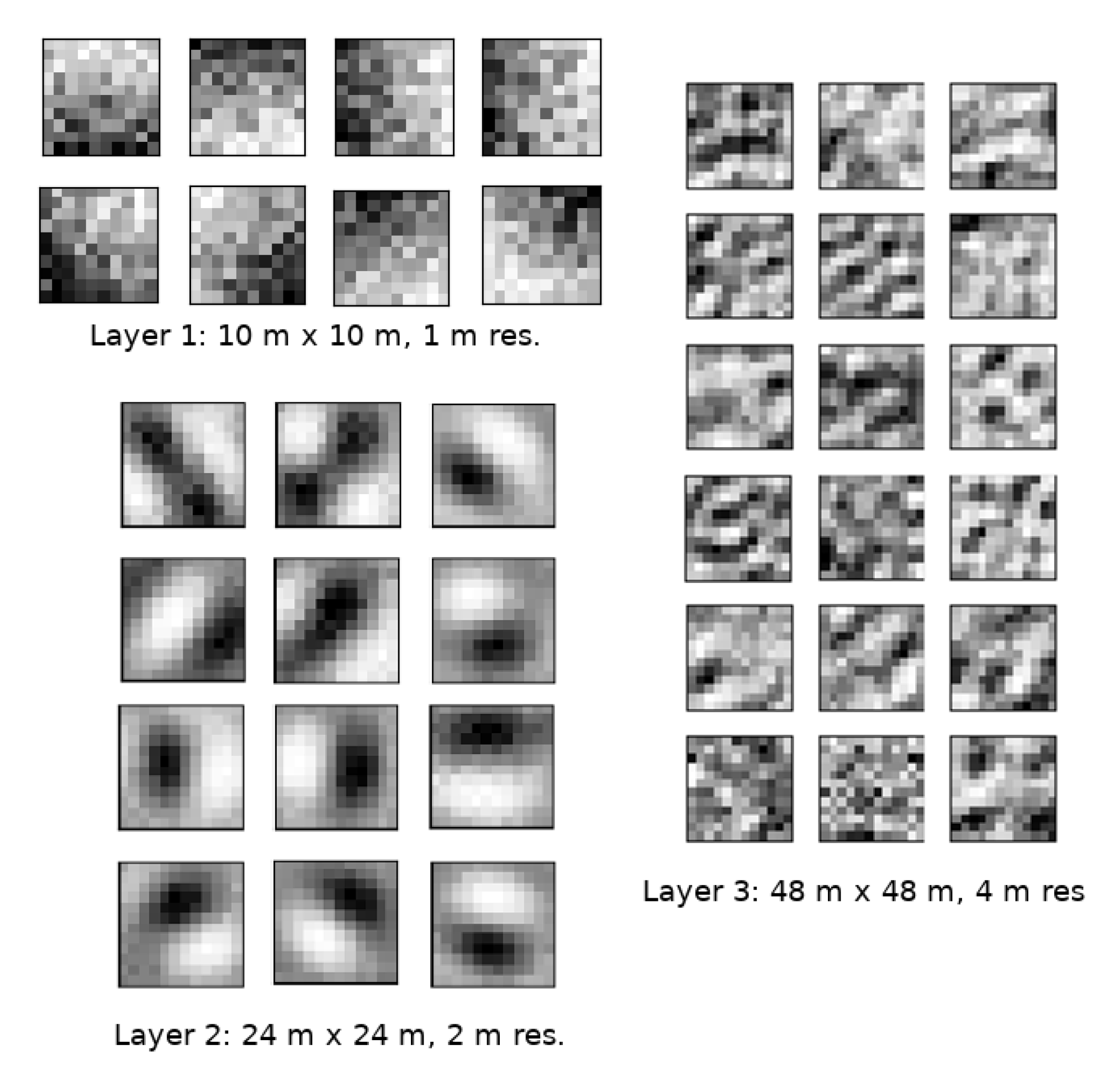
3.2. ConvNet for Learning Mean Snow Depth
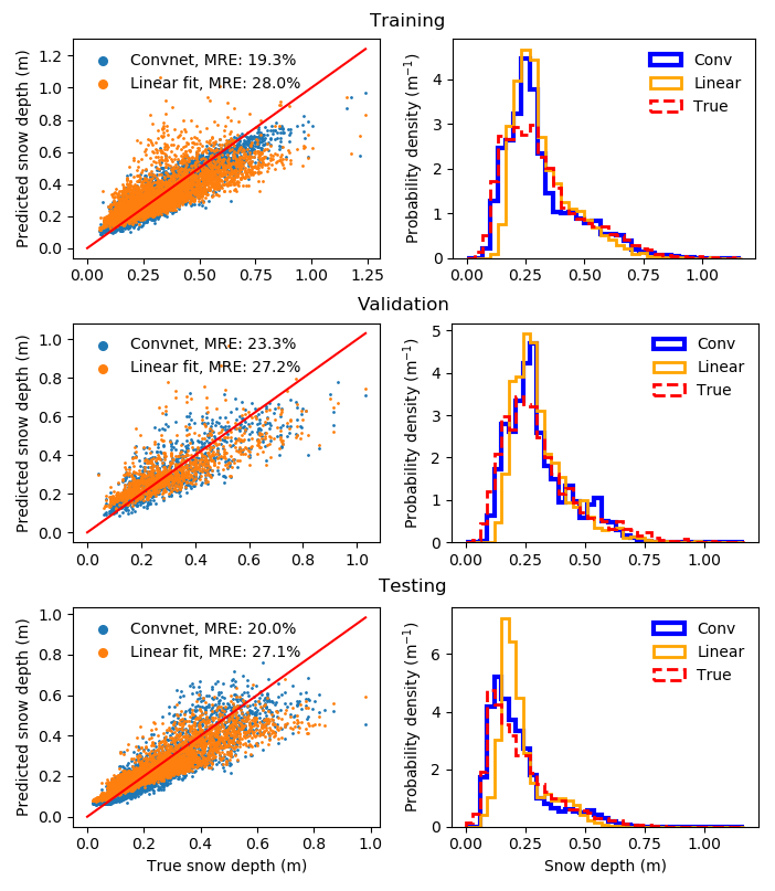
The previous sections presented a technique to estimate snow depths over a larger region given a small number of measurements based on snow surface texture. However, we now attempt to use deep learning to see if snow depth can be predicted directly from this snow surface texture only. To do this, we apply a convolutional neural network (ConvNet), as this is optimized to identify spatial features. This builds on our previous work which demonstrated this was effective in predicting snow and ice thickness at small scales [5]. Our ConvNet architecture is shown in Figure 5. As this is a regression problem, we used a mean squared error loss function. The inputs consist of 180 × 180 lidar windows. The true mean snow depths used for learning are the window-averaged ones as determined from the prior analysis. This provides a more robust mean snow depth estimate than the radar observations on their own when there are few snow depth observations, or when they may be biased by sampling only certain snow and ice regimes within the window. The learning rate was 8 × 10 4 , which gradually decreased to 7.2 × 10 5 . The optimizer used was Adam [57] with weight decay of 10 5 , and the activation function was SELU [58]. Each of four convolutional layers was implemented with a stride of 2, so that the data would be sub-sampled (in lieu of max-pooling). Two fully-connected layers were used in the final layers, to predict the mean snow depth of the input. 80% of the windows for the 2010 flight, randomly sampled, were used as the training set, and the remaining 20% were used as the validation set. The 2016 flight (the test set) provides a separate data set with different statistics that can be used to evaluate the efficacy of a ConvNet developed for one region or season against an independent dataset. As such, it can provide a measure of the ConvNet’s ability to generalize learned features to new datasets, which may allow it to detect variability in snow depth for other datasets, including those that lack snow depth observations.

4. Results

The relationship between D and F does not necessarily appear to be one-to-one. In Figure 6, we see the risk of using a mean snow value as a function of F: at high freeboards, the snow depth is likely to be either equal or nearly equal to snow freeboard or independent to snow freeboard, and using a mean value for local snow depth predictions will therefore always be wrong. For larger scale averaged snow measurements, an average measurement may be acceptable, but strictly speaking, this average should be weighted by the occurence of the two different regimes ( D = F and D is independent of F). This is naturally very influenced by sampling bias. The bimodality of the higher-F data also motivates the use of deep learning or other methods that can distinguish the different D values that may be associated with a high F.

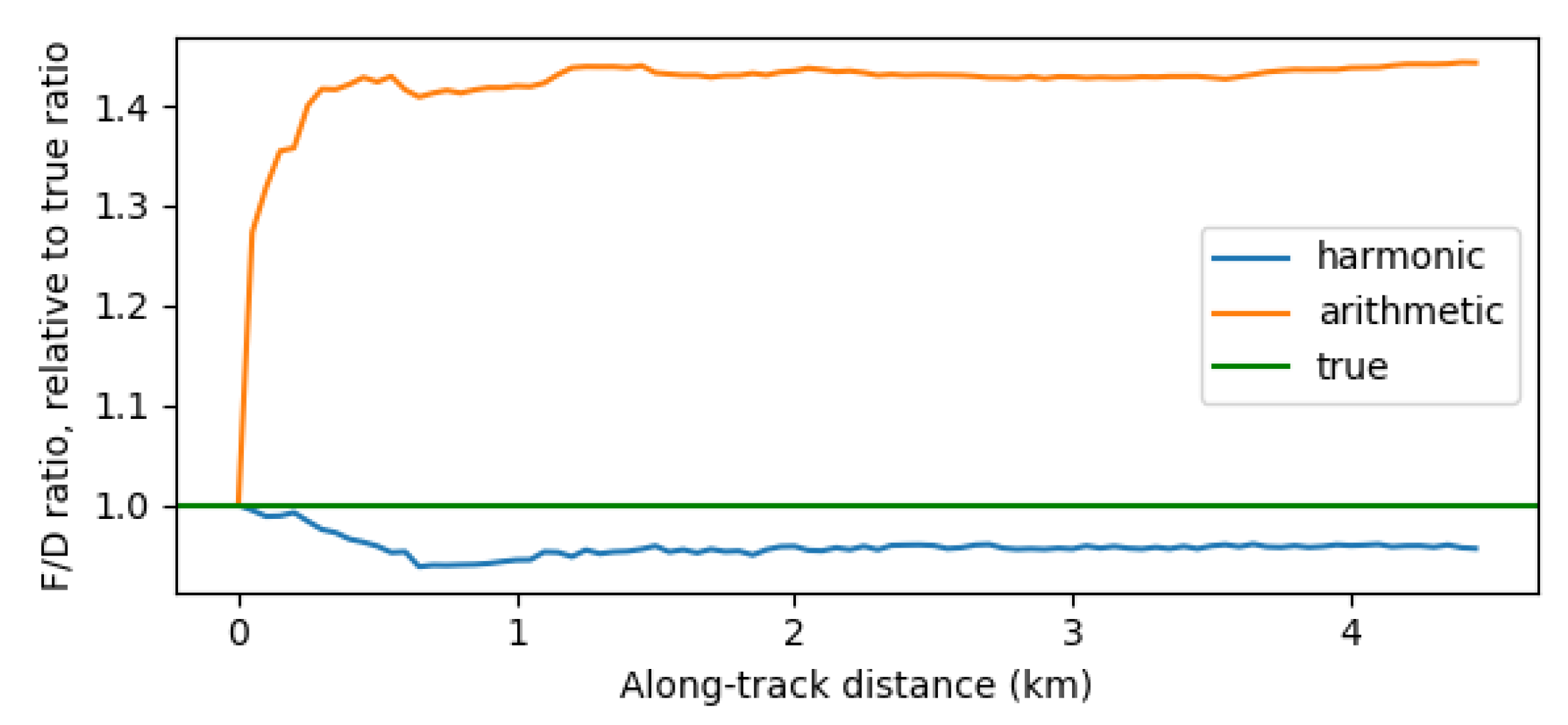
4.1. Extrapolated Snow Depths

The mean of all snow depth measurements for the 2010 dataset, assuming an average snow density of 300 kg m 3 , is 37.7 cm ( σ = 29.1 cm). The mean F corresponding to these points is 83.7 cm ( σ = 49.4 cm). However, the overall mean F for the entire set of lead-referenced snow freeboards (not just those with D measurements) is 72.6 cm ( σ = 53.6). This is suggestive of a sampling bias, as will be explored in Section 5.1. Assuming that the F / D ratio is the same for these two samples, this suggests that the true unbiased mean snow depth is closer to 32.7 cm. Using an empirical functional fit f ( F ) = D (for the mean snow depth for some given F as shown in Figure 6), f ( 72.6 cm) = 34.3 cm. The mean snow depth of the set of snow depth measurements that are contained within lidar windows is 38.2 cm. This is higher than the overall mean, likely because the lidar windows exclude any image with too much open water, where thin ice and thin snow are more likely to be found. If the (harmonic) mean F / D ratio for all corresponding snow points is applied to the mean F (76.0 cm) of the corresponding segments, the mean snow depth is 34.2 cm. This is slightly lower than taking the arithmetic mean of D (38.2 cm), in part because the snow depths do not sample thin snow (<7 cm) which likely have lower F. If applying the best empirical functional fit for snow depth (following the methodology of Kwok and Maksym [9]), the mean snow depth corresponding to F = 76.0 cm is 36.0 cm. Both the F / D ratio and empirical function suggest that the mean of the snow depth measurements is biased high, by 2–4 cm (around 10%). See Section 5.1 for further discussion of the biases in the snow data.
We find that both copying D and copying F / D lead to good accuracy in the overall survey-wide mean snow depth, within a few mm. Copying F / D has a lower mean relative error (MRE) of 22.5% than copying D directly (25.5%), and also a lower mean absolute error ( F / D : 8.5 cm; D: 9.4 cm). We therefore use F / D ratios for extrapolating the snow depths to those off-nadir segments that have no snow depths. As an additional advantage, using the F / D ratio accounts for the sampling bias for D just discussed. We have scaled the mean F / D ratio for each segment by 1/0.97, to correct for the tendency of the harmonic mean to slightly underestimate the true mean as shown in Figure 7. Note that our algorithm only looks for similar segments within 10 km, as we found that the error would increase along with a higher completion rate if we looked for similar segments in the full flight (mean error: 25.2%). We also tried looking for textural matches in the 2016 dataset to extrapolate the 2010 dataset, as a test of whether textural similarity generalized across datasets. This had slightly higher error (mean: 28.4%), suggesting the existence of common textural features for the same region/season but different years. Doing the reverse of this, i.e., extrapolating the 2016 dataset using the 2010 dataset, gave a similar, although slightly worse, mean error of 30.8%.

4.2. ConvNet Results

Results are summarized in Figure 8. The ConvNet had a lower training, validation and testing error than a corresponding linear regression fit to the F and D data. This is likely due to the ConvNet learning more advanced metrics and implicitly learning different F / D ratios, whereas a linear regression assumes one overall mean F / D ratio. More analysis regarding the ConvNet performance is given in Section 5.
Figure 9 shows the ConvNet and linear model results, as well as the raw (measured), window-averaged and extrapolated snow depths. When there are many raw points of a similar snow depth (e.g., near x = 2.5 km), the surface is likely fairly uniform and the radar-sampled snow depths are likely an unbiased sample of the true snow depth of the lidar window. The extrapolated snow depth (red) and raw mean (green) therefore are in good agreement. In contrast, near ridges, the measured snow depths have a greater vertical variability (e.g., the peak near x = 1.1 km has a snow depth of 0.9 m). For this example, the raw mean snow depth (green) exceeding the raw mean snow freeboard (black) is suggestive of a sampling bias, and in any case indicates that the mean of the raw snow depth measurements should not be taken as the true mean snow depth of the window. The snow depth samples are likely biased by the deep snow around the ridge, which may only be a minority of the surface, and so the raw mean snow depth (green) is higher than the extrapolated snow depth (red). Possible biases are discussed in greater detail in Section 5.1. Another point to note is that the linear model for snow depth necessarily assumes that similar (mean) freeboards have similar (mean) snow depths. In Figure 9, because the mean freeboards vary narrowly between 0.26–0.48 m, the linear estimate of the windowed snow depth also has a narrow range, of 0.15–0.24 m. In contrast, the raw and extrapolated snow means both have a higher range, of 0.11–0.34 m and 0.08–0.28 m respectively, which is matched by the ConvNet estimate of 0.08–0.27 m. The linear estimate has on average higher errors for predicting the snow depth at each window along this flight track (32% vs. 23% for the ConvNet). Similarly, the linear estimate has worse performance when estimating the extrapolated mean snow depth (15.5 cm) along the entire 5 km flight track (linear: 18.9 m, 22% error; ConvNet: 17.3 cm, 12% error).

5. Discussion

5.1. Effectiveness of Segment Texture-Matching

Snow depths corresponding to successfully matched segments are typically lower than the overall average. This is shown in Figure 10, which shows the distribution of the snow depth and freeboard for completed and non-completed segments. However, of the segments that are completed, the estimated mean from textural matching is very close, within 0.01 cm of the true mean. This is not the case if using the empirical function from Figure 6, which predicts a mean snow depth of 36.0 cm, which is 2.4 cm higher than the true mean. This is likely because, as shown in Figure 6, the relationship between F and D is not bijective, and at higher F values, the value for D may be bimodal: high snow freeboards may be thick snow dunes or deformed ice with little snow. If these regimes are texturally distinguishable, then the textural matching would lead to the right regime being picked, as opposed to always applying the average snow depth. One could use a weighted average of the two regimes in Figure 6 to work out the true survey mean snow depth, but this is highly subject to sampling bias (as thin snow has fewer returns). High-F segments are less likely to be texturally matched than low-F segments, perhaps because there are fewer such samples in general, and perhaps also because extremely rough ice reduces the number of successful snow radar returns e.g., [48]. This may lead to our estimated mean snow depth being biased slightly lower. However, as shown in Figure 10, our extrapolated snow distribution compares very well to the true snow distribution, and the estimate of the mean snow depth is only 0.01 cm lower. We can therefore be confident that the extrapolation algorithm, in and of itself, does not induce a significant bias.
There is another bias, one that results from the sampling of the snow depths due to thin snow being excluded. Our algorithm attempts to address this sampling bias, but it is not known if using the F / D ratio instead accounts for the entire sampling bias correctly. This is also shown in Figure 10 (green and blue lines). By comparing the distributions of the completions that do and do not have snow depths, we can see if segments that have an observed snow depth have different statistical properties to those that do not (which includes both segments that, if the radar flew over them, would have a snow depth and those that would not). This is effectively comparing whether the snow depth distribution where the radar was able to resolve the snow depth is different from the snow depth distribution in locations where it cannot. Their mean snow depth estimates are 33.6 and 29.0 cm respectively, suggesting a sampling bias of ∼+5 cm. This is in line with our finding from Section 4.1, which found that the mean snow depth was biased low by 2–4 cm because the mean F was slightly larger for snow depth sampling points than for the rest of the lidar scan and noting that larger F tends to be associated with larger D.
For the completions (27,921 segments), 50% (13,971 segments) have a snow depth, but for the non-completions (2049 segments), 35% (720 segments) had snow depths. As seen in Figure 10, the non-completions have a much higher mean F than the completions. This is in line with the non-completions having a higher average F (and D), as the rougher surfaces are fewer in number (i.e., harder to match), have greater variability (i.e., also harder to match), and are less likely to have a snow depth return [12]. This is consistent with our earlier finding that the extrapolated snow depths may be slightly biased low. Thus, there are two potential biases in the snow radar data: it is less likely to sample very deep snow in rough deformed ice, but also less likely to sample very thin snow. These biases will partially offset each other so the overall sample bias is low. However, the proportion of high snow freeboard is relatively low compared to the proportion of thin snow for this dataset, and so the net result is the raw mean snow depth is biased high, as we find. The bias from OIB may still be considerably less than in situ sampling. Our deepest snow depths are deeper than typically measured in situ on selected floes e.g., [51,52], in line with findings from Kwok and Kacimi [8].
The segment-matching algorithm has a trade-off between completion rate and accuracy. Higher completion rates imply extrapolating with lower-quality matches, which increase the uncertainty in the extrapolation. We noticed that ‘local’ matches (i.e., closer segments) give lower error estimates, but at the cost of a lower completion rate. The median relative error of using a ±5 km search grid for the textural matches is 23.6%; for ±10 km is 23.7%; using the full flight is 26.9%. This is consistent with our assumption that nearby ice floes with similar morphology will have experiences similar snow deposition regimes. However, using a different flight entirely (e.g., extrapolating the 2010 dataset using the 2016 dataset) gave a MRE of 28.2 % and a completion rate of 99.8%. This implies that textural features show some similarity across different years in the same region, although there is enough variation that the errors from using data from different years are slightly higher. This may mean that relationships between surface texture and snow depth exhibit universal or regional behavior. As such, this technique might be effective broadly around the Antarctic, although this needs to be confirmed with data from different regions that experienced different snow and ice regimes, such as the Bellingshausen and Amundsen Seas.
Our average F / D ratio of 2.0–2.2 is much higher than (although technically within error of) an equivalent Weddell Sea dataset from Polarstern 1988 (presented in Ozsoy-Cicek et al. [6]), which had F / D = 1.12 ( ± 0.9 ) . However, their data is from an in-situ drill line, which naturally is biased towards thinner ice (lower F) for typical ice conditions during this season (spring). This further suggests that drill line data may not be fully representative of the range of sea ice conditions needed to derive satellite ice thickness estimation algorithms. However, we note that there are no co-located in-situ snow depths on Antarctic sea ice to validate the OIB radar data, and it is possible that the radar underestimates true snow depth, although limited comparison does not suggest this is likely [9].

5.2. ConvNet Analysis

It is clear that the ConvNet performs well and is able to predict, with good generalization on the test set, mean snow depths. The mean test error of 20% is unlikely to be able to be reduced further, as the input data (extrapolated snow depths) themselves had a mean error of 22.5% (per segment-this is likely to be reduced when averaging over multiple lidar windows). We noticed that the reverse scenario (training on 2016 data and testing on 2010 data) gave comparable, although slightly worse results (test MRE: 27%). This is in line with our finding from Section 4.1 that the snow extrapolation was slightly worse for using the 2010 dataset to extrapolate the 2016 dataset than vice versa. It is possible that the features contained within the 2010 dataset are a superset of those contained within the 2016 dataset, and hence the snow extrapolation/ConvNet using the 2016 dataset as a basis is unable to fully capture the variability of the 2010 dataset.
To give us an idea of what the trained ConvNet is basing its prediction on, we look at examples of the learned filters for the first three convolutional layers (Figure 11). The first two layers appear to correspond to common filters in computer vision for edge detection and textural analysis e.g., [60], which would detect linear types such as ridges or boundaries between morphological regimes. The filters in the third layer are likely to be textural components (patterns), possibly snow dunes on level ice, or rubble fields.
One strength of the ConvNet over linear fits is its ability to predict the snow depth accurately at lower length scales. Figure 12 shows the error distributions when taking mean snow depths over segments of 1.5, 5, 10 and 25 km scales. In all cases, the total length of segments spanned by the segments exceeded 1000 km. As the length scale increases, the linear fit approaches the ConvNet, and both errors decrease. This is expected as the linear fit to the training data includes the many different surface types, and at such large length scales the variability in snow depths given some snow freeboard is low enough that linear fits are comparable. But at the smaller scales, the ConvNet performs much better, with fewer large errors. This is encouraging for the possibility of using a similar technique to improve snow depth and sea ice thickness estimation at smaller scales from ICESat-2.

5.3. Implications for SIT Estimates

Ultimately, an improved estimate of snow depth will permit an improved estimate of SIT. Here, we evaluate whether our technique to estimate snow depth might be sufficient to accurately estimate Antarctic SIT without an independent estimate of snow depth. The first-order uncertainty in estimating sea ice thickness ( ϵ T ) given laser altimetry (snow freeboard, F) and snow depth measurements (D), following Giles et al. [61], is given by:
ϵ T 2 = ϵ F 2 ( ρ w ρ w ρ i ) 2 + ϵ D 2 ( ρ s ρ w ρ w ρ i ) 2 + ϵ ρ s 2 ( D ρ w ρ i ) 2 + + ϵ ρ w 2 ( F D ρ w ρ i F ρ w + D ( ρ s ρ w ) ( ρ w ρ i ) 2 ) 2 + ϵ ρ i 2 ( F ρ w ( ρ w ρ i ) 2 + D ( ρ s ρ w ) ( ρ w ρ i ) 2 ) 2
Using the mean F and D values from our 1.5 km segments of 0.44 m and 0.22 m respectively, typical densities of ρ w = 1024 kg m 3 , ρ i = 915 kg m 3 , ρ s =300 kg m 3 , this gives:
ϵ T 2 = 88.3 ϵ F 2 + 44.1 ϵ D 2 + 4.07 × 10 6 ϵ ρ s 2 + 2.62 × 10 3 ϵ ρ w 2 + 6.01 × 10 4 ϵ ρ i 2
Our mean relative error of 14.0% for snow depth of the 1.5 km segments gives ϵ D = 0.033 m. We take a typical estimate of the seawater density variability of ±1 kg m 3 . We take ϵ ρ s = 50 kg m 3 , following Kwok and Maksym [9], which was based on variability in large-scale average snow depths observed in different regions and years [15]. The uncertainty from snow freeboard is likely due to the lead height accuracy, as well as the range resolution of the lidar. Over a 1.5 km segment, there are sufficient points that the range resolution of the lidar itself contributes little uncertainty. However, the lead height uncertainty (typically 3 cm, [9]) also contributes to the uncertainty. If there are two leads, each with RMS error 3 cm, then assuming the errors are distributed normally, the uncertainty of their average is 3 2 = 2.1 cm. As the local sea surface height is a weighted average of the nearby leads (in our case, inverse-distance weighting), the resulting variance is a weighted sum of each variance (for simplicity, we assume all leads have RMS error 3 cm), with the weights summed in quadrature. Working this out for all our lidar windows gives a weighted average variance of 0.54 σ 2 , which gives a snow freeboard uncertainty of ϵ F = 0.54 × 3.0 = 1.6 cm. The density of sea ice is a large source of uncertainty, due to the variable porosity of sea ice (and that the pores may be filled with either seawater, as is typical for first-year ice, or air, as is typical for multi-year ice), and variable (and unknown) macroporosity (space between rubble blocks) of ridges. We take the uncertainty in sea ice density as ϵ ρ i = 20 kg m 3 for first year ice following Maksym and Markus [62] (note, this would be considerably higher if we consider that the ice may be multiyear, summer sea ice, or ridges may be unconsolidated).
Putting these values into Equation (3), we have:
ϵ T 2 = 88.3 × 0.016 2 + 44.1 × 0.033 2 + 4.07 × 10 6 × 50 2 + 2.62 × 10 3 × 1 2 + 6.01 × 10 4 × 20 2 = 0.023 + 0.048 + 0.010 + 0.003 + 0.240 ϵ T = 0.57 m
From Equation (1), T = 2.79 ± 0.57 m and so our relative uncertainty in estimating SIT is 20%. This uncertainty is dominated by the term corresponding to ϵ ρ i . Excluding this, the contributions from ϵ ρ s , ϵ F and ϵ D are similar, and the contribution from ϵ ρ w is negligible.
Our average values for F and T compare well to Yi et al. [63], which looked at the Weddell Sea from October-December (their range for F: 0.33–0.41, T: 2.10–2.59). Our values are slightly higher than theirs, possibly because the OIB flights take place in October, when the F and T values may be slightly higher than in December (summer).

6. Conclusions

We have demonstrated the viability of extrapolating snow depth measurements from nadir-looking (1-dimensional) radar datasets from Operation IceBridge, by texturally segmenting the high-resolution lidar scan of the snow freeboard and then matching texturally-similar areas. We find that the ratio of the snow freeboard F and snow depth D, applied to the segment mean F, is a better predictor of the true segment mean snow depth than just copying in D values from these texturally-similar segments. This is likely because the freeboard provides a physical constraint on the snow depth. But it may also be indicative of a sampling bias present in the radar snow depths. We find evidence of a sampling bias in the snow depth data from OIB, which gives an overall bias of around +2–4 cm for the mean snow depth. This is likely because thin snow depths are not resolved by the snow radar, consistent with findings from Kwok and Maksym [9]. Our extrapolations for the snow depth have ∼22% error at 180 m scale by extrapolating from nearby floes. However, this error is only slightly larger (∼28%) if extrapolating from a completely different dataset. This suggests that there may be regional, or perhaps even generalizable relationships between surface texture and snow depth, although this needs to be evaluated for datasets from different regions and seasons.
Using this data, we show that the snow depth at 180 m scale can be predicted directly from the snow freeboard data using a convolutional neural network (ConvNet). The learned filters appear to correspond to standard textural analysis techniques, which suggests that there is a relationship between snow surface texture and snow depth. The error when applied to a different dataset from a different year is 20%, suggesting that there is, at least for the Weddell Sea, a connection between the texture of the snow surface and the snow depth. The 20% error (at 180 m scale) for our ConvNet may be irreducible as the snow depth data that it is being trained on itself has a similar error (∼22%). Predicting mean snow depths over a larger length scale (1.5 km) gives lower errors for the snow depth estimates (14%), which allows for a lower uncertainty in sea ice thickness estimates at the 1.5 km scale of ∼20%.
We find that the highest contribution to the sea ice thickness uncertainty, using our snow depth estimates from the ConvNet, is from the uncertainty in sea ice density. This suggests that estimating snow depth from sea ice surface texture alone may be sufficiently accurate to constrain SIT, and that improved treatment of sea ice density is now at least as important. However, this result needs further evaluation for other regions, such as the Bellingshausen/Amundsen sea, for which OIB snow depths are significantly deeper.
Ultimately, this work may provide insight into suitable length scales for snow depth analysis and suggestions of relevant metrics to predict snow depth for other high-resolution datasets, including, if the technique can be extended to linear topography data, ICESat-2.

Author Contributions

Conceptualization, M.J.M. and T.M.; Data curation, M.J.M.; Formal analysis, M.J.M.; Funding acquisition, T.M.; Methodology, M.J.M. and T.M.; Software, M.J.M.; Supervision, T.M.; Visualization, M.J.M.; Writing—original draft, M.J.M.; Writing—review & editing, T.M. All authors have read and agreed to the published version of the manuscript.

Funding

This research was funded by National Aeronautics and Space Administration grant number NNX15AC69G and the US National Science Foundation grant number ANT-1341513.

Acknowledgments

The authors would like to thank Ron Kwok for providing the snow depth data used in this study.

Conflicts of Interest

The authors declare no conflict of interest. The funders had no role in the design of the study; in the collection, analyses, or interpretation of data; in the writing of the manuscript, or in the decision to publish the results.

Appendix A. Example of Segment Matching

Figure A1 shows an example of the segment-matching algorithm in action. For this example, we only use a subset of nearby windows for clarity. All relevant metrics are for all segments shown are in Table A1. For example, for segment 1e, the only other segments it is matched to (here, we use a similarity threshold of 0.04 so that we can just have 2 segment matches) that contain snow depth measurements are 3c and 5e. The set of metrics M = { F , σ , entropy, L-kurtosis} for 1e is { 0.4349 , 0.096 , 3.841 , 0.152 } . Taking the differences between these values, M 1 e and their corresponding values for segments 3c ( M 3 c ) and 5e ( M 5 e ) gives | M 3 c M 1 e | = { 0.007 , 0.006 , 0.071 , 0.009 } and | M 5 e M 1 e | = { 0.173 , 0.003 , 0.022 , 0.073 } . Adding 0.001 to each value (to prevent taking a geometric mean with a zero) and then taking their geometric means to give the similarity metric S gives S 3 c = 0.0142 and S 5 e = 0.0330 . The number of snow depth measurements for each segment are N 3 c = 3 and N 5 e = 5 . The resulting estimate for the mean F / D ratio for 1e is the weighted harmonic mean of the ratios for segments 3c and 5e, weighted by N/S (normalized). We assume more points = more confidence in the textural match, and lower S = higher similarity = more confidence in the textural match. The (unnormalized) weights are therefore N 3 c / S 3 c = 3 / 0.142 = 212 and N 5 e / S 5 e = 5 / 0.0330 = 151 . To normalize, we simply divide the weights by their sum, to give a final weight of 0.58 for segment 3c and 0.42 for segment 5e. The mean ratio is determined by taking the weighted harmonic mean of the F/D ratios corresponding to segments 3c and 5e, i.e., 1 0.58 4.571 + 0.42 5.126 = 4.79 . The estimated snow for this segment is therefore F 1 e / 4.79 = 0.091 m. The true (extrapolated) segment mean snow depth (scaling F 1 e by the F / D ratio for that segment) should be 0.434 / 2.290 = 0.190 m, so the overall prediction error for this segment is 52% (or 9.9 cm). Note that in the full algorithm, instead of taking 4 nearby lidar windows, all lidar windows within ±10 km are checked for textural matches (potentially up to 120 windows). The similarity threshold is also higher in the real algorithm (0.050), which will also give more matching segments (in this example, it would also match 1e with 1d and 4c). Lastly, we require at least 9 snow depth samples to be used in the calculation, and so this particular example (that uses a total of 8 snow depth points) would be discarded as a low-quality estimate.
Figure A1. Example segment matching, for a similarity threshold of 0.04. Segments are color-coded to show their textural matches: 1a is matched to 2b, 3b, 3d; 1b is matched to 4b, 5b; 1c is matched to 1d, 2c, 3c, 4d, 5d; 1e is matched to 2a, 2c, 3c, 4d, 5e and 2b is matched to 3a.
Remotesensing 12 01494 g0a1
Table A1. List of metrics for the segments in Figure A1: the segment ID, the segment area, the number of snow depth samples in that segment (N), the mean of all raw snow depth measurements (D), the mean snow freeboard for the whole segment (F), the standard deviation of the snow freeboard ( σ ), the mean entropy of the segment, the L-kurtosis of the segment snow freeboard. F / D is the harmonic mean of all snow depth measurements within the segment and the corresponding mean snow freeboard for that snow radar footprint. This means that F / D is not the same as taking the quotient of the F and D columns.
IDArea (m 2 )ND (m)F (m) σ (m)EntropyL-Kurtosis F / D
1a11430-0.62550.1334.3570.191-
1b16,45480.25460.8050.2094.5060.1333.72
1c10900-0.48330.0744.0160.092-
1d503220.15000.4910.0743.7320.1213.34
1e868130.20330.4340.0963.8410.1522.29
2a63740-0.42770.1134.1500.111-
2b18,009130.23550.8870.2744.7260.0973.83
2c10010-0.42790.1034.0880.119-
2d62760-0.41600.1383.9810.193-
2e7400-0.23130.0713.7990.027-
3a16,02750.25550.8640.4094.7530.0843.00
3b769870.15730.6600.1544.2090.2004.31
3c645130.10390.4410.0903.7700.1434.57
3d22240-0.48310.1484.4000.187-
4a9640-0.68830.1054.1170.147-
4b25,523160.16800.6370.1974.4720.1373.44
4c478410.13220.3740.0864.0240.1282.75
4d11290-0.40860.0783.9370.118-
5a14,75260.33051.3130.2914.9440.1234.43
5b15210-0.95370.2034.6780.139-
5c725110.13050.7790.1604.4310.2465.27
5d242410.21690.6360.0763.6080.0973.16
5e448650.12810.6070.0933.8190.0795.12
5f5480-0.67330.0793.9350.056-
5g141820.34060.8400.0834.2650.1882.26

References

  1. Kurtz, N. IceBridge quick look sea ice freeboard, snow depth, and thickness product manual for 2013. NSIDC 2013. [Google Scholar] [CrossRef]
  2. Zwally, H.J.; Yi, D.; Kwok, R.; Zhao, Y. ICESat measurements of sea ice freeboard and estimates of sea ice thickness in the Weddell Sea. J. Geophys. Res. Ocean. 2008, 113. [Google Scholar] [CrossRef] [Green Version]
  3. Markus, T.; Neumann, T.; Martino, A.; Abdalati, W.; Brunt, K.; Csatho, B.; Farrell, S.; Fricker, H.; Gardner, A.; Harding, D.; et al. The Ice, Cloud, and land Elevation Satellite-2 (ICESat-2): Science requirements, concept, and implementation. Remote Sens. Environ. 2017, 190, 260–273. [Google Scholar] [CrossRef]
  4. Xie, H.; Tekeli, A.E.; Ackley, S.F.; Yi, D.; Zwally, H.J. Sea ice thickness estimations from ICESat Altimetry over the Bellingshausen and Amundsen Seas, 2003–2009. J. Geophys. Res. Ocean. 2013, 118, 2438–2453. [Google Scholar] [CrossRef]
  5. Mei, M.J.; Maksym, T.; Weissling, B.; Singh, H. Estimating early-winter Antarctic sea ice thickness from deformed ice morphology. Cryosphere 2019, 13, 2915–2934. [Google Scholar] [CrossRef] [Green Version]
  6. Ozsoy-Cicek, B.; Kern, S.; Ackley, S.F.; Xie, H.; Tekeli, A.E. Intercomparisons of Antarctic sea ice types from visual ship, RADARSAT-1 SAR, Envisat ASAR, QuikSCAT, and AMSR-E satellite observations in the Bellingshausen Sea. Deep Sea Res. Part II Top. Stud. Oceanogr. 2011, 58, 1092–1111. [Google Scholar] [CrossRef]
  7. Steer, A.; Heil, P.; Watson, C.; Massom, R.A.; Lieser, J.L.; Ozsoy-Cicek, B. Estimating small-scale snow depth and ice thickness from total freeboard for East Antarctic sea ice. Deep Sea Res. Part II Top. Stud. Oceanogr. 2016, 131, 41–52. [Google Scholar] [CrossRef]
  8. Kwok, R.; Kacimi, S. Three years of sea ice freeboard, snow depth, and ice thickness of the Weddell Sea from Operation IceBridge and CryoSat-2. Cryosphere 2018, 12, 2789–2801. [Google Scholar] [CrossRef] [Green Version]
  9. Kwok, R.; Maksym, T. Snow depth of the Weddell and Bellingshausen sea ice covers from IceBridge surveys in 2010 and 2011: An examination. J. Geophys. Res. Ocean. 2014, 119, 4141–4167. [Google Scholar] [CrossRef] [Green Version]
  10. Xie, H.; Ackley, S.; Yi, D.; Zwally, H.; Wagner, P.; Weissling, B.; Lewis, M.; Ye, K. Sea-ice thickness distribution of the Bellingshausen Sea from surface measurements and ICESat altimetry. Deep Sea Res. Part II Top. Stud. Oceanogr. 2011, 58, 1039–1051. [Google Scholar] [CrossRef]
  11. Markus, T.; Massom, R.; Worby, A.; Lytle, V.; Kurtz, N.; Maksym, T. Freeboard, snow depth and sea-ice roughness in East Antarctica from in situ and multiple satellite data. Ann. Glaciol. 2011, 52, 242–248. [Google Scholar] [CrossRef] [Green Version]
  12. Farrell, S.L.; Kurtz, N.; Connor, L.N.; Elder, B.C.; Leuschen, C.; Markus, T.; McAdoo, D.C.; Panzer, B.; Richter-Menge, J.; Sonntag, J.G. A First Assessment of IceBridge Snow and Ice Thickness Data Over Arctic Sea Ice. IEEE Trans. Geosci. Remote Sens. 2012, 50, 2098–2111. [Google Scholar] [CrossRef]
  13. Zhou, L.; Stroeve, J.; Xu, S.; Petty, A.; Tilling, R.; Winstrup, M.; Rostosky, P.; Lawrence, I.R.; Liston, G.E.; Ridout, A.; et al. Inter-comparison of snow depth over sea ice from multiple methods. Cryosphere Discuss. 2020, 2020, 1–35. [Google Scholar] [CrossRef] [Green Version]
  14. Mallett, R.D.C.; Lawrence, I.R.; Stroeve, J.C.; Landy, J.C.; Tsamados, M. Brief communication: Conventional assumptions involving the speed of radar waves in snow introduce systematic underestimates to sea ice thickness and seasonal growth rate estimates. Cryosphere 2020, 14, 251–260. [Google Scholar] [CrossRef] [Green Version]
  15. Massom, R.A.; Eicken, H.; Hass, C.; Jeffries, M.O.; Drinkwater, M.R.; Sturm, M.; Worby, A.P.; Wu, X.; Lytle, V.I.; Ushio, S.; et al. Snow on Antarctic sea ice. Rev. Geophys. 2001, 39, 413–445. [Google Scholar] [CrossRef] [Green Version]
  16. Filhol, S.; Sturm, M. Snow bedforms: A review, new data, and a formation model. J. Geophys. Res. Earth Surf. 2015, 120, 1645–1669. [Google Scholar] [CrossRef]
  17. Trujillo, E.; Leonard, K.; Maksym, T.; Lehning, M. Changes in snow distribution and surface topography following a snowstorm on Antarctic sea ice. J. Geophys. Res. Earth Surf. 2016, 121, 2172–2191. [Google Scholar] [CrossRef] [Green Version]
  18. Weissling, B.; Lewis, M.; Ackley, S. Sea-ice thickness and mass at Ice Station Belgica, Bellingshausen Sea, Antarctica. Deep Sea Res. Part II Top. Stud. Oceanogr. 2011, 58, 1112–1124. [Google Scholar] [CrossRef]
  19. Petty, A.A.; Tsamados, M.C.; Kurtz, N.T.; Farrell, S.L.; Newman, T.; Harbeck, J.P.; Feltham, D.L.; Richter-Menge, J.A. Characterizing Arctic sea ice topography using high-resolution IceBridge data. Cryosphere 2016, 10, 1161–1179. [Google Scholar] [CrossRef] [Green Version]
  20. Beck, J.; Prazdny, K.; Rosenfeld, A. A theory of textural segmentation. In Human and Machine Vision; Elsevier: Amsterdam, The Netherlands, 1983; pp. 1–38. [Google Scholar] [CrossRef]
  21. Chen, J.; Pappas, T.N.; Mojsilovic, A.; Rogowitz, B.E. Adaptive perceptual color-texture image segmentation. IEEE Trans. Image Process. 2005, 14, 1524–1536. [Google Scholar] [CrossRef]
  22. Porat, M.; Zeevi, Y.Y. Localized texture processing in vision: Analysis and synthesis in the Gaborian space. IEEE Trans. Biomed. Eng. 1989, 36, 115–129. [Google Scholar] [CrossRef] [PubMed]
  23. Simoncelli, E.P.; Freeman, W.T.; Adelson, E.H.; Heeger, D.J. Shiftable multiscale transforms. IEEE Trans. Inf. Theory 1992, 38, 587–607. [Google Scholar] [CrossRef] [Green Version]
  24. Simoncelli, E.P.; Freeman, W.T. The steerable pyramid: A flexible architecture for multi-scale derivative computation. In Proceedings of the International Conference on Image Processing, Washington, DC, USA, 23–26 October 1995; Volume 3, pp. 444–447. [Google Scholar] [CrossRef]
  25. Cohen, A.; Daubechies, I.; Feauveau, J.C. Biorthogonal bases of compactly supported wavelets. Commun. Pure Appl. Math. 1992, 45, 485–560. [Google Scholar] [CrossRef]
  26. Soh, L.K.; Tsatsoulis, C. Texture analysis of SAR sea ice imagery using gray level co-occurrence matrices. IEEE Trans. Geosci. Remote Sens. 1999, 37, 780–795. [Google Scholar] [CrossRef] [Green Version]
  27. Clausi, D.A.; Yue, B. Comparing cooccurrence probabilities and Markov random fields for texture analysis of SAR sea ice imagery. IEEE Trans. Geosci. Remote Sens. 2004, 42, 215–228. [Google Scholar] [CrossRef]
  28. Yu, Q.; Moloney, C.; Williams, F.M. SAR sea-ice texture classification using discrete wavelet transform based methods. In Proceedings of the IEEE International Geoscience and Remote Sensing Symposium, Toronto, ON, Canada, 24–28 June 2002; Volume 5, pp. 3041–3043. [Google Scholar] [CrossRef]
  29. Zakhvatkina, N.Y.; Alexandrov, V.Y.; Johannessen, O.M.; Sandven, S.; Frolov, I.Y. Classification of Sea Ice Types in ENVISAT Synthetic Aperture Radar Images. IEEE Trans. Geosci. Remote Sens. 2013, 51, 2587–2600. [Google Scholar] [CrossRef]
  30. Ressel, R.; Frost, A.; Lehner, S. A Neural Network-Based Classification for Sea Ice Types on X-Band SAR Images. IEEE J. Sel. Top. Appl. Earth Obs. Remote Sens. 2015, 8, 3672–3680. [Google Scholar] [CrossRef] [Green Version]
  31. Zakhvatkina, N.; Smirnov, V.; Bychkova, I. Satellite SAR Data-based Sea Ice Classification: An Overview. Geosciences 2019, 9, 152. [Google Scholar] [CrossRef] [Green Version]
  32. Kim, J.; Kim, D.; Hwang, B.J. Characterization of Arctic Sea Ice Thickness Using High-Resolution Spaceborne Polarimetric SAR Data. IEEE Trans. Geosci. Remote Sens. 2012, 50, 13–22. [Google Scholar] [CrossRef]
  33. Shi, L.; Karvonen, J.; Cheng, B.; Vihma, T.; Lin, M.; Liu, Y.; Wang, Q.; Jia, Y. Sea ice thickness retrieval from SAR imagery over Bohai sea. In Proceedings of the 2014 IEEE Geoscience and Remote Sensing Symposium, Quebec City, QC, Canada, 13–18 July 2014; pp. 4864–4867. [Google Scholar] [CrossRef]
  34. Zhang, X.; Dierking, W.; Zhang, J.; Meng, J.; Lang, H. Retrieval of the thickness of undeformed sea ice from simulated C-band compact polarimetric SAR images. Cryosphere 2016, 10, 1529–1545. [Google Scholar] [CrossRef] [Green Version]
  35. Wang, L.; Scott, K.A.; Xu, L.; Clausi, D.A. Sea Ice Concentration Estimation During Melt From Dual-Pol SAR Scenes Using Deep Convolutional Neural Networks: A Case Study. IEEE Trans. Geosci. Remote Sens. 2016, 54, 4524–4533. [Google Scholar] [CrossRef]
  36. Aldenhoff, W.; Heuzé, C.; Eriksson, L.E.B. Sensitivity of Radar Altimeter Waveform to Changes in Sea Ice Type at Resolution of Synthetic Aperture Radar. Remote Sens. 2019, 11, 2602. [Google Scholar] [CrossRef] [Green Version]
  37. Liu, J.; Zhang, Y.; Cheng, X.; Hu, Y. Retrieval of Snow Depth over Arctic Sea Ice Using a Deep Neural Network. Remote Sens. 2019, 11, 2864. [Google Scholar] [CrossRef] [Green Version]
  38. Studinger, M. IceBridge ATM L1B elevation and return strength, Version 2. NSIDC 2018. [Google Scholar] [CrossRef]
  39. Panzer, B.; Gomez-Garcia, D.; Leuschen, C.; Paden, J.; Rodriguez-Morales, F.; Patel, A.; Markus, T.; Holt, B.; Gogineni, P. An ultra-wideband, microwave radar for measuring snow thickness on sea ice and mapping near-surface internal layers in polar firn. J. Glaciol. 2013, 59, 244–254. [Google Scholar] [CrossRef]
  40. Kanagaratnam, P.; Markus, T.; Lytle, V.; Heavey, B.; Jansen, P.; Prescott, G.; Gogineni, S.P. Ultrawideband radar measurements of thickness of snow over sea ice. IEEE Trans. Geosci. Remote Sens. 2007, 45, 2715–2724. [Google Scholar] [CrossRef]
  41. Kurtz, N.T.; Farrell, S.L. Large-scale surveys of snow depth on Arctic sea ice from Operation IceBridge. Geophys. Res. Lett. 2011, 38. [Google Scholar] [CrossRef]
  42. Onana, V.; Kurtz, N.T.; Farrell, S.L.; Koenig, L.S.; Studinger, M.; Harbeck, J.P. A Sea-Ice Lead Detection Algorithm for Use With High-Resolution Airborne Visible Imagery. IEEE Trans. Geosci. Remote Sens. 2013, 51, 38–56. [Google Scholar] [CrossRef]
  43. Wang, X.; Xie, H.; Ke, Y.; Ackley, S.F.; Liu, L. A method to automatically determine sea level for referencing snow freeboards and computing sea ice thicknesses from NASA IceBridge airborne LIDAR. Remote Sens. Environ. 2013, 131, 160–172. [Google Scholar] [CrossRef]
  44. Dominguez, R. IceBridge DMS L1B Geolocated and Orthorectified Images, Version 1 [2009–2014] (updated 2015). NSIDC 2010. [Google Scholar] [CrossRef]
  45. Chelton, D.B.; DeSzoeke, R.A.; Schlax, M.G.; El Naggar, K.; Siwertz, N. Geographical variability of the first baroclinic Rossby radius of deformation. J. Phys. Oceanogr. 1998, 28, 433–460. [Google Scholar] [CrossRef]
  46. Sibson, R. A Brief Description of Natural Neighbour Interpolation; Interpreting Multivariate Data; Wiley: Chichester, UK, 1981; pp. 21–53. [Google Scholar]
  47. Paden, J.; Li, J.; Leuschen, C.; Rodriguez-Morales, F.; Hale, R. IceBridge Snow Radar L1B Geolocated Radar Echo Strength Profiles, Version 2. (updated 2019). NSIDC 2014. [Google Scholar] [CrossRef]
  48. Kwok, R.; Panzer, B.; Leuschen, C.; Pang, S.; Markus, T.; Holt, B.; Gogineni, S. Airborne surveys of snow depth over Arctic sea ice. J. Geophys. Res. Ocean. 2011, 116. [Google Scholar] [CrossRef]
  49. Kwok, R.; Haas, C. Effects of radar side-lobes on snow depth retrievals from Operation IceBridge. J. Glaciol. 2015, 61, 576–584. [Google Scholar] [CrossRef] [Green Version]
  50. Tiuri, M.; Sihvola, A.; Nyfors, E.; Hallikaiken, M. The complex dielectric constant of snow at microwave frequencies. IEEE J. Ocean. Eng. 1984, 9, 377–382. [Google Scholar] [CrossRef]
  51. Massom, R.A.; Drinkwater, M.R.; Haas, C. Winter snow cover on sea ice in the Weddell Sea. J. Geophys. Res. Ocean. 1997, 102, 1101–1117. [Google Scholar] [CrossRef]
  52. Arndt, S.; Paul, S. Variability of Winter Snow Properties on Different Spatial Scales in the Weddell Sea. J. Geophys. Res. Ocean. 2018, 123, 8862–8876. [Google Scholar] [CrossRef] [Green Version]
  53. Worby, A.P.; Markus, T.; Steer, A.D.; Lytle, V.I.; Massom, R.A. Evaluation of AMSR-E snow depth product over East Antarctic sea ice using in situ measurements and aerial photography. J. Geophys. Res. Ocean. 2008, 113. [Google Scholar] [CrossRef]
  54. Hosking, J.R.M. L-moments: Analysis and estimation of distributions using linear combinations of order statistics. J. R. Stat. Soc. Ser. B 1990, 52, 105–124. [Google Scholar] [CrossRef]
  55. Jain, A.K.; Farrokhnia, F. Unsupervised texture segmentation using Gabor filters. In Proceedings of the 1990 IEEE International Conference on Systems, Man, and Cybernetics Conference Proceedings, Los Angeles, CA, USA, 4–7 November 1990; pp. 14–19. [Google Scholar] [CrossRef] [Green Version]
  56. Suzuki, S.; Abe, K. Topological structural analysis of digitized binary images by border following. Comput. Vis. Graph. Image Process. 1985, 30, 32–46. [Google Scholar] [CrossRef]
  57. Kingma, D.P.; Ba, J. Adam: A Method for Stochastic Optimization. arXiv 2014, arXiv:1412.6980. [Google Scholar]
  58. Klambauer, G.; Unterthiner, T.; Mayr, A.; Hochreiter, S. Self-normalizing neural networks. In Advances in Neural Information Processing Systems; Curran Associates, Inc.: Red Hook, NY, USA, 2017; pp. 971–980. [Google Scholar]
  59. LeNail, A. NN-SVG: Publication-Ready Neural Network Architecture Schematics. J. Open Source Softw. 2019, 4, 77. [Google Scholar] [CrossRef]
  60. Freeman, W.T.; Adelson, E.H. The design and use of steerable filters. IEEE Trans. Pattern Anal. Mach. Intell. 1991, 13, 891–906. [Google Scholar] [CrossRef]
  61. Giles, K.; Laxon, S.; Wingham, D.; Wallis, D.; Krabill, W.; Leuschen, C.; McAdoo, D.; Manizade, S.; Raney, R. Combined airborne laser and radar altimeter measurements over the Fram Strait in May 2002. Remote Sens. Environ. 2007, 111, 182–494. [Google Scholar] [CrossRef]
  62. Maksym, T.; Markus, T. Antarctic sea ice thickness and snow-to-ice conversion from atmospheric reanalysis and passive microwave snow depth. J. Geophys. Res. Ocean. 2008, 113. [Google Scholar] [CrossRef]
  63. Yi, D.; Zwally, H.J.; Robbins, J.W. ICESat observations of seasonal and interannual variations of sea-ice freeboard and estimated thickness in the Weddell Sea, Antarctica (2003–2009). Ann. Glaciol. 2011, 52, 43–51. [Google Scholar] [CrossRef] [Green Version]
Figure 1. Flight tracks for the OIB data used in this study. Data is publicly available from the National Snow and Ice Data Center.
Remotesensing 12 01494 g001
Figure 2. An example of the lead-finding algorithm. The DMS camera imagery is shown with the lidar points overlain. The lidar swath is approximately 250 m across-track. The lidar points that are within the lead are circled in red, and their distribution shown in the bottom panel. The elevations have been geoid-corrected from the OIB L1B-ATM data. Note the distribution of lead elevations is approximately Gaussian (best Gaussian fit shown in blue).
Remotesensing 12 01494 g002
Figure 3. Flowchart summarizing the textural segmentation process.
Remotesensing 12 01494 g003
Figure 4. Example of the textural segmentation algorithm. The 180 m × 180 m lidar window (A) is normalized, essentially making it like a grayscale (i.e., monochrome) image. This is segmented using Gabor filters (B). The image entropy (C) and L-kurtosis (D) of each segment is shown; ‘similar’ ones are merged together recursively until a final segmentation (E) is obtained. The segments, along with the snow depth measurements (diamonds) are shown in (F). We deliberately choose to over-segment in (B), as it is easy to merge small segments. More examples of the segmentation algorithm are shown in (G).
Remotesensing 12 01494 g004
Figure 5. Architecture for the ConvNet [59].
Remotesensing 12 01494 g005
Figure 6. A histogram showing the point density for different F and D values. F is binned at 3.3 cm and D is binned at 3.7 cm. The F = D line is shown in red, and the mean value of D for each F bin is shown with the blue line. This can be used as a interpolating empirical function for determining D, i.e., f ( F ) = D e.g., [9]. At higher F values, the mean D may give a biased estimate of the snow depth as the true distribution is bimodal.
Remotesensing 12 01494 g006
Figure 7. The convergence of the harmonic and arithmetic means, vs. the ‘true’ mean ((mean F)/(mean D)), averaged over 58 segments that spanned at least 4.5 km. There is a tendency for the harmonic mean to slightly underestimate the true mean ratio by 3%.
Remotesensing 12 01494 g007
Figure 8. Training, validation and test results for predicting snow depth (averaged over a 180 × 180 m window) with a ConvNet. The training/validation sets are randomly sampled from the 28 October 2010 dataset, and the test set is the 17 October 2016 dataset. The linear fit is fitted to the training set only, and then applied to the validation and test sets. The resulting snow depth distributions for each model is shown in the right panels. For comparison with other studies that use RMS error, our training/validation/testing RMS errors are 4.6/5.9/4.4 cm.
Remotesensing 12 01494 g008
Figure 9. An example flight segment from the 2016 dataset. Top panel: the snow depths (red dots) and snow freeboard (lidar swath). Bottom panel: the snow freeboard (black solid line) and snow depth measurements (green points), along with their meaned values within a lidar window (black and green dotted lines). Also shown is the extrapolated snow depths (red, for the entire width of the lidar scan, instead of just the snow radar footprint), and the predicted snow depths using a linear model and a ConvNet (orange and blue respectively—in both cases, trained/fitted on the 2010 dataset). Note that the raw snow freeboard (solid black line) are for the 9 m window of the snow radar footprint, whereas the mean snow freeboard (dotted black line) is for the corresponding 180 m lidar window. For the linear model, the mean relative error of this segment is 32%; for the ConvNet, it is 23%. The (extrapolated) mean snow depth for the 5 km segment is 15.5 cm; the ConvNet predicts 17.3 cm (12% error) and the linear fit predicts 18.9 cm (22% error). The mean of the raw snow depths (green) is 17.3 cm, which is coincidentally the same value as our ConvNet average, though it is likely biased high due to the 2–4 cm sampling bias for large-scale snow depths that was first mentioned in Section 4.1.
Remotesensing 12 01494 g009
Figure 10. The distribution of true (red) and extrapolated (blue) mean snow depths D for successful and unsuccessful (orange) textural matches, for all segments that contain snow depth data (i.e., on the snow line), and the snow depth distribution of all successful extrapolations of those segments that did not have snow depth measurements (green). The mean segment D for all segments on the snow line that were successfully extrapolated (red dot) is 33.59 cm; the extrapolated mean (blue dot) is 33.60 cm; for non-completions (orange dot) it is 51.70 cm. The extrapolated mean snow depth for all segments that have no snow depth measurements (green dot) is 28.96 cm. The true mean snow depth of the snow line, with both completions and non-completions, is 34.2 cm (not shown).
Remotesensing 12 01494 g010
Figure 11. Learned weights for convolutional filters within the first three convolutional layers. The first layer has basic gradients (with some noise), corresponding to edge detection. The second layer looks very similar to steerable pyramid kernels for G 1 and G 2 in Freeman and Adelson [60], which correspond to the first and second derivatives of a Gaussian function. The third layer is presumably complex textural components, which are harder to interpret.
Remotesensing 12 01494 g011
Figure 12. Relative error distribution of estimating the mean snow depths, at various length scales, using the linear/ConvNet models fitted to the training set (2010 OIB dataset), and applied to the test set (2016 OIB dataset). The vertical lines show the mean relative error for the corresponding model. The ConvNet is consistently better than the linear fit, though the difference becomes less prominent as the segment size increases. The mean relative and absolute error for the ConvNet with 1.5 km segments are 14.0% and 2.9 cm.
Remotesensing 12 01494 g012

