Article

Evaluating the Relationships of Inter-Annual Farmland Vegetation Dynamics with Biodiversity Using Multi-Spatial and Multi-Temporal Remote Sensing Data

1
Department of Geography and Environmental Studies, Geomatics and Landscape Ecology Laboratory, Carleton University, 1125 Colonel Dy Drive, Ottawa, ON K1S 5B6, Canada
2
Landscape Science and Technology Division, Environment and Climate Change Canada, National Wildlife Research Centre, 1125 Colonel by Drive, Ottawa, ON K1A 0H3, Canada
*
Author to whom correspondence should be addressed.
Remote Sens. 2020, 12(9), 1479; https://doi.org/10.3390/rs12091479
Submission received: 25 March 2020 / Revised: 28 April 2020 / Accepted: 2 May 2020 / Published: 6 May 2020
(This article belongs to the Section Biogeosciences Remote Sensing)

Abstract

:
Agricultural landscapes are highly dynamic ecosystems, but the effects of temporal farmland vegetation dynamics on species diversity have not been widely studied. In 93 sample farm landscapes in eastern Ontario, Canada, biodiversity data for seven taxa were collected in 2011 and 2012, prior to the initiation of this study. The goal of this study was to determine if trends and variability in vegetation productivity detected in these sample landscapes using long-term archived moderate and coarse resolution remote sensing time series data are related to the measured biodiversity. Mid-summer Moderate Resolution Imaging Spectroradiometer (MODIS) (2000–2011) and Landsat 5 (1985–2011) Normalized Difference Vegetation Index (NDVI) data were used with the Thiel–Sen slope and Contextual Mann–Kendall trend analysis to identify pixels showing significant trends. NDVI temporal metrics included 1) the percentage of pixels in each landscape with a significant negative or positive trend, and 2) the temporal coefficient of variation (CV) of both the mean and spatial CV of landscape NDVI. Larger areas of significant positive NDVI trends were found in the sample landscapes than negative trends, the former being associated with agricultural intensification or crop changes and the latter with smaller areas of natural vegetation removal. Landsat better-detected changes in individual fields or small areas of natural vegetation due to its much smaller pixel size. In addition, the longer Landsat time series showed a change in the NDVI trend from positive (1985–2000) to negative or a leveling off (2000–2011) for many pixels. In biodiversity modeling, the Landsat temporal CV of NDVI was negatively correlated with 2011–2012 plant and beetle diversity, while plant biodiversity was positively correlated with the percentage of pixels in a sample landscape showing a significantly positive NDVI trend. No significant relationships were found using the MODIS data. This study shows that temporal trends and variability in farmland vegetation density derived from Landsat data are related to biodiversity for certain taxa and that such relationships should be considered along with the more commonly studied spatial landscape attributes in evaluating landscape-level impacts of farming on biodiversity.

Graphical Abstract

1. Introduction

Biodiversity has declined significantly in recent decades, mainly due to habitat loss and habitat fragmentation [1]. Land use change, especially the transformation of natural and semi-natural lands to farmlands to provide food for increasing human populations, is one of the major drivers of global biodiversity loss. In Canada, the area of natural lands decreased from over 300 million ha in the 1950s to 240 million ha in the 2000s, while the area of agricultural lands increased from 24.3 million hectares in the 1950s to 37.8 million hectares in 2016 [2]. In addition, the intensification of farming in existing agricultural lands presents increased risks to biodiversity and species at risk and negatively affects natural habitats and ecosystems [3]. Agriculture intensification involves processes such as reduction or removal of natural vegetation at field margins, use of similar crop types in adjacent fields, increased frequency of intensive cropping or harvesting, and increased use of pest and weed control, fertilization, irrigation, and artificial drainage systems [4]. The capacity of Canadian farmlands in carrying wildlife species was relatively stable from 1986 to 1996; however, it declined from 1996 to 2011, with agricultural intensification being a leading cause of this decrease [5]. Recently, conservation and alternative agricultural practices are being adopted in some areas to revitalize the landscape, enhance biodiversity, and minimize damage to living organisms. At the farm level, organic farming, crop rotation, no-tillage systems, and management of natural field margins are some practices that promote biodiversity [6,7,8]. At the landscape level, which is the focal scale of this study, increasing spatial heterogeneity is often suggested as a means to enhance species richness and abundance [9,10].
Landscape heterogeneity in agricultural environments can be characterized by the spatial and temporal variation in land cover. Increased spatial heterogeneity in farmlands is generally characterized by smaller fields, diverse crop types, and the presence of natural and semi-natural habitat patches such as forests and hedgerows. Previous studies have demonstrated the effects of spatial heterogeneity in agricultural lands on the richness and abundance of farmland species [9,11,12,13,14,15,16,17,18,19,20]. Temporal heterogeneity in agricultural landscapes can be represented by the phenological cycles of crops and other vegetation, as well as inter-annual vegetation dynamics due to crop changes, farm management practices, or weather variations. Several studies have evaluated the impacts of temporal landscape dynamics on biodiversity using either past land cover data and simulations of future landscapes [21,22,23].
The application of remote sensing in biodiversity modfling has been reviewed in several papers and books (e.g., [24,25,26,27,28,29]). The most common approach to derive landscape data for biodiversity studies has been to use land cover maps generated from automated or manual classification of remote sensing imagery, combined with field observations of land cover. For example, in a study related to this paper (same landscapes and biodiversity data), Fahrig et al. [20] evaluated the relationships of alpha, beta, and gamma diversity of farmland species (plants, birds, beetles, spiders, bees, butterflies, and syrphids) with farmland compositional heterogeneity (the Shannon crop type diversity index) and configurational heterogeneity (field size) derived from air photos and field observations in farmlands of eastern Ontario. Mean crop field size had a stronger effect on biodiversity than the Shannon diversity index, and the relationship was consistently negative for all the taxa, i.e., increased configurational heterogeneity (smaller field size) was associated with higher biodiversity. Wilson et al. [30], working in southern Ontario and Quebec, using Agriculture and Agri-Food Canada (AAFC) agricultural inventory land cover maps and other data, found that specialist forest and wetland bird species richness declined with increasing area of arable crops while grassland bird species richness increased with increasing area of both forage and arable crops. Thematic classification of land use and land cover (LULC) is, however, subject to error, which can impact metrics derived from classified maps. In temporal analysis of LULC change by comparing classified maps for two dates, significant errors may result. Extending this to the classification of several to many dates of time series data can result in a significant error propagation in LULC change or trend analysis.
An alternative approach to generating landscape data for biodiversity studies is to use remotely sensed reflectance data, including combinations of spectral band reflectance such as vegetation and moisture indices. The use of reflectance data is advantageous over the use of LULC maps as it avoids the additional classification step and the associated potential for error propagation. However, reflectance data are limited in that they can only represent generalized classes such as vegetation through the use of specific spectral bands or vegetation indices. Despite this limitation, reflectance data are often well-calibrated and more suitable to time series analysis, as in this study, than the use of a series of LULC maps. The spectral variation hypothesis [28,31] suggests that spatial heterogeneity (i.e., pixel-to-pixel variability) of the reflectance in the spectral bands or derived indices that are indicative of vegetation is associated with the spatial heterogeneity of vegetation, which is often related to habitat heterogeneity and biodiversity. For example, Normalized Difference Vegetation Index (NDVI) [(NIR − R) / (NIR + R)] is often used as a metric representing above ground primary productivity over a landscape and its spatial variability has been associated with biodiversity and species distribution [21,32]. In the research related to this study (the same biodiversity data but for one-half the landscapes of this study), Duro et al. [33] used Landsat NDVI and three NDVI local spatial variance metrics (Coefficient of Variation, Geary’s C, and Moran’s I) in modeling the diversity of birds, butterflies, and plants in eastern Ontario farmlands. The results showed that the NDVI spatial image information was complementary to, and as important as, the spectral information in models. In addition, biodiversity models generated using such reflectance-based data outperformed a model using the mean field size, the percentage of cropped area per landscape, and the the Shannon crop diversity index derived from a discrete land cover map that was generated by classification. Based on such empirical studies, and on the advantages of a reflectance-based analytical approach over the LULC map comparison for time-series analysis as described above, this study adopted a reflectance analysis approach.
Most remote sensing-based biodiversity studies have focused on the relationships of spatial variability in land cover or reflectance and biodiversity at a single point in time (e.g., [28,33,34]). However, in many ecosystems, and particularly in agricultural environments, temporal vegetation dynamics and their effects on farm species diversity may also be significant. Such vegetation dynamics may include changes in the amount of crop cover or density, as well as land cover changes such as the removal of natural vegetation in the non-cropped portions of the landscapes. The overall hypothesis of this study was that long-term inter-annual temporal trends and variability in farmland vegetation productivity over a large agricultural region are related to farm species diversity assessed at a given point in time.
More specifically, with respect to temporal vegetation trends, it was expected that vegetation productivity increased during the 2.5 decade study period, due primarily to agriculture intensification that has been noted in the region, with crops changing from less dense cereals to more dense corn and soybeans. However, the associated removal of small areas of natural vegetation at field margins that have occurred in some landscapes may temper such a trend.
With respect to the relationships of these vegetation dynamics with biodiversity, two aspects were investigated, vegetation productivity trends and variability. From the above general hypothesis, given significant positive trends in vegetation productivity were detected, the areal proportion of landscapes showing such trends was expected to be positively related to the diversity of all four taxa evaluated (see Section 2.1). More plant species were expected to be associated with increased vegetation productivity (NDVI), although the use of herbicides can temper that. Most of the beetle species prefer vegetation cover, so increased productivity was expected to benefit beetle diversity. We also expected birds to prefer more vegetation for nesting and food sources, and we expected pollinating butterflies to prefer more vegetation and plant species. With respect to the variability in long-term vegetation productivity, there is very little knowledge on which to base specific hypotheses. Only a generalized hypothesis could be made—that landscapes with higher variability due to intensive crop rotation, fields left bare or fallow in some years, and removal of natural vegetation at field margins in specific years, should have lower biodiversity in all four taxa due to difficultly for species to establish and maintain life cycle activities in such highly variable areas.
This study used time series of remote sensing data and statistical techniques to test the above hypotheses. The objectives of the study were to 1) determine if agricultural landscapes of eastern Ontario experienced inter-annual trends in vegetation productivity during the 2.5 decades prior to 2011–2012 (the years of biodiversity data collection), and 2) if such trends or temporal variability are related to 2011–2012 biodiversity, meaning such antecedent farmland vegetation dynamics potentially impact biodiversity. To address these objectives, a regional landscape-based approach was taken comparing similar spectral data at two scales of analysis using Moderate Resolution Imaging Spectroradiometer (MODIS) and Landsat data, each having rich temporal archives but with distinctly different spatial resolutions.

2. Materials and Methods

2.1. Study Site and Data

The study area is located within eastern Ontario, south of the City of Ottawa (Figure 1). It is approximately 10,000 km2 and is dominated by agricultural lands that, as of 2011, were comprised mainly of corn (21%), soybeans (19%), forage crops (alfalfa, clover, hay; 30%), and wheat (3%) [35].
Prior to this study, 93 sample landscapes, as shown in Figure 1, were selected using a protocol [36] designed to maximize the variance in crop type composition and configuration heterogeneity amongst the sample landscapes. The number of agriculture land cover in selected sample landscapes was controlled to be between 60% and 90%, and the percentage agriculture in each sample landscape was found to not be related to the biodiversity indices described below (p > 0.05). Spatial autocorrelation between sample landscapes was also controlled by ensuring they were separated by a minimum distance that produced non-significant local Moran’s I values [36]. Integrated analysis of the above factors was conducted for potential landscape sample sizes of 1 × 1 km to 7.5 × 7.5 km. The sample landscape extent that best satisfied the above criteria was 3 × 3 km. Biodiversity was surveyed prior to this study in the cropped portions of the sample landscapes (46 landscapes in 2011; 47 landscapes in 2012), i.e., species inventory was conducted within cropped fields. Logistically, biodiversity surveys could not be conducted across the full 3 × 3 km extent of each sample landscape. Instead, they were completed in the central 1 × 1 km extent of each sample landscape at four points that were at least 200 m apart and 50 m from both non-crop areas and the edges of the sample landscape. Seven taxa groups were surveyed, including birds, butterflies, bees, spiders, beetles, syrphids, and non-crop plants. Alpha diversity (the average number of species recorded at all sample locations within the landscape), beta diversity (the degree of changes in species composition and abundance between sample locations in the landscape), and gamma diversity (the total number of species over all the sample locations in the landscape and equal to the sum of alpha and beta) were calculated for each taxon. Details of the biodiversity methods and the list of surveyed species are given in Fahrig et al. [20]. The land cover within these 1 km × 1 km areas was also mapped in the field.
Prior to the research of this paper, initial exploratory statistical analysis ([37]; not presented here for brevity), demonstrated that these diversity indices for birds, butterflies, beetles and non-crop (wild) plants showed some significant bivariate correlations (p < 0.05) with certain phenological variables and mid-summer NDVI derived from 2011 MODIS data as well as mid-summer 2011 Landsat 5 NDVI and Tasseled Cap components [38]. Based on this, these four taxa were retained for further analysis. In addition, alpha diversity of the selected taxa was not as strongly related to these remote sensing variables as were beta and gamma diversity. As correlations of gamma with alpha and beta were high (|r| > 0.88), and because gamma diversity is a simple indicator of overall species diversity at the landscape scale, it was selected for further analysis. The number of species surveyed over the 93 landscapes in each of the four taxa was as follows: 227 (plants), 80 (beetles), 52 (birds); and 30 (butterflies). The habitat preferences for all species within the types of farm fields/cover types where the surveys were conducted were not known in detail; typically, general information was available such as whether they preferred vegetation (most species), more open conditions, or if they were known to be generalist species. Thus, it was expected that the hypothesized positive vegetation trends in the sample landscapes would benefit most species in the four taxa. In addition, the scale of response to vegetation change was not known for all species, and therefore, only broad generalizations by taxa could be made as described previously in the study hypotheses.
The lack of detailed knowledge of the scale of response to vegetation change for all species also impacted the remote sensing data type selection. Higher resolution imagery would have been desirable to potentially detect smaller area vegetation changes to which species may respond, but such time series do not exist for the study area since high-resolution sensor data from Ikonos, Quickbird, and their successors are not acquired universally and archived. Such time series would also have been prohibitively expensive over the large study region. For these reasons, available time series archives of more than a decade at moderate (Landsat) and coarse (MODIS) resolutions were selected to compare their capability to detect temporal vegetation trends in the sample landscapes and model biodiversity. As a common and well-calibrated reflectance metric representing vegetation quantity or cover, mid-summer NDVI was selected to compare between these sensors and scales. As the overall hypothesis was that vegetation dynamics antecedent to the time of biodiversity measurement (2011–2012) are related to biodiversity, remote sensing data up to 2011 were selected (also, Landsat 5 data were not available after November 2011).
Time series data of MODIS weekly NDVI with 250 m spatial resolution were provided by the Canadian Ag-Land Monitoring System (CALMS) of the AAFC. CALMS is implemented throughout Canada’s growing season (start of Julian week 12 (end of March) to end of Julian week 43 (late October)). It includes atmospheric correction and removal of clouds and cloud shadows in the creation of seven-day composites of the MOD09GQ Surface Reflectance (Davidson, 2015). In this study, the average of the July MODIS weekly NDVI from 2000 to 2011 was used, corresponding to the middle of the growing season.
Sixteen Landsat 5 Level-1 Surface Reflectance scenes (row 29/path 15) from 1985 to 2011 were available that had less than 5% cloud cover. Each had been atmospherically corrected by the Landsat Ecosystem Disturbance Adaptive Processing System (LEDAPS). Fourteen of the dates (Table 1) were within the mid-summer portion of the growing season (July to mid-August). Two scenes were outside this range by a small amount (August 20, 1987, and August 28, 1996) but still well before most crop harvesting and vegetation senescence, which typically occurs in mid- to late September.
In addition, ~20 cm pixel air photos were acquired over half the landscapes in 2011 and the other half in 2012. They were used to interpret and map land cover within the landscapes to aid validation of the results of the Landsat and MODIS time series trend analyses.

2.2. Methods

2.2.1. Linear Trend Analysis

Trend analysis was conducted to quantify inter-annual vegetation trends in the sample landscapes and investigate the potential impacts of those trends on biodiversity. The Theil–Sen (TS) slope linear trend measure [39,40] was selected to compute the trend magnitudes since it avoids spatial and temporal autocorrelation and is robust to outliers. It estimates the median of all n(n − 1) / 2 slopes calculated between observation values at all pair-wise time steps [41,42]. The Contextual Mann–Kendall (CMK) test [43] was used to assess the significance of the identified trends. The null hypothesis is that no trend exists, i.e., the data are randomly ordered and are not time-dependent. The principle of this method is to characterize ground features based on their spatial autocorrelation, presuming that a pixel would not show a drastically different trend from the neighboring pixels [42,44]. If an isolated location indicates a trend while its neighboring locations do not, it is expected that the trend is spurious. The CMK procedure tests the slopes between all pair-wise combinations of samples. The data are referenced to time, and each data point is the reference to the next data point in the sequential time period [43]. Furthermore, it directs all n(n-1)/2 iterations in a way that, if the value of a later data point is higher than an earlier one (i.e., the slope is positive), then the S statistic increases by 1, and if the opposite is true, it decreases by 1 [45]. The Kendall S is defined as:
s = i = 1 n 1 j = i + 1 n s i g n   ( x i x j   )
where
s i g n x i x j   = 1   i f   x i x j   < 0 0   i f   x i x j = 0 1   i f   x i x j > 0
n is the length of the time series, and xi and xj are the observations at times i and j, respectively. The variance of the S statistic, in relation to n is used to determine a significance (p) value, which indicates the probability of obtaining a value greater than or equal to S when no trend is present. Details of integrating the TS and CMK tests can be found in Neeti and Eastman [43].
The TS slope and CMK significance of trends were calculated for each MODIS pixel and each Landsat pixel within all 3 × 3 km sample landscapes. The percentage of pixels in each sample landscape that demonstrated a significant positive slope or a significant negative slope (p ≤ 0.05), was calculated for each 3 × 3 km sample landscape. The output of MODIS NDVI trend analysis (map of pixels with significant positive and negative trends) was resampled using the nearest neighbor approach to match the 30 m Landsat pixels and the maps were then cross-tabulated to calculate the numbers of coincident pixels of both datasets that demonstrated significant negative or positive trends, or no trend.

2.2.2. Biodiversity Modeling

To assess the relationships of vegetation trends and temporal variability with biodiversity, bi-variate Pearson linear correlation analysis was used. The gamma diversity of birds, beetles, butterflies, and wild plants was separately modeled against individual temporal variables from two groups. In the first group representing the overall trend over the given time series, models were created using the percentage of pixels in each sample landscape with a significant negative trend or positive trend, respectively. In the second group, predictor variables were based on the inter-annual variation in sample landscape vegetation as measured by the coefficient of variation (CV) of sample landscape NDVI over the time series. This temporal CV of NDVI was calculated for 1) the sample landscape spatial average of NDVI, and 2) the sample landscape spatial CV of NDVI. These two metrics represent the temporal variability in the mean sample landscape NDVI and the temporal variability of sample landscape spatial variability in NDVI. Bi-variate models created using the above variables derived from MODIS and Landsat were then compared. In addition, for taxa showing significant relationships with more than one explanatory variable, forward stepwise multiple regression (SWR) was implemented to determine if stronger models could be generated as well as the relative contributions of the variables to the models. The threshold for variables to enter the SWR model was p ≤ 0.05. Model residuals were checked for normality and uniformity, and none were found to violate these conditions.

3. Results

3.1. MODIS and Landsat Midsummer NDVI Inter-Annual Trends

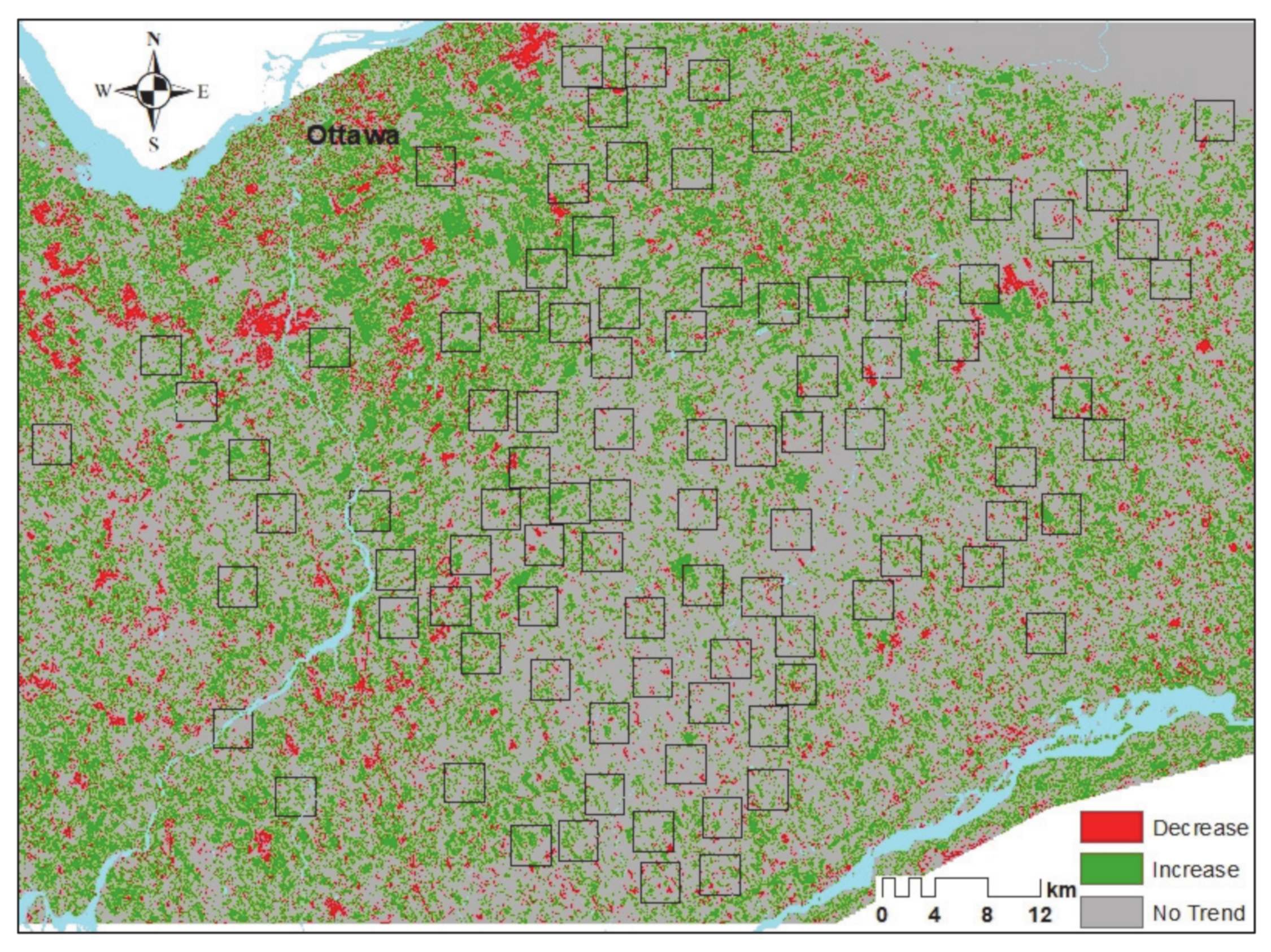
The evaluation of the TS slope and CMK significance for 2000–2011 July average MODIS NDVI data within the sample landscapes shows that 38% of all pixels demonstrated a statistically significant trend in NDVI. Many more pixels showed positive or negative trends that were not statistically significant [37]. Figure 2 shows the statistically significant positive (green) and negative (red) trends over the whole study region with the sample landscapes delineated. It is evident that there had been large areas of significant vegetation decline in the Ottawa region. This is generally due to urban development. These areas were not suitable for landscape selection because they were no longer completely agricultural in 2011–2012. Figure 3 displays close-ups of the results for three sample landscapes as an example. In Table 2, the percentage of pixels in each sample landscape that had significant negative or positive trends is shown as three groups (0%–4%, 5%–9%, and over 10%), along with the number of sample landscapes associated with each of these three groups. It is evident that more sample landscapes had greater proportions of pixels with significant positive trends in NDVI than negative trends. In particular, close to 1/3 of the sample landscapes (39 of 93) had more than 10% of their pixels showing a significant positive trend in NDVI over this period.
The results described above for MODIS NDVI data were more pronounced for the Landsat data, most likely because Landsat’s temporal archive (1985–2011) was longer than for MODIS. A larger proportion of Landsat pixels (48%) showed a significant trend (Figure 4), and many more sample landscapes had larger proportions of positively trending pixels than for the MODIS data (e.g., more than 10% of pixels demonstrated significant positive trends in 42% of the sample landscapes for the MODIS dataset and in 96% of the sample landscapes for the Landsat dataset, Table 2). Almost all sample landscapes (90 of 93) showed significant positive trends in more than 10% of their pixels, and the highest percentage of pixels in a sample landscape with a significantly positive trend was 45%. The MODIS data were somewhat better at detecting larger area positive NDVI trends associated with crop fields, particularly in large fields. Overall, the Landsat data were found to be much better for the detection of vegetation trends within the 3 × 3 km sample landscapes of this study; MODIS data would be appropriate for more generalized detection of trends over larger spatial extents.

3.2. Detection of a Change in Trend Slope for Subperiods in the Landsat Time Series

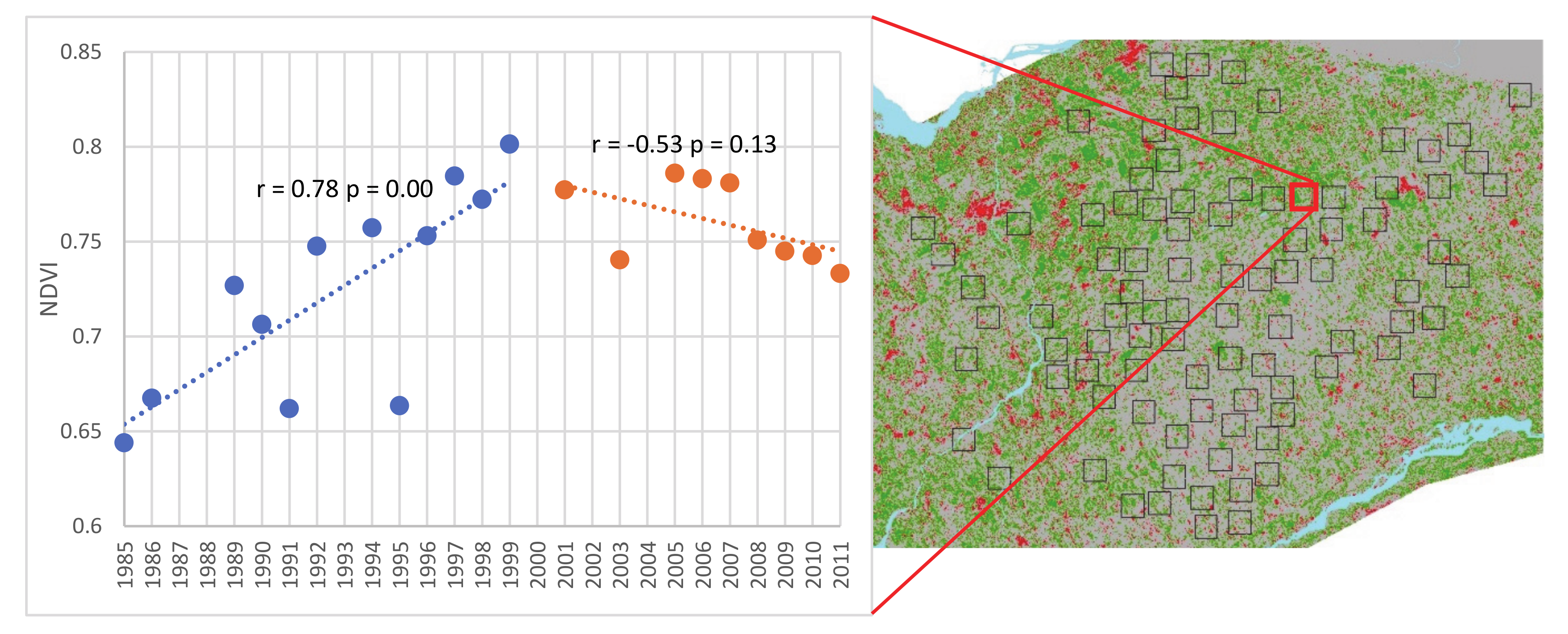
As a consequence of the analysis of the spatial average of the Landsat NDVI data for each sample landscape over the full 1985–2011 period, it was observed that more than half the sample landscapes (56 of 93) demonstrated a break in the time series and a change in the direction of the slope of the trend line from positive in the earlier subperiod to a non-significant or sometimes significantly negative slope in the later subperiod. This break was most evident for these sample landscapes for the subperiods of 1985–2000 and 2000–2011, although in some sample landscapes, later years such as 2005 were stronger breakpoints. An example of one sample landscape (coded H_L_40) is presented in Figure 5. Given this observed change in trend slope, and that the year 2000 was also the start of the MODIS time series, these two time periods were selected to compare the early versus late trends in Landsat NDVI and to compare Landsat and MODIS trends for all sample landscapes.
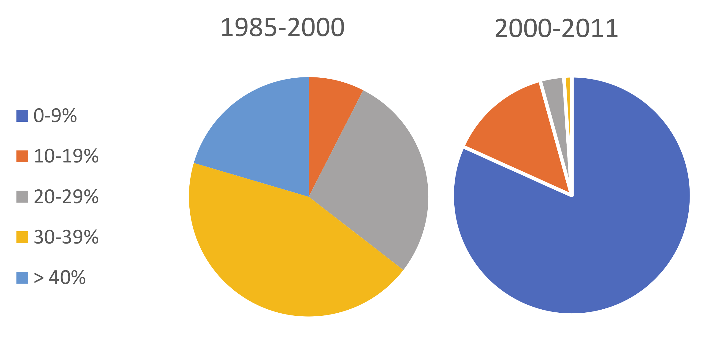
Comparing CMK significance for all pixels over all the 93 sample landscapes for 1985–2000 and 2000–2011 revealed that many more pixels displayed a positive trend in the earlier period compared to the later period. Figure 6 displays these results for both periods as five groupings, from 0–9% to over 40% of all pixels over all sample landscapes. Analysis at the landscape level showed that, for 1985–2000, the number of sample landscapes with a given percentage of pixels showing significant positive trends was as follows: 0%–19%—seven sample landscapes; 20%–29%—26 sample landscapes; 30%–39%—41 sample landscapes; > 40%—19 sample landscapes. The highest percentage of significantly positive trending pixels in a sample landscape was 58%. In contrast, for 2000–2011, only 17 sample landscapes had more than 10% of their pixels, showing a significant positive trend (highest percentage for a sample landscape was 33.5%). Negative trending pixels were far fewer, being less than 5% in all the sample landscapes for both periods. These results indicate that most sample landscapes showed distinct positive trends in vegetation productivity in up to 58% of their pixels during the earlier period, while in the later period, these trends leveled off to become non-significant, or for a small number of pixels in the given sample landscapes, NDVI declined.
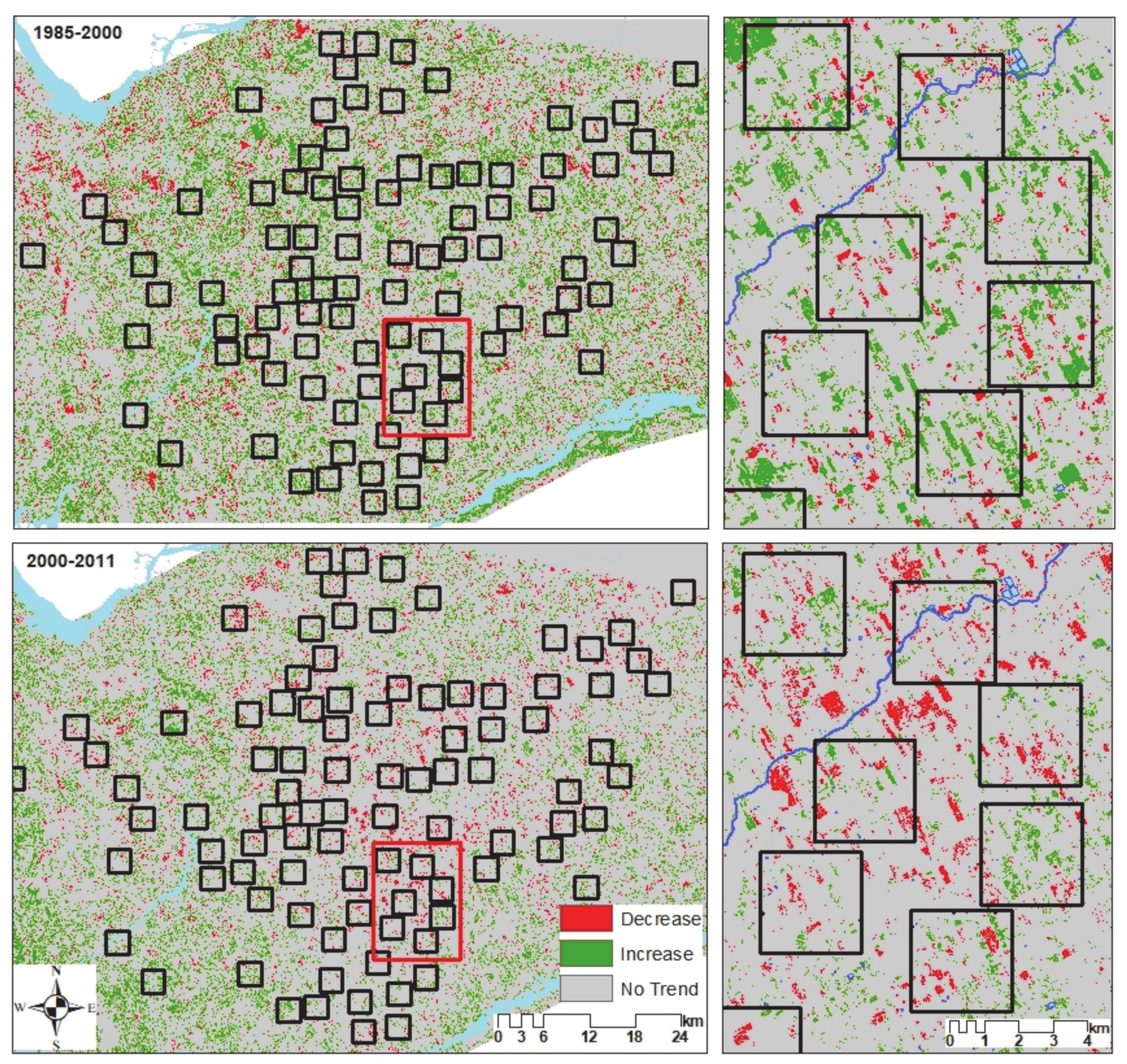
Figure 7 shows the results in map form for significant positive and negative trends over the whole study region and for some sample landscapes as an example. The total number of pixels over all the sample landscapes that displayed a significant negative slope was small in both periods but greater in the later period than in the earlier period.
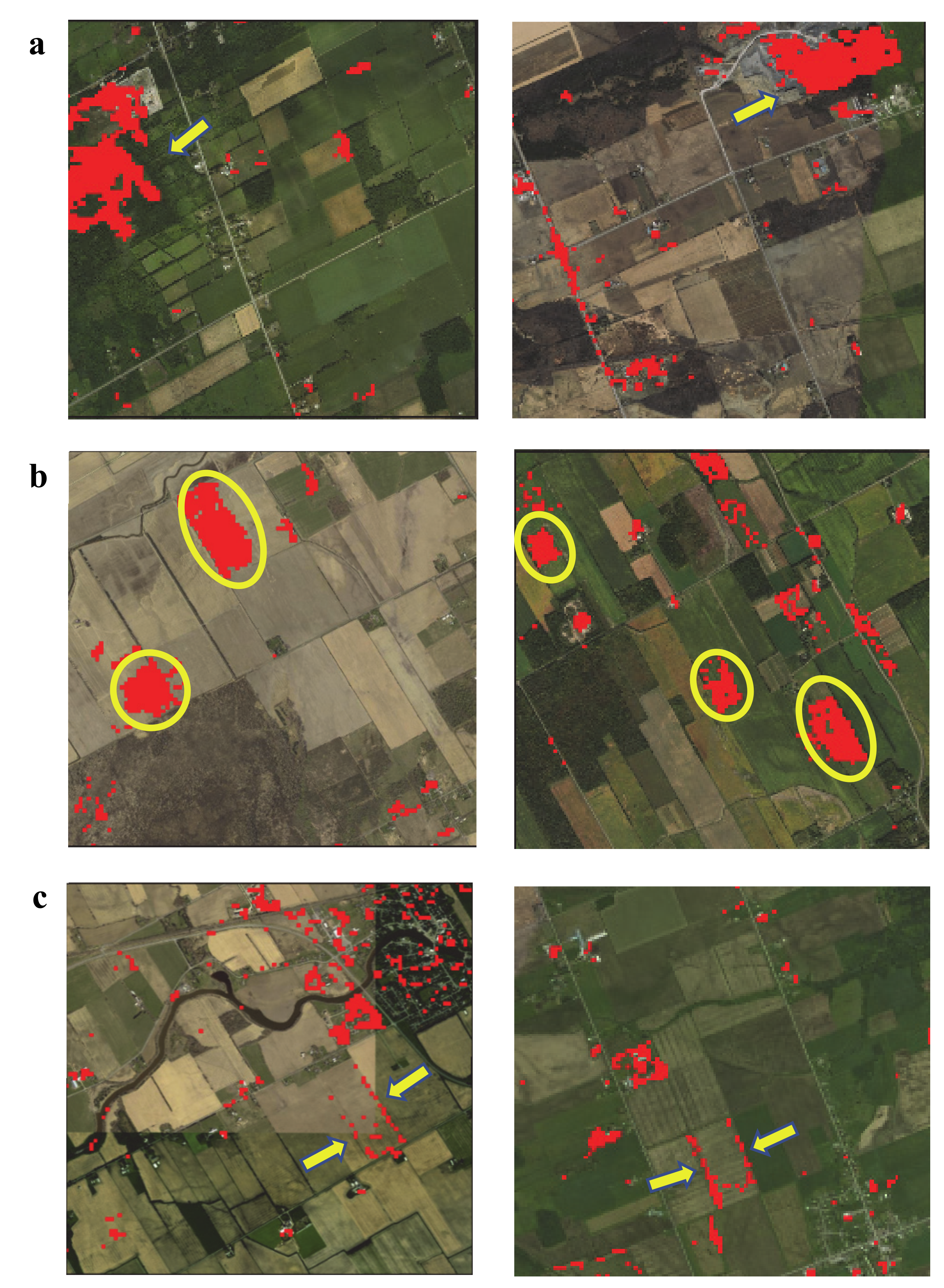
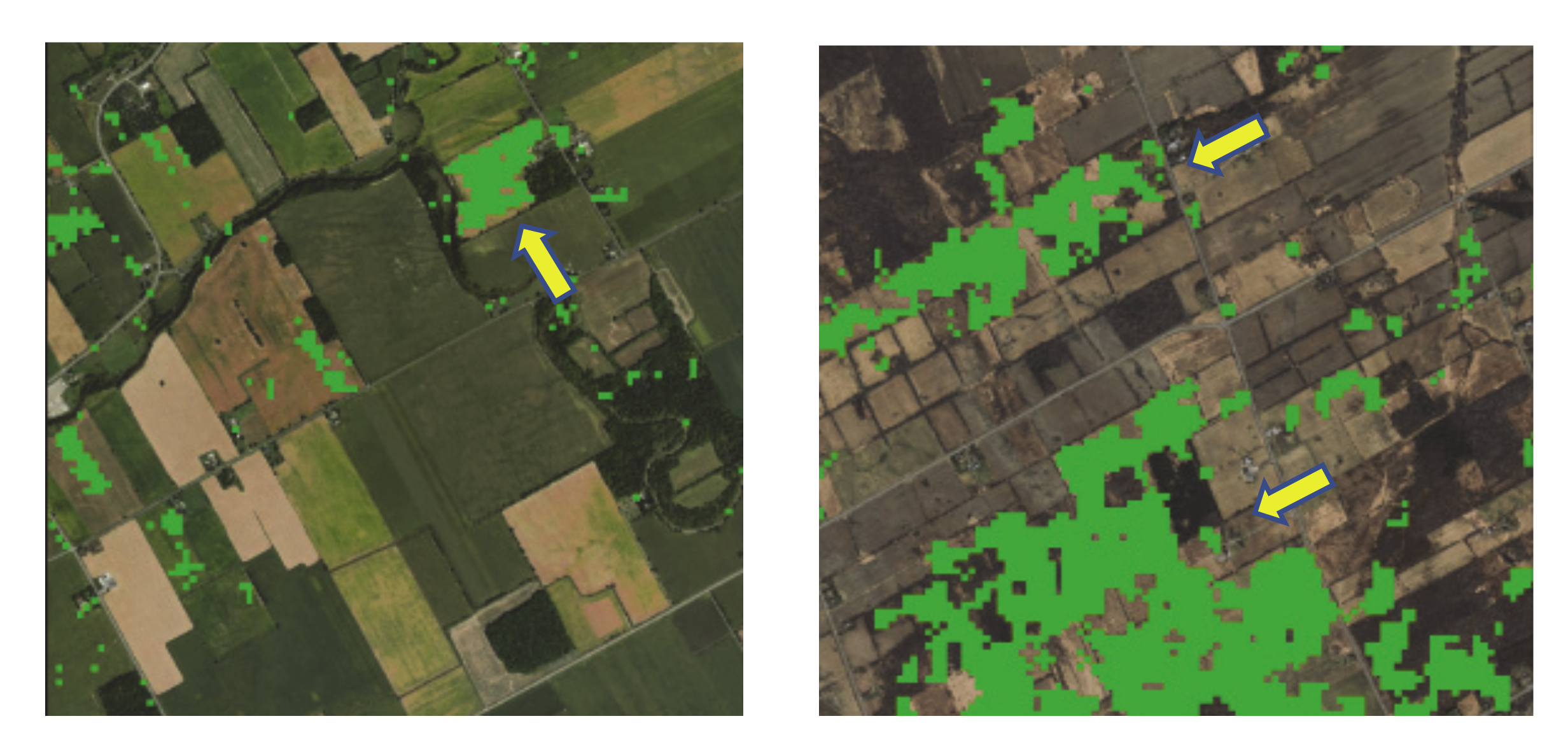
The negatively trending pixels in 2000–2011 were often associated with the removal of natural and semi-natural patches of trees or hedgerows (Figure 8). This was visually validated using of high resolution Google Earth imagery. In addition, most of the positive trends were associated with cropped lands, indicating increased green vegetation (Figure 9). This might be due to changes in agricultural practices or in landcover from crops with lower mid-summer NDVI to crops with higher mid-summer NDVI.

3.3. Comparing 2000–2011 MODIS and Landsat Mid-Summer NDVI Trends

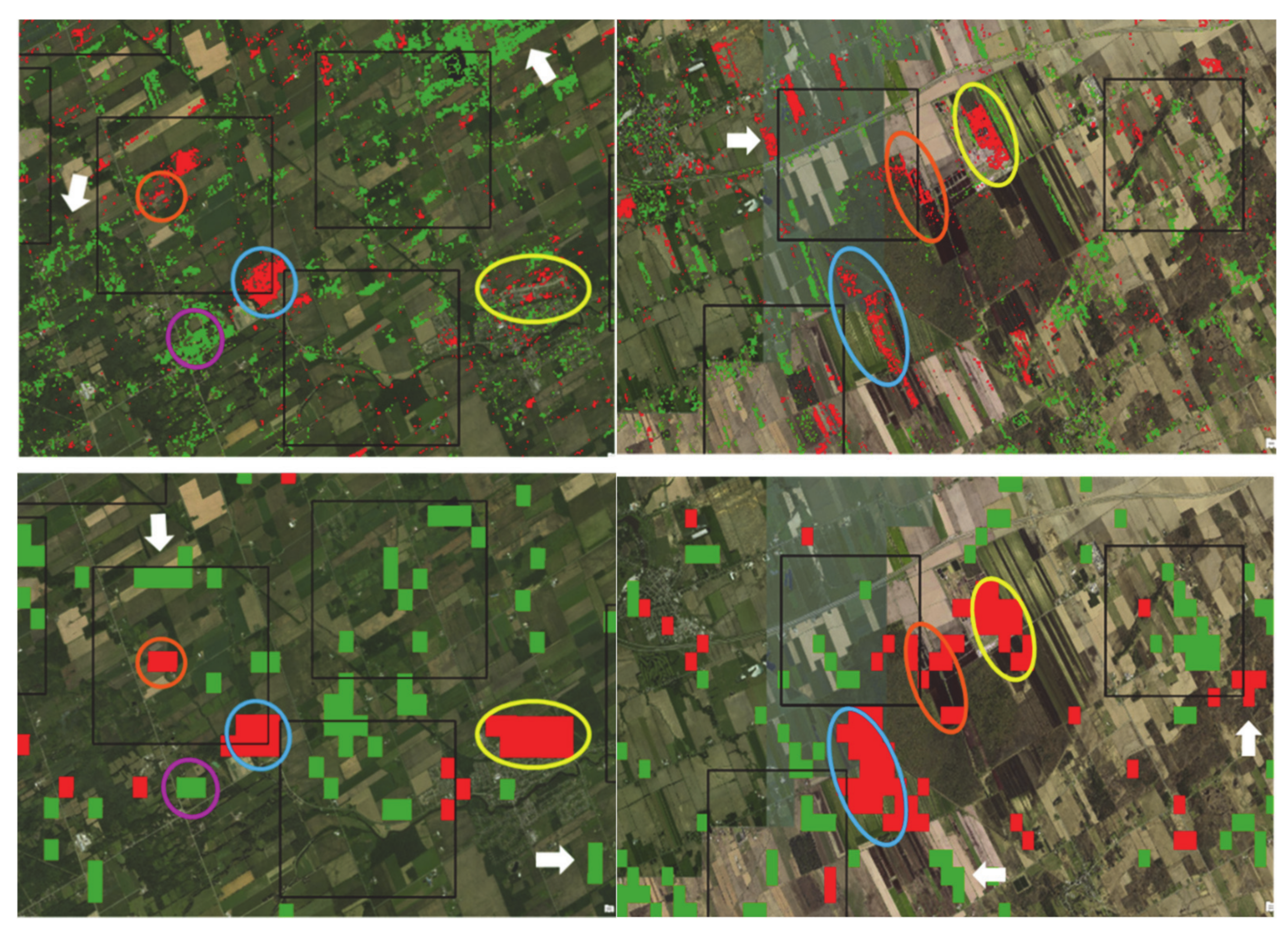
The cross-tabulation of the re-sampled MODIS 2000–2011 trend maps with their corresponding Landsat trend maps found that 92% of the MODIS pixels showing no trend were in agreement with those of Landsat, and 88.4% of Landsat pixels with no trend were in agreement with those of MODIS. However, only 3.1% of the MODIS significant negative trending pixels and 6.3% of the MODIS significant positive trending pixels were in agreement with the coincident Landsat pixels, and only 6.3% of the Landsat significant negative pixels and 8% of Landsat significant positive pixels were in agreement with the coincident MODIS pixels (Table 3). Despite this, the general spatial distribution of these pixels coincided well in many areas. Landsat generally identified more pixels with significant positive or negative trends and provided more spatial detail. MODIS identified fewer areas of significant change, and the spatial extent of those change areas, was often over-estimated. Figure 10 shows two example areas with spatially concurrent significant trends in both datasets as ellipses, while areas with significant trends identified by only one dataset are indicated by arrows. This figure also shows that Landsat pixels with significant trends are more spatially precise since they mostly fall within the boundaries of a given vegetation unit (field, forest, etc.). The coarse MODIS pixels often extended outside such boundaries in areas where change had not occurred, and they often extended outside the given sample landscape.
Overall, the Landsat data were found to be much better for the detection of vegetation trends within the 3 × 3 km sample landscapes. MODIS data were somewhat better at detecting larger area positive NDVI trends associated with crop fields, particularly in large fields, and such data would be appropriate for more generalized detection of vegetation trends over larger spatial extents than the 3 × 3 km landscapes of this study.

3.4. Modeling the Relationships of Biodiversity and Inter-Annual Landscape Dynamics

3.4.1. Relationships between Biodiversity and the Percentage of Sample Landscape Pixels with Significant Positive or Negative Trends in Vegetation Productivity

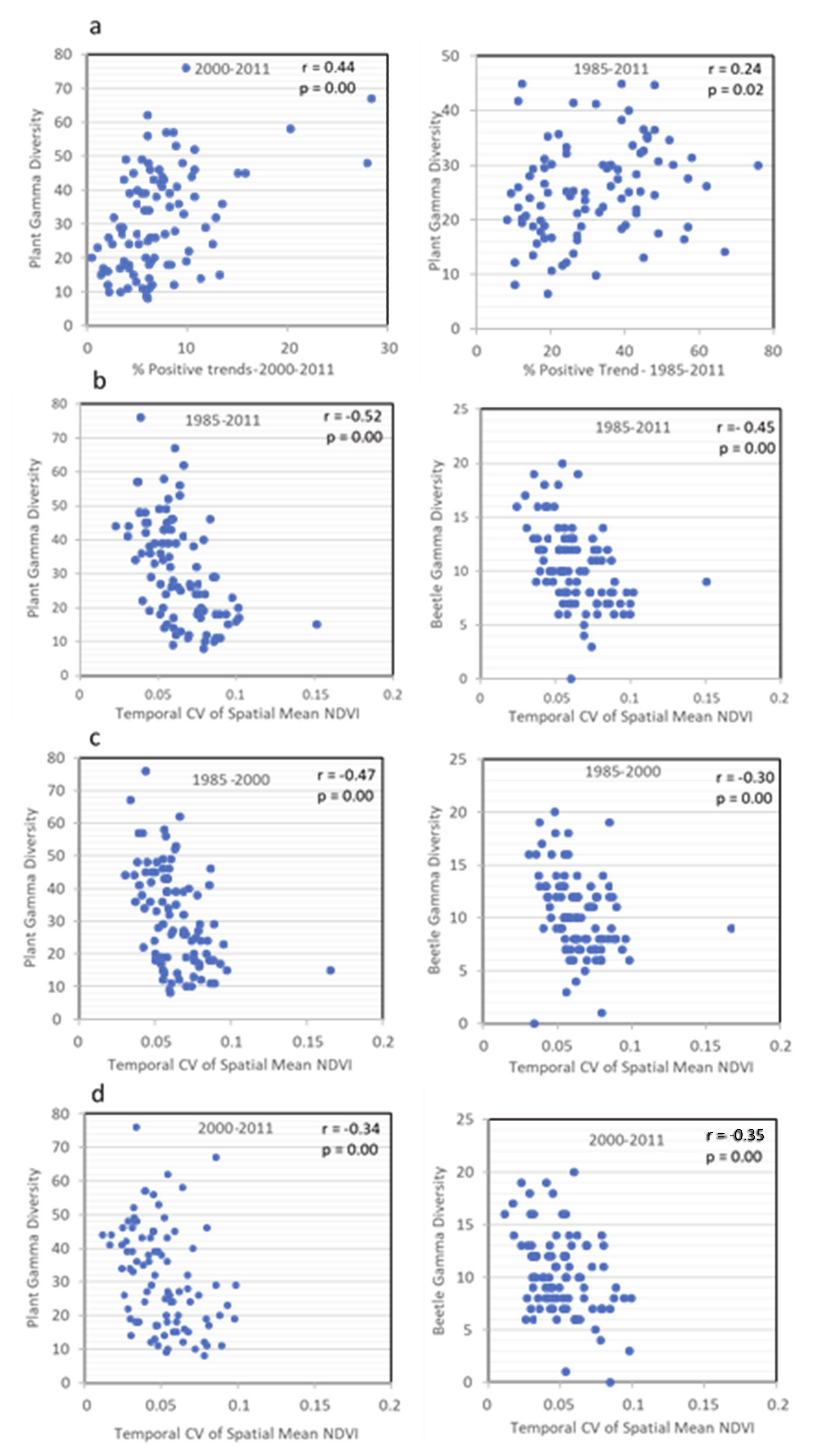
The relationships between the percentage of all pixels in a given sample landscape with a significant negative or positive inter-annual NDVI trend and 2011–2012 plant, beetle, bird, and butterfly gamma diversity were tested independently for the periods 2000–2011 (MODIS and Landsat), 1985–2000 (Landsat), and 1985–2011 (Landsat). No significant relationships were found for MODIS (2000–2011) nor for Landsat for the 1985–2000 period. However, for Landsat, the 2011–2012 plant diversity was positively related to the percentage of pixels in the sample landscapes with a significant positive trend in the 2000–2011 period (r = 0.44, p = 0.00) and over the entire temporal extent of 1985–2011 (r = 0.24, p = 0.02) (Figure 11). In Figure 11a (left), there are three distinct sample landscapes separate from the other data points at the upper end of the models; these sample landscapes had more than 20% of their pixels with significant positive NDVI trends. Removal of these three points reduced the correlation, but it was still significant (r = 0.33, p = 0.00); hence, these sample landscapes were not deemed to have a dominating effect on the relationship found.
Overall, these results show that where there was a gradual but significant increase in vegetation productivity during 2000–2011, plant species diversity measured over the sample landscapes at the end of this period was higher. This indicates that it is the decade preceding the biodiversity measurements that is more important than the decade before that in influencing biodiversity. The 17 sample landscapes with 10%–33.5% pixels having significant positive NDVI trends in 2000–2011 are important in the model showing increasing 2011–2012 plant biodiversity with such positive NDVI trends in the preceding decade.

3.4.2. Relationships between Biodiversity and Inter-Annual Variability in Vegetation Productivity

In biodiversity modeling using the inter-annual variability of NDVI at the landscape level (as represented by the temporal CV of the mean sample landscape NDVI and of the spatial CV of each sample landscape), no significant relationships were found for the MODIS data. Significant negative relationships (p < 0.01) were found between the 2011–2012 plant and beetle gamma diversity and Landsat temporal CV of the mean sample landscape NDVI for all the three-time periods as follows (Figure 11b–d): 1985–2011 (r = −0.52 (plants) and r = −0.45 (beetles); 1985–2000 (r = −0.47 (plants) and r = −0.30 (beetles), and 2000–2011 (r = −0.34 (plants) and r = −0.35 (beetles)). These results show that sample landscapes with higher antecedent inter-annual variability in average landscape vegetation productivity had lower 2011–2012 plant and beetle gamma diversity. For plants, this complements the result of Section 3.4.1, showing significant models for the proportion of pixels in each sample landscape with significant positive trends for the period 2000–2011. The relationships for both plants and beetles were stronger using the 1985–2011 data compared to the early and late periods independently, probably due to the longer period and more sample points (CV being sensitive to the number of samples) compared to each of the sub-periods.

3.4.3. Multiple Regression of Plant Gamma Diversity vs. Landscape Temporal Dynamics Metrics

Plants were the only taxon that demonstrated a significant relationship of gamma diversity with both types of temporal variables (temporal CV of the mean sample landscape NDVI; the percentage of significant positively trending pixels in each sample landscape), and this occurred for the 2000–2011 Landsat NDVI time series. The plant gamma diversity of 2011–2012 was, therefore, used in an SWR model against these two 2000–2011 temporal variables to test the relative importance of each variable in the model. These variables were not correlated with each other (r = −0.31) so multicollinearity was not an issue.
The resulting two-variable model demonstrated a stronger relationship (Adjusted R2 = 0.25, p = 0.00) than the best single variable model R2 for the 2000–2011 period. The percentage of significant positive trended NDVI pixels was the first variable entered (r = 0.44), while the temporal CV of the mean sample landscape NDVI was the second variable entered (r = −0.27). The results show that both temporal variable types are complementary, and, together, they strengthen the evidence of the initial hypothesis that temporal vegetation dynamics prior to a given year when biodiversity is assessed are significantly related to and potentially have an impact on biodiversity.

4. Discussion

This study had two main components: 1) detect and evaluate temporal trends in vegetation productivity in agricultural landscapes of eastern Ontario during the years preceding 2012 using MODIS and Landsat data, and 2) determine if these vegetation dynamics are related to farmland biodiversity measured in 2011–2012.

4.1. Trends in Vegetation Productivity

Significant positive trends in the mid-summer NDVI data were found in all sample landscapes with the proportion of pixels showing such trends being over 1/3 for MODIS (2000–2011) and almost ½ for Landsat (1985–2011). Most of these trends occurred in the cropped portion of the sample landscapes, indicating increased green vegetation due either to agricultural practices or changes from crop types, such as alfalfa and winter wheat, which are harvested in this region in summer, to denser foliage crops such as corn and soybean; demand for the latter two crops increased in the last two decades for feed (both) and ethanol fuel (corn) [46]. According to the Census of Agriculture produced by Statistics Canada [2], a major shift in crop composition in Ontario in the early 2000s was reported from less heavily managed crops such as hay, alfalfa, and perennial plants to more intensively managed crops such as corn and soybean. These positive trends were most evident in low heterogeneity sample landscapes with few crop types and large fields [37].
While the percentage of pixels showing significant negative trends in sample landscapes was smaller, those pixels were often spatially clustered and associated with the removal of woody vegetation or destruction of natural patches for either crop production or new buildings. Higher proportions of pixels in sample landscapes with high compositional heterogeneity (more crop types) and configurational heterogeneity (smaller field sizes), both of which are known to benefit biodiversity [20], showed negative trends in vegetation productivity [37] in a general process of agricultural intensification over the study period. The detection of smaller negative trending areas within sample landscapes was facilitated much better using the higher spatial resolution Landsat data. Although up to 144 MODIS pixels overlapped with each sample landscape (depending on pixel alignment and image orientation with respect to sample landscape orientation), at 250 m pixel spacing, they were too large to consistently detect removal of trees and hedgerows. This concurs with Rogers et al. [47] who found coarser spatial resolution AVHRR and MODIS time series to be poorer than Landsat time series in portraying temporal changes and detecting early signs of tree mortality in the boreal forests of North America.
Additionally, during 1985–2000, many Landsat pixels in the sample landscapes demonstrated significant positive trends while between 2000 and 2011, many pixels demonstrated no trend or a significant negative trend. The analysis of such sub-periods could be extended to shorter intervals (e.g., 2–4 years) to evaluate the effects of crop rotation, other landscape changes, or short-term weather variations. Different time intervals could be selected to test the effect of time series length on the trends, to identify different sub-trends, and to test the sensitivity of trends to the selected time intervals between images. For example, Czerwinski et al. [44] divided a 20-year time series of Landsat 5 images into 1–3, 4–5, and 6–7 year intervals to analyze time series extent effects on the detection of forest changes, finding that the 1–3 and 4–5 year intervals produced similar change results, while the 6–7 year interval did not detect the same changes and suggested very little changes had occurred.

4.2. Relationships of Biodiversity with Inter-Annual Landscape Vegetation Dynamics

As for the trend analysis, Landsat data were much better for modeling biodiversity than MODIS data (which did not produce any significant models). For Landsat data, plant gamma diversity measured in 2011–2012 was found to be negatively related to the temporal variability (CV) in NDVI during the preceding 26 years, as well as for the two sub-periods of 1985–2000 and 2000–2011. Plant diversity was also positively related to the proportion of pixels with a significant positive trend for 2000–2011 and 1985–2011 in each sample landscape. However, this relationship was stronger in 2000–2011 compared to 1985–2011, indicating that a more recent trend in vegetation may have a stronger influence on plant diversity. In the stepwise regression, a two-variable model for plant diversity was derived with the percentage of pixels with a significant positive NDVI trend accounting for more variance than the inter-annual variation (CV) in NDVI. These results for plants were generally as expected. In sample landscapes with more pixels showing a long-term increase in vegetation quantity and where inter-annual variability in vegetation quantity is lower (i.e., less year-to-year variability in NDVI), more wild plant species could be established. For beetles, higher inter-annual variation in vegetation quantity was also associated with reduced gamma diversity. Most of the beetle species surveyed prefer vegetated habitats. Therefore, high inter-annual variation in the mid-summer vegetation quantity, where in some years vegetation is thinner with greater soil exposure due to weather, the selected crop type, and phenology, or other management practices, results in lower beetle diversity.
Despite being statistically significant, these relationships account for low amounts of variance in gamma diversity, i.e., they are noisy. This may be because a process such as agricultural intensification that has occurred within the study area during the decades of the data used for this study may have contrasting effects. The relationships found indicated that a greater proportion of pixels with positive long-term NDVI trends in a sample landscape is associated with higher plant diversity, and this trend in sample landscapes is most likely due to transitions to higher biomass crops such as corn and soybeans. However, through such intensification, many farms have also experienced the removal of natural vegetation in woodlots and at field boundaries, which reduces landscape NDVI, while herbicide use increases, directly killing off some non-crop plant species. The former increases noise in the x-variable (% pixels with significant positive trend) while the latter increases noise in the y-variable (plant gamma diversity). The relationships found here are, therefore, not appropriate for the prediction of biodiversity, but they do give statistical evidence that plant and beetle diversity are related to vegetation trends over the long-term as well as inter-annual vegetation dynamics. This is important new knowledge with respect to the development of an understanding of impacts of farming on biodiversity in the temporal dimension; it is complementary to the multitude of studies that have shown impacts of landscape spatial heterogeneity on biodiversity.
This is one of the first, or the first study evaluating effects of such temporal trends and inter-annual vegetation dynamics on biodiversity in agricultural landscapes using remote sensing time-series data. Previous studies found negative impacts of agricultural land use change. For instance, Senapathi et al. [23] used digitized land cover maps to assess the impacts of 80 years of land cover change on bee and wasp species richness and community composition in England. Reidsma et al. [22] used the European Union Farm Accountancy Data Network to classify different farm types and land use intensity, and assessed and projected the impacts of agricultural land use change on biodiversity for 2010, 2020, and 2030 scenarios. Jiang et al. [21] used data from the ground sampling of three sites with different land use practices to assess the impact on plant species richness. However, remote sensing-based time series data were not utilized in those studies and, therefore, studies in other environments and contexts were consulted for comparison. At broader scales, De Baan et al. [48] found generally negative impacts of change in different land use types on biodiversity in various regions of the earth. Jetz et al. [49] estimated the projected impacts of climate change and land use change on global avian diversity and found that 400 species are projected to suffer by the year 2050. Such studies have a temporal dimension but generally use land cover maps created for one or more years instead of a time series of remotely sensed reflectance data, as in this study.

4.3. Limitations and Recommendations for Future Research

This study was constrained by the biodiversity data, which were acquired in 2011–2012 as part of a large field and remote sensing project (e.g., [20,33,36] amongst others). The acquisition of the biodiversity data was a major undertaking by teams of up to 10 field personnel over the April–September period in both years (1/2 the sample landscapes surveyed in each year). The use of such intensive and directly acquired biodiversity data provides an excellent reference for such remote sensing modeling studies. However, being essentially at one point in time limits such a temporal study as this to the analysis of the potential effects of antecedent vegetation dynamics on biodiversity measured at that time. While the results of this study are illuminating and point to the potential impacts of temporal landscape dynamics on farmland biodiversity, better temporal biodiversity data could be pursued, using continuous multi-year field efforts. In fact, a portion of the sample landscapes of this study were revisited in 2016, and 2017 and bee and butterfly species were surveyed using the same protocols by a field crew in the Landscape Science and Technology Division in Environment and Climate Change Canada [50]. The sample landscapes may be visited in the future and used as long-term monitoring sites to assess the effects of changes in the landscape as well as climate factors on pollinator diversity in Eastern Ontario. In addition, other biodiversity indicators may be acquired over a given time period. However, Hanley et al. [4], in a study using density-based metrics and species richness in models based on farm types with various land uses (e.g., grazing and sheep, dairy, and beef production), management practices and policy scenarios, caution on using umbrella species or generalized biodiversity indicators such as total richness, which can miss important species compositional effects. Sources such as the long-term USGS North American Breeding Bird Survey [51] are recommended for use as a temporal reference dataset for modeling against landscape dynamics as derived from remote sensing time series. In addition, comparing farmland biodiversity with the biodiversity of adjacent natural and semi-natural lands is recommended to assess the changes in species diversity due to land conversion to agriculture.
With respect to the remote sensing data used in this study, the coarse spatial resolution of the MODIS data was expected to be a hindrance in trend analysis and biodiversity modeling in comparison to Landsat data for the given landscape scale. However, its excellent temporal resolution allowed better temporal precision of average mid-summer NDVI estimation than for Landsat, where single images had to be used that varied in acquisition date, potentially adding noise to the trends and biodiversity models. Thus, MODIS is more useful for larger regional or global inter- and intra-annual trend analysis, as others have found. Alternatively, fusion techniques could be investigated to take advantage of the MODIS high temporal resolution and Landsat high spatial resolution (e.g., [52,53,54] in studies of landscape changes and trends). High-resolution image time-series data from other sensor platforms (e.g., air photos; Quickbird-Worldview) were not archived for the study area and would have been very costly to acquire over the spatial and temporal extents of this study. Where the resources exist to acquire such data over both a suitably long period and with sufficient areal coverage to represent a given eco-zone (such as the farmland region of this study), future research should consider such data. They should be able to detect smaller areas of vegetation trends with better spatial precision than Landsat, and some taxa may respond to such small vegetation changes. However, many or most species in the four taxa of this study are known to function and disperse over larger areas (e.g., by flight or wind), so it is uncertain if higher-resolution detection of vegetation trends and variability in small areas would improve such biodiversity modeling. Such data could be used to try to determine the scale of the effects of vegetation dynamics on biodiversity to see if there are differences among taxa. This is an interesting question that we could not tackle with our datasets. In addition, comparison of LULC classifications derived from such high-resolution imagery over time could aid in the identification of the causes of the detected vegetation trends and variability, provided error propagation is not significant as discussed in the Introduction. Analysis of patch-based metrics derived from such maps may help elucidate processes such as changes in connectivity over time that could affect the biodiversity of certain species or taxa. These could be useful in guiding the development of policy and guidelines regarding farmland management over time for the enhancement of the diversity of given taxa.

4.4. Implications of This Study for Policy and Monitoring of Biodiversity

In the past few decades, Canadian agricultural policy has shifted from increasing output and promotion of income stability in the agriculture sector to research focusing on sustainable ways to increase productivity and limit environmental impacts [55]. To fulfill this, Agriculture and Agri-food Canada (AAFC) uses a series of agri-environmental indicators in the analysis of overall environmental performance. These indicators are assessed over time, and areas showing improvements are highlighted, while regions that require policy interventions are identified. For example, the Wildlife Habitat on Farmland Index [55], as an indicator of biodiversity, demonstrated a decline from a “moderate’ state in 1986 to a “poor” state in 2011 in Canada.
Indices such as this that are developed and employed at the national or provincial level are often based on mapping of habitat using field observations and classification of moderate to coarse resolution remote sensing imagery. Given that comparison of classifications from different years and over a time series is sensitive to error propagation as mentioned previously, aggregated amounts of ‘habitat’ are often generated by year and compared between years, as opposed to specific statistics on class trends and changes from one class to another. The main advantage of the methods of this study is that they do not require such a classification step and avoid the associated map error propagation in the time series analysis. The methods of this study could be automated and used operationally to evaluate vegetation productivity trends and variability as a type of index of potential biodiversity (at least for plants and beetles, as shown here). In addition, a hybrid of the classification and reflectance approaches could also be developed, for example, by delineating areas of significant NDVI trends or high variability using segmentation. Indices of the abundance and spatial properties (e.g., fragmentation, connectivity metrics) of these identified patches could then be derived and used in more detailed landscape vegetation and habitat analysis that feed into policy interventions of the type mentioned above for AAFC. The demonstration and justification to farmers of the value of maintaining stable crop field vegetation cover from year to year and the preservation or installation of natural and seminatural vegetation are suggested as means to enhance farmland biodiversity and reinforce such agricultural policies.

5. Conclusions

This study evaluated relationships between long-term farmland temporal vegetation productivity dynamics and 2011–2012 biodiversity of four taxa (plants, beetles, birds, and butterflies). It compared the potential of MODIS and Landsat 2000–2011 time-series datasets, as well as Landsat for the additional periods of 1985–2000 and 1985–2011, in detecting significant positive or negative trends in NDVI in 93 sample landscapes of 3 x 3 km in a predominantly agricultural area of eastern Ontario. Over all sample landscapes, 38% of MODIS (2000–2011) pixels, and 48% of Landsat (1985–2011) pixels showed significant positive or negative NDVI trends, with positive trends being more dominant than negative trends. Most of the significant negative trends were spatially associated with removal of natural and semi-natural patches, and, in some cases, the removal of field edges and hedgerows, and these were better detected with the higher resolution Landsat data. The most significant positive trends in NDVI were in crop fields and probably associated with increasing crop density, either by changes in crop type over time or by management practices to increase growth and yield. The full 1985–2011 period of Landsat data showed a break in the slope of NDVI about the year 2000 for many sample landscapes where a positive slope from 1985–2000 changed to a non-significant or, in some cases, a negative slope for 2000–2011.
While MODIS data did not produce significant models of biodiversity, using Landsat data, the proportion of sample landscape pixels with significant positive trends and the inter-annual variation (CV) of the mean sample landscape NDVI were significantly related to the 2011–2012 gamma diversity of plants (positively and negatively, respectively). For beetles, gamma diversity was also significantly and negatively related to the temporal CV of the mean sample landscape NDVI. The relationships for the CV of NDVI were stronger for the overall Landsat data period (1985–2011) than for either of the sub-periods of 1985–2000 and 2000–2011. In future work, higher resolution airborne or satellite image time series, if available and affordable for a long-term regional study such as this, would help identify smaller areas of vegetation dynamics that may be more strongly associated with species and taxa life cycle functions, thereby potentially providing stronger biodiversity models.
Besides this study, the effects of inter-annual changes in remote sensing-based agricultural landscape vegetation indices on biodiversity have not been largely studied. The results found here show that long-term trends and inter-annual vegetation variability are complementary indicators of the potential effects on farmland biodiversity and can be used to inform landscape management policy and practice. This study has also demonstrated the value of remotely sensed reflectance time series data in the detection of vegetation trends and the modeling of biodiversity. This approach is a viable and simpler alternative to the classification and temporal thematic map comparison analysis. It depends only on well-calibrated reflectance data time series, which are freely available for several sensors, in contrast to temporal analysis of thematic classifications, which is highly sensitive to error propagation. Further research is warranted using other temporal analysis techniques and additional temporal metrics as well as temporal biodiversity datasets.

Author Contributions

This research was designed jointly by N.A. and D.K. N.A. performed the experiments and analysis, wrote the first draft of the paper, and drafted the revisions. D.K. reviewed and edited the paper drafts, contributed to the paper revisions, and provided advice on research design, implementation, and paper content. All authors have read and agreed to the published version of the manuscript.

Funding

This research was funded by the National Sciences and Engineering Council (NSERC) through: (1) a Strategic Project Grant to L. Fahrig, D. King, and S. Mitchell of Carleton University, and K. Lindsay of Environment and Climate Change Canada, and (2) a Discovery Grant to D. King. Environment and Climate Change Canada provided additional funding through a Grants and Contributions Agreement with Fahrig, King, Mitchell and Lindsay.

Acknowledgments

The authors are very grateful for the advice of Scott Mitchell of the Department of Geography and Environmental Studies, Carleton University. They also would like to thank Earth Observation (STB-EO) team at Agriculture and Agri-food Canada, Science, and Technology Branch, especially Andrew Davidson, Catherine Champagne, and Laura Dingle Robertson for providing the MODIS data and relevant technical tools for this research. They would also like to express deep appreciation to the Geomatics team at Landscape Science and Technology Division (LSTD) Environment and Climate Change Canada, especially Darren Pouliot, for providing the technical tools and valuable comments and Jason Duffe for supporting the time and resources to write this paper.

Conflicts of Interest

The authors declare no conflict of interest.

References

  1. Fahrig, L. Rethinking patch size and isolation effects: the habitat amount hypothesis. J. Biogeogr. 2013, 40, 1649–1663. [Google Scholar] [CrossRef]
  2. 2016 Census of Agriculture. Available online: https://www.statcan.gc.ca/eng/ca2016 (accessed on 4 November 2018).
  3. Norris, K. Agriculture and biodiversity conservation: opportunity knocks. Conserv. Lett. 2008, 1, 2–11. [Google Scholar] [CrossRef]
  4. Hanley, N.; Acs, S.; Dallimer, M.; Gaston, K.J.; Graves, A.; Morris, J.; Armsworth, P.R. Farm-scale ecological and economic impacts of agricultural change in the uplands. Land Use Policy 2012, 29, 587–597. [Google Scholar] [CrossRef]
  5. Environmental sustainability of Canadian Agriculture: Agri-Environmental Indicator Report Series-Report #4. Available online: http://www.agr.gc.ca/eng/agriculture-and-climate/agricultural-practices/environmental-sustainability-of-canadian-agriculture-agri-environmental-indicator-report-series-report-4/?id=1467307820931 (accessed on 25 December 2018).
  6. Yeates, G.W.; Bardgett, R.D.; Cook, R.; Hobbs, P.; Bowling, P.; Potter, F. Faunal and microbial diversity in three Welsh grassland soils under conventional and organic management regimes. J. Appl. Ecol. 1997, 34, 453–470. [Google Scholar] [CrossRef]
  7. Hansen, B.; Fjelsted, H.; Kristensn, S. Approaches to assess the environmental impact of organic farming with particular regard to Denmark. Agr. Ecosyst. Environ. 2001, 83, 11–26. [Google Scholar] [CrossRef]
  8. Hald, A.B. Weed vegetation (wild flora) of long established organic versus conventional cereal fields in Denmark. Ann. Appl. Biol. 1999, 134, 307–314. [Google Scholar] [CrossRef]
  9. Benton, T.; Vickery, J.A.; Wilson, J.D. Farmland biodiversity: Is habitat heterogeneity the key? Trends Ecol. Evol. 2003, 18, 182–188. [Google Scholar] [CrossRef]
  10. Farhig, L.; Baudry, J.; Brotons, L.; Burel, F.G.; Crist, T.O.; Fuller, R.J.; Sirami, C.; Siriwardena, G.M.; Martin, J.L. Functional landscape heterogeneity and animal biodiversity in agricultural landscapes. Ecol. Lett. 2011, 14, 101–112. [Google Scholar]
  11. Freemark, K.; Boutin, C.; Keddy, C. Importance of farmland habitats for conservation of plant species. Conserv. Biol. 2002, 16, 399–412. [Google Scholar] [CrossRef]
  12. Flick, T.; Feagan, S.; Fahrig, L. Effects of landscape structure on butterfly species richness and abundance in agricultural landscapes in eastern Ontario, Canada. Agr. Ecosyst. Environ. 2012, 156, 123–133. [Google Scholar] [CrossRef]
  13. Zamora, J.; Verdu, J.R.; Eduardo, G. Species richness in Mediterranean agroecosystems: Spatial and temporal analysis for biodiversity conservation. Biol. Conserv. 2007, 134, 113–121. [Google Scholar] [CrossRef]
  14. Kleijn, D.; Kohler, F.; Baldi, A.; Batary, P.; Concepcion, E.D.; Clough, Y.; Dıaz, M.; Gabriel, D.; Holzschuh, A.; Knop, E.; et al. On the relationship between farmland biodiversity and land-use intensity in Europe. In Proceedings of the Royal Society B: biological sciences; Royal Society B: London, UK, 2009; Volume 276, pp. 903–909. [Google Scholar]
  15. Krauss, J.; Bommarco, R.; Guardiola, M.; Heikkinen, R.K.; Helm, A.; Kuussaari, M.; Lindborg, R.; Öckinger, E.; Pärtel, M.; Pino, J.; et al. Habitat fragmentation causes immediate and time-delayed biodiversity loss at different trophic levels. Ecol. Lett. 2010, 13, 597–605. [Google Scholar] [CrossRef] [PubMed] [Green Version]
  16. Wagner, H.; Wildi, O.; Ewald, L. Additive partitioning of plant species diversity in an agricultural mosaic landscape. Landsc. Ecol. 2000, 15, 219–227. [Google Scholar] [CrossRef]
  17. Smart, S.; Bunce, R.; Firbank, L.; Coward, P. Do field boundaries act as refugia for grassland plant species diversity in intensively managed agricultural landscapes in Britain? Agr. Ecosyst. Environ. 2002, 91, 73–87. [Google Scholar] [CrossRef]
  18. Albrecht, M.; Peter, D.; Christine, M.; David, K.; Bernhard, S. The Swiss agri-environment scheme enhances pollinator diversity and plant reproductive success in nearby intensively managed farmland. J. Appl. Ecol. 2007, 44, 813–822. [Google Scholar] [CrossRef]
  19. Brose, U. Relative importance of isolation, area and habitat heterogeneity for vascular plant species richness of temporary wetlands in east-German farmland. Ecography 2001, 24, 722–730. [Google Scholar] [CrossRef]
  20. Fahrig, L.; Girard, J.; Duro, D.; Pasher, J.; Smith, A.; Javorek, S.; King, D.; Freemark Lindsay, K.; Mitchell, S.; Tischendorf, L. Farmlands with smaller crop fields have higher within-field biodiversity. Agr. Ecosyst. Environ. 2015, 200, 219–234. [Google Scholar] [CrossRef]
  21. Jiang, Y.; Kang, M.; Gao, Q.; He, L.; Xiong, M.; Jia, Z.; Jin, Z. Impact of land use on plant biodiversity and measures for biodiversity conservation in the Loess Plateau in China – a case study in a hilly-gully region of the Northern Loess Plateau. Biodivers. Conserv. 2003, 12, 2121–2133. [Google Scholar] [CrossRef]
  22. Reidsma, P.; Tekelenburg, T.; van den Berg, M.; Alkemade, R. Impacts of land-use change on biodiversity: An assessment of agricultural biodiversity in the European Union. Agr. Ecosyst. and Environ. 2006, 114, 86–102. [Google Scholar] [CrossRef]
  23. Senapathi, D.; Carvalheiro, L.G.; Biesmeijer, J.C.; Dodson, C.A.; Evans, R.L.; McKerchar, M.; Morton, R.D.; Moss, E.D.; Stuart, P.M.; Kunin, W.E.; et al. The impact of over 80 years of land cover changes on bee and wasp pollinator communities in England. In Proceedings of the Royal Society B: Biological Sciences; Royal Society B: London, UK, 2015; Volume 282, p. 20150294. [Google Scholar]
  24. Nagendra, H. Review article: Using remote sensing to assess biodiversity. Int. J. Remote Sens. 2001, 22, 2377–2400. [Google Scholar] [CrossRef]
  25. Nagendra, H.; Lucas, R.; Honradoc, J.P.; Adamo, M.; Mairota, P. Remote sensing for conservation monitoring: Assessing protected areas, habitat extent, habitat condition, species diversity, and threats. Ecol. Indic. 2013, 33, 45–59. [Google Scholar] [CrossRef]
  26. Turner, W.; Spector, S.; Gardiner, N.; Fladeland, M.; Sterling, E.; Steininger, M. Remote sensing for biodiversity science and conservation. Trends Ecol. Evol. 2003, 18, 306–314. [Google Scholar] [CrossRef]
  27. Franklin, S.E. Remote Sensing for Biodiversity and Wildlife Management: Synthesis and Applications; McGraw-Hill Education: Whitby, UK, 2009. [Google Scholar]
  28. Rocchini, D.; Balkenhol, N.; Carter, G.A.; Foody, G.M.; Gillespie, T.W.; He, K.S.; Kark, S.; Levin, N.; Lucas, K.; Nagendra, H. Remotely sensed spectral heterogeneity as a proxy of species diversity: Recent advances and open challenges. Ecol. Inform. 2010, 5, 318–329. [Google Scholar] [CrossRef]
  29. Kuenzer, C.; Ottinger, M.; Wegmann, G.H.; Wang, C.; Zhang, J.; Dech, S.; Wikelski, M. Review Article: Earth observation satellite sensors for biodiversity monitoring: potentials and bottlenecks. Int. J. Remote Sens. 2014, 35, 6599–6647. [Google Scholar] [CrossRef] [Green Version]
  30. Wilson, S.; Mitchell, G.W.; Pasher, J.; McGovern, M.; Hudson, M.A.R.; Fahrig, L. Influence of crop type, heterogeneity and woody structure on avian biodiversity in agricultural landscapes. Ecol. Indic. 2017, 83, 218–226. [Google Scholar] [CrossRef]
  31. Palmer, M.W.; Wohlgemuth, T.; Earls, P.G.; Arévalo, J.R.; Thompson, S. Opportunities for Long-Term Ecological Research at the Tallgrass Prairie Preserve, Oklahoma. In Proceedings of the ILTER Regional Workshop: Cooperation in Long Term Ecological Research in Central and Eastern Europe, Budapest, Hungary, 22 June 1999. [Google Scholar]
  32. Gillespie, T.; Foody, G.M.; Rocchini, D. Measuring and modelling biodiversity from space. Prog. Phys. Geogr. 2008, 32, 203–221. [Google Scholar] [CrossRef]
  33. Duro, D.; Girard, J.; King, D.; Fahrig, L.; Mitchell, S.; Lindsay, K.; Tischendorf, L. Predicting species diversity in agricultural environments using Landsat TM imagery. Remote Sens. Environ. 2014, 144, 214–225. [Google Scholar] [CrossRef]
  34. St-Louis, V.; Pidgeon, A.M.; Kuemmerle, T.; Sonnenschein, R.; Radeloff, V.C.; Clayton, M.K.; Locke, B.A.; Bash, D.; Hostert, P. Modelling avian biodiversity using raw, unclassified satellite imagery. Philos. Transl. R. Soc. B Biol. Sci. 2014, 369, 20130197. [Google Scholar] [CrossRef] [Green Version]
  35. Ontario Ministry of Agriculture, Food and Rural Affairs. Available online: http://www.omafra.gov.on.ca/english/crops/index (accessed on 18 October 2011).
  36. Pasher, J.; Mitchell, S.; King, D.; Fahrig, L.; Smith, A.; Lindsay, K. Optimizing landscape selection for estimating relative effects of landscape variables on ecological responses. Landsc. Ecol. 2013, 28, 371–383. [Google Scholar] [CrossRef]
  37. Alavi, N. Evaluating the Relationships of Phenological and Inter-Annual Landscape Dynamics with Farmland Biodiversity using Multi-Spatial and Multi-Temporal Remote Sensing Data. Ph.D. Thesis, Carleton University, Ottawa, ON, Canada.
  38. Crist, E. A TM Tasseled Cap Equivalent Transformation for Reflectance Factor Data. Remote Sens. Environ. 1985, 17, 301–306. [Google Scholar] [CrossRef]
  39. Theil, H. A rank-invariant method of linear and polynomial regression analysis. I, II, III. Nederl. Akad. Wetensch. Proc 1950, 53, 386–392. [Google Scholar]
  40. Sen, P.K. Estimates of the regression coefficient based on Kendall’s tau. J. Am. Stat. Assoc. 1968, 63, 1379–1389. [Google Scholar] [CrossRef]
  41. Parmentier, B. Characterization of Land Transitions Patterns from Multivariate Time Series Using Seasonal Trend Analysis and Principal Component Analysis. Remote Sens. 2014, 6, 12639–12665. [Google Scholar] [CrossRef] [Green Version]
  42. Latifovic, R.; Pouliot, D. Monitoring cumulative long-term vegetation changes over the Athabasca oil sand region. IEEE J. Sel. Top. Appl. Earth Obs. Remote Sens. 2014, 7, 1939–1404. [Google Scholar] [CrossRef]
  43. Neeti, N.; Eastman, J.R. A Contextual Mann-Kendall Approach for the Assessment of Trend Significance in Image Time Series. Trans. GIS 2010, 15, 599–611. [Google Scholar] [CrossRef]
  44. Czerwinski, C.; King, D.; Mitchell, S. Mapping Forest growth and decline in a temperature mixed forest using temporal trend analysis of Landsat imagery, 1978–2010. Remote Sens. Environ. 2014, 141, 188–200. [Google Scholar] [CrossRef]
  45. Schlagel, J.D.; Newton, C.M. A GIS-based statistical method to analyze spatial change. Photogramm. Eng. Remote Sens. 1996, 62, 839–844. [Google Scholar]
  46. Smith, P.G.R. Long-term temporal trends in agri-environment and agricultural land use in Ontario, Canada, Transformation, Transition and Significance. J. Geog. Geol. 2015, 7, 32–55. [Google Scholar]
  47. Rogers, B.M.; Solvik, K.; Hogg, E.H.; Ju, J.; Masek, J.G.; Michaelian, M.; Berner, L.T.; Goetz, S.J. Detecting early warning signals of tree mortality in boreal North America using multiscale satellite data. Glob. Change Biol. 2018, 24, 2284–2304. [Google Scholar] [CrossRef]
  48. De Baan, L.; Alkemade, R.; Koellner, T. Land use impacts on biodiversity in LCA: a global approach. Int. J. Life Cycle Ass. 2013, 18, 1216–1230. [Google Scholar] [CrossRef]
  49. Jetz, W.; Wilcove, D.S.; Dobson, A.P. Projected Impacts of Climate and Land-Use Change on the Global Diversity of Birds. PLoS Biol. 2007, 5, e157. [Google Scholar] [CrossRef] [PubMed] [Green Version]
  50. Naujokaitis-lewis, I. (Landscape Science and Technology Division, Environment and Climate Change Canada, Ottawa, Ontario, Canada). Personal communication. 2019. [Google Scholar]
  51. North American Breeding Bird Survey. Available online: https://www.pwrc.usgs.gov/bbs/ (accessed on 16 March 2018).
  52. Schmidt, M.; Udelhoven, T.; Roder, A.; Gill, T. Long term data fusion for a dense time series analysis with MODIS and Landsat imagery in an Australian Savana. J. Appl. Remote Sens. 2012, 6, 063512. [Google Scholar]
  53. Walker, J.J.; de Beurs, K.M.; Wynne, R.H.; Gao, F. Evaluation of Landsat and MODIS data fusion products for analysis of dryland forest phenology. Remote Sens. Environ. 2012, 117, 381–393. [Google Scholar] [CrossRef]
  54. Hilker, T.; Wulder, M.; Coops, N.; Linke, J.; McDermid, G.; Masek, J.; Gao, F.; White, J. A new data fusion model for high spatial and temporal resolution mapping of forest distribution based on Landsat and MODIS. Remote Sens. Environ. 2009, 113, 1613–1627. [Google Scholar] [CrossRef]
  55. Agri-Environmental Indicator Report Series. Available online: http://www.agr.gc.ca/eng/agriculture-and-climate/agricultural-practices/environmental-sustainability-of-canadian-agriculture-agri-environmental-indicator-report-series-report-4/?id=1467307820931 (accessed on 16 March 2018).
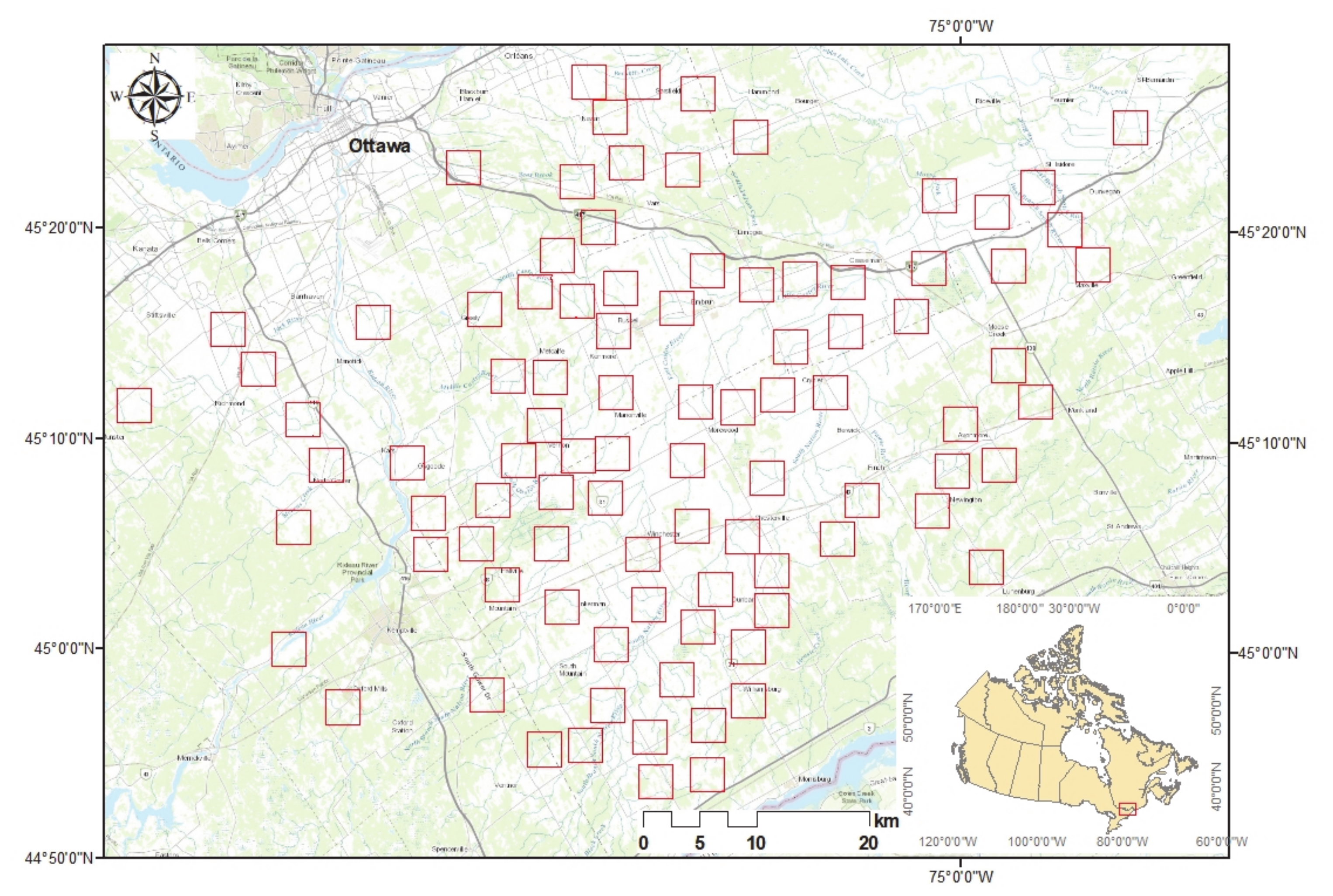
Figure 1. Study area and the geographic location of sample landscapes in Eastern Ontario. The background map is from the ESRI Inc. street basemap.
Remotesensing 12 01479 g001
Figure 2. TS-CMK significant (p ≤ 0.05) positive (green) and negative (red) trends derived from the July average of weekly MODIS NDVI composite data for each year from 2000 to 2011.
Remotesensing 12 01479 g002
Figure 3. Examples of significant positive (green) and negative (red) inter-annual mid-summer MODIS NDVI trends superimposed on Google Earth images of the sample landscapes (yellow squares) taken in 2012.
Remotesensing 12 01479 g003
Figure 4. TS-CMK significant (p ≤ 0.05) positive (green) and negative (red) trends derived from mid-summer Landsat NDVI over the period 1985–2011.
Remotesensing 12 01479 g004
Figure 5. Example of mid-summer Landsat NDVI trend data for one of the sample landscapes showing a temporal break in the trend slope about the year 2000. The sample landscape location is shown on the map on the right.
Remotesensing 12 01479 g005
Figure 6. Percentage of pixels with positive mid-summer Landsat NDVI trends (categorized as five classes) over all sample landscapes during 1985-2000 compared to 2000–2011.
Remotesensing 12 01479 g006
Figure 7. Comparing TS-CMK significant (p ≤ 0.05) positive (green) and negative (red) trends derived from mid-summer Landsat NDVI for 1985–2000 and 2000–2011 in: (a) the entire study area, and (b) several example landscapes delineated within the red rectangles for each period.
Remotesensing 12 01479 g007
Figure 8. Examples of CMK significant negative trends in mid-summer Landsat NDVI for 2000-2011 associated with (a) natural and semi-natural patches (yellow arrows), (b) individual fields (yellow ellipses), and (c) individual field edges (yellow arrows). The background image is from Google Earth, 2012.
Remotesensing 12 01479 g008
Figure 9. Examples of CMK significant positive trends in the mid-summer Landsat NDVI for 2000–2011 associated with agricultural lands (yellow arrows). The background image is from Google Earth, 2012.
Remotesensing 12 01479 g009
Figure 10. Comparing Landsat (top) and MODIS (bottom) spatial patterns of significant negative (red) and positive (green) trends in the mid-summer NDVI. Ellipses with the same colors show the same location on both maps with spatially overlapping significant trends. Arrows show instances of significant positive or negative trends identified by only one dataset.
Remotesensing 12 01479 g010
Figure 11. The relationships between the 2011–2012 plant and beetle gamma diversity and temporal vegetation metrics—plant diversity and the percentage of significant positive trending Landsat NDVI pixels in each sample landscape for 2000–2011 and 1985–2011 (a), plant and beetle diversity and Landsat-derived temporal CV of the mean sample landscape NDVI for 1985–2011 (b), 1985–2000 (c), and 2000–2011 (d).
Remotesensing 12 01479 g011
Table 1. Year and date of the selected Landsat 5 Thematic Mapper (TM) data.
#YearDate#YearDate#YearDate#YearDate
1198513-Jul5199628-Aug9200315-Jul13200812-Jul
2198720 Aug6199730-Jul10200520-Jul14200915-Jul
3199407-Aug7199802-Aug11200607-Jul15201002-Jul
4199510-Aug8200110-Aug12200726-Jul16201105-Jul
Table 2. Number of sample landscapes with 0%–4%, 5%–9%, and more than 10% of pixels showing significant positive or negative trends for MODIS (2000–2011) and Landsat (1985–2011) mid-summer NDVI time series.
Negative TrendPositive Trend
0%–4%5%–9%>10%0%–4%5%–9%>10%
MODIS69186312339
Landsat84900390
Table 3. Cross-tabulation of the number of pixels identified as having significant trends or no trend in MODIS and Landsat mid-summer NDVI time series.
MODIS
NegativePositiveNo trendSum% Agreement
LandsatNegative1190 2300 34,346 37,8363.1
Positive1440 4445 64,402 70,2876.3
No trend16,294 48,537 749,849814,68092.0
Sum18,92455,282848,597922,803
% Agreement6.38.088.4