Development and Testing of a Clear-Sky Data Selection Algorithm for FY-3C/D Microwave Temperature Sounder-2

Abstract

The Fengyun (FY)-3C/D microwave temperature sounder-2 (MWTS-2) is similar to the Advanced Microwave Sounding Unit-A (AMSU-A), except it lacks two window channels located at 23.8 GHz and 31.4 GHz. This makes a clear-sky data determination challenging for the MWTS-2 due to the unavailability of cloud liquid water path (LWP) retrievable from the two window channels. The purpose of this study is to develop a clear-sky data selection algorithm for the FY-3C/D MWTS-2 based on the bias-removed differences between observations and model simulations of the MWTS-2 50.3-GHz channel 1 (or equivalently AMSU-A channel 3). First, a point is defined as a temporal clear-sky (cloudy) point if the bias-removed difference between observed and simulated brightness temperatures is smaller than or equal to (greater than) 2 K. Then, a temporal clear-sky (cloudy) point is defined as a final clear-sky (cloudy) point if all points within its 60-km (100-km) radial distance are temporal clear-sky (cloudy) points. Finally, if the mean value of the bias-removed differences between observations and simulations in the 100-km circle from a temporal cloudy point are smaller than or equal to (greater than) 2 K, all temporal clear-sky points within this circle are (not) taken as the final clear-sky points. Applications of this algorithm to FY-3C MWTS-2 and MetOp-B AMSU-A lead to the following conclusions: (i) more than 70% (95%) of the clear-sky (cloudy) data points are successfully identified from both AMSU-A and MWTS-2 observations; (ii) the algorithm-selected clear-sky data points were located in clear-sky areas in the GOES-15 imager, and (iii) the bias-removed differences between observations and model simulations of MWTS-2 channel 1 well reveals the eye, the eyewall, and the spiral rainband structure of Super Typhoon Halong (2014).

1. Introduction

The China Meteorological Administration (CMA)’s Fengyun (FY)-3 series of satellites are in sun-synchronous polar-orbiting orbits: the environmental research satellites FY-3A/B launched in May 2008 and November 2012, respectively, and the operational platforms FY-3C/D launched in September 2013 and May 2015, respectively [1,2]. The follow-on FY-3E/F/G satellites are scheduled to be put into orbit in 2020, 2021, and 2022, respectively. The FY-3A/B microwave temperature sounders (MWTSs) have four channels with central frequencies similar to the Microwave Sounding Unit (MSU) channels 1–4 and the Advanced MSU-A (AMSU-A) channels 3, 5, 7, and 9 onboard the National Oceanic and Atmospheric Administration (NOAA) series of polar-orbiting satellites [3]. The MWTS-2 instruments onboard the FY-3C/D satellites have a total of 13 oxygen channels with central frequencies ranging from 50.3 GHz to 57.6 GHz [4]. The MWTS-2 plays a critical role in monitoring atmospheric temperatures from the surface to the upper stratosphere, increasing the accuracy of numerical weather prediction (NWP) through MWTS-2 data assimilation and providing observational datasets for global climate change investigations [5]. The MWTS-2 is similar to AMSU-A onboard the NOAA-15/16/17/18/19 satellites and the EUMETSAT MetOp-A/B/C satellites.

In the past 40 years, microwave temperature sounding radiances have been widely assimilated into the NWP models of institutions like the National Centers for Environmental Prediction (NCEP) and the European Centre for Medium-range Weather Forecasts (ECMWF), significantly impacting weather forecast accuracies in a positive way [6,7]. Bias correction (BC), cloud detection, and land surface emissivity are the most challenging problems for microwave radiance assimilation [8]. The errors of the background and observations are assumed to have unbiased Gaussian distributions, where the background is the atmospheric state provided by NWP models. Therefore, the scan-angle-dependent and geographical-dependent bias of cross-track instruments must be carefully quantified and removed before satellite assimilation [9]. It is difficult for radiative transfer models (RTMs) to simulate radiances with cloud effects as accurately as in clear sky conditions due to either a lack of accurate cloud microphysical parameters input or an inconsistency in the use of microphysical parameters between RTMs and NWP models [10]. Clear-sky radiance assimilation has thus been the focus of most investigations [11]. Geer et al. (2012) [12] proposed a symmetrical observation error method based on the liquid water path (LWP) index and observation-minus-background (O-B) departures to assimilate cloudy and rain-affected AMSU-A data. NCEP [13] and the Met Office [14] have also carried out all-weather assimilation experiments. Both clear-sky and all-weather assimilations require cloud information, but the FY-3A/B MWTS and the FY-3C/D/E MWTS-2 do not have the 23.8-GHz and 31.4-GHz channels needed for retrieving cloud LWP [15]. Therefore, the development of a cloud detection scheme for MWTS-2 is critical for assimilating MWTS-2 radiances.

Li and Zou (2013) [16] developed a cloud detection scheme for the FY-3A MWTS by collocating MWTS data with the cloud fraction retrieved by the FY-3A visible and infrared radiometer. The same method was also applied to FY-3C/D MWTS-2 data assimilation in the CMA’s global and regional assimilation and prediction system [17,18]. Similarly, AMSU-A data points were collocated with cloud products from the Moderate Resolution Imaging Spectroradiometer and assimilated into the Weather Research and Forecasting model, leading to a positive effect on typhoon track and intensity forecasts [19]. All the above methods rely on ancillary measurements (VIS/IR). However, the VIS/IR and microwave instruments have different cloud sensitivity and observation resolutions. The error and efficiency of collocations between the two instruments might affect cloud detection results. Niu and Zou (2018; hereafter referred to as N18) [20] found that the O-B values after BC from AMSU-A channel 3 are highly correlated with AMSU-A-retrieved LWP. A cloud detection algorithm without involving another instrument was developed based on some channel-3 O-B related tests, which successfully identified about 50% of AMSU-A clear-sky data points. This study further refines the N18 cloud detection scheme and applies it to MWTS-2 observations with the goal of increasing the success rate of the clear-sky data selection.

This paper is structured as follows. Section 2 briefly introduces the MWTS-2, AMSU-A, and LWP datasets and describes input variables for the community radiative transfer model (CRTM). Section 3 presents the weighting functions (WFs) of MWTS-2 and AMSU-A and the collocations between AMSU-A and MWTS-2 data points. Section 4 describes the latitudinal- and scan-dependent bias estimates for MWTS-2 and AMSU-A channels. In Section 5, a modified clear-sky data selection algorithm is developed. Section 6 illustrates a possible way to monitor Super Typhoon Halong (2014) using AMSU-A and MWTS-2 observations.

2. Data and Model

FY-3C was launched into an orbit with an inclination angle of 98.7° to the equator, whose altitude is about 836 km. MetOp-B also a sun-synchronous satellite and was launched on September 17, 2012. The altitude of MetOp-B is about 827 km which is slightly lower than the altitude of FY-3C. Utilized here are global Level-1B brightness temperatures from the FY-3C MWTS-2 and the MetOp-B AMSU-A, as well as the LWP retrievals derived from AMSU-A channels 1 and 2 [15].

The community radiative transfer model (CRTM 2.3.0) developed by the Joint Center for Satellite Data Assimilation (JCSDA) is used to simulate clear-sky brightness temperatures for AMSU-A and MWTS-2 channels. The uncertainty of surface emissivity obtained from CRTM is large over polar sea ice, snow-covered and desert regions [21], so data over the polar sea ice areas are eliminated from this study. This study only uses the CRTM for clear-sky simulations of brightness temperatures. Compared with the accurate line-by-line radiative transfer model of the monochromatic radiative transfer model (MonoRTM) [22], the precision of the CRTM for clear-sky simulations is better than 0.2 K in the microwave region [23].The input variables for the CRTM are obtained from the ECMWF ERA-5 reanalysis. The ERA-5 reanalysis has a horizontal resolution of 0.25° × 0.25° and 37 vertical pressure levels. To obtain variables at each observed FOV pixel, linear interpolation and Lagrange interpolation are applied to the times and locations, respectively, in the ERA-5 reanalysis [24]. Input variables include the following atmospheric profiles: temperature (unit: K), water vapor mixing ratio (unit: kg kg⁻¹), and ozone (unit: ppmv). The carbon dioxide concentration is set to 390 ppmv. The surface variables are surface type, surface skin temperature (unit: °C), 10-m wind speed (unit: m s⁻¹), and wind direction (unit: degree), and the satellite parameters are the satellite zenith angle and the satellite azimuth angle (unit: degree).

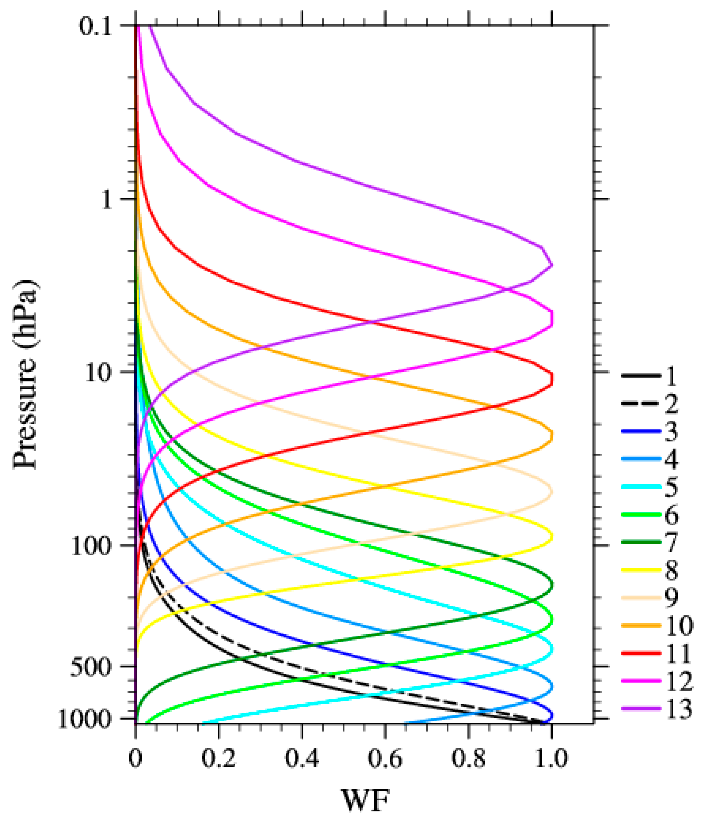
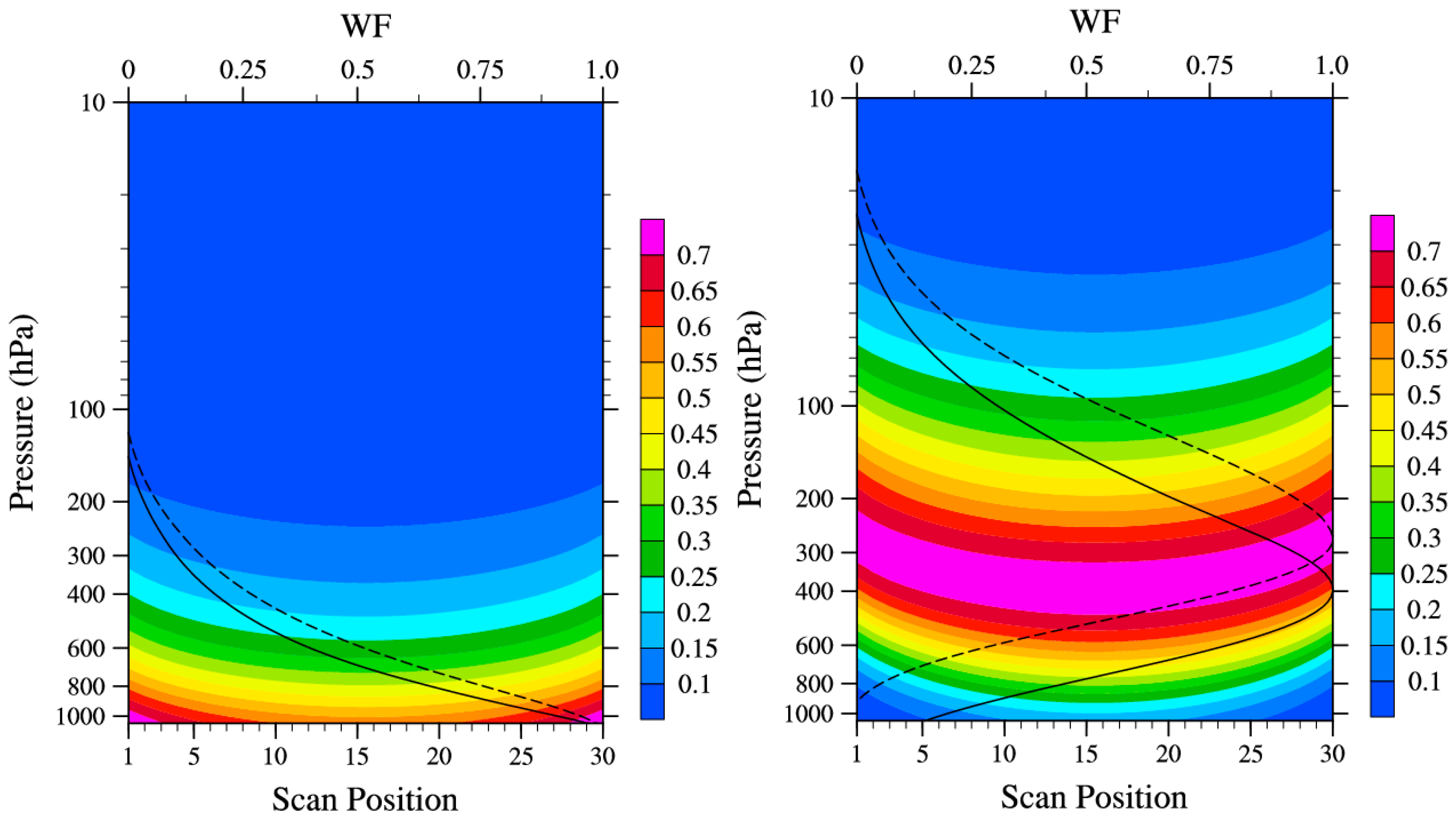
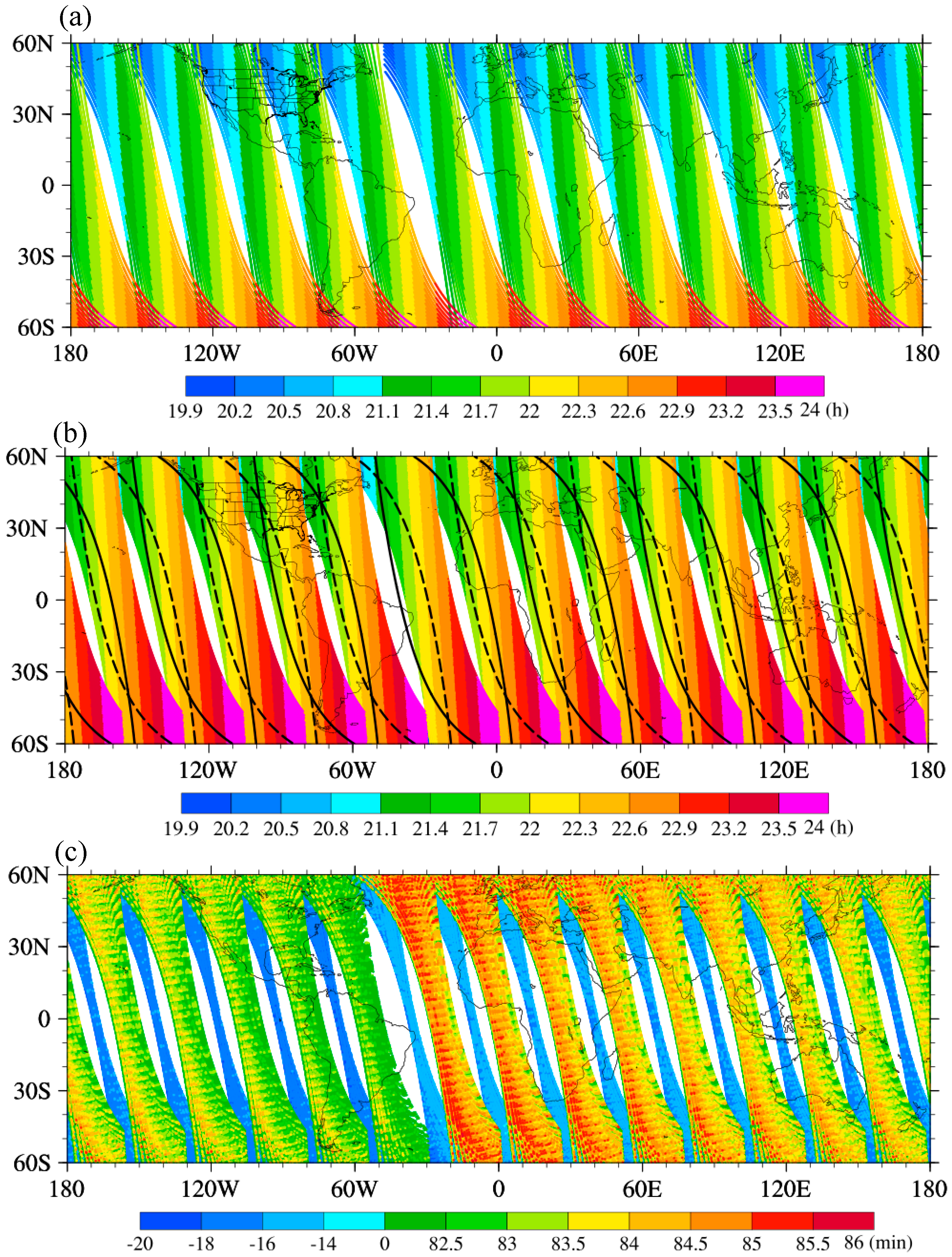
3. Channel Characteristics and Data Collocation

The FY-3C MWTS-2 is a cross-track radiometer. Along a single scanline, it scans 90 fields of view (FOVs) as scan angles vary from −49.5° to +49.5°. The swath width is 2250 km, and the FOV diameter at the nadir is 32 km. The MWTS-2 is similar to the AMSU-A onboard the MetOp-B satellite. AMSU-A is also a cross-track instrument with a scan angle of ±48.5° and a 2300-km swath width. Each AMSU-A scanline has 30 FOVs. The spatial resolution of AMSU-A at the nadir view is 48 km [25].

Table 1. Channel number, frequency, noise equivalent differential temperature (NEDT), bandwidth, polarization, and weighting function peak (WFP) of MetOp-B Advanced Microwave Sounding Unit-A (AMSU-A) and Fengyun (FY)-3C MWTS-2.

Channel No.	Frequency (GHz)		NEDT (K)		Bandwidth (MHz)		WFP (hPa)
AMSU/MWTS	AMSU	MWTS	AMSU	MWTS	AMSU	MWTS
1/-	23.8(V)	-	0.30	-	270	-	1085
2/-	31.4(V)	-	0.30	-	180	-	1085
3/1	50.30(V)	50.30(H)	0.40	1.20	180	180	1085
-/2	-	51.76(H)	-	0.75	-	400	950
4/3	52.80(V)	52.80(H)	0.25	0.75	400	400	850
5/4	53.596(H)		0.25	0.75	170	400	700
6/5	54.400(H)		0.25	0.75	400	400	400
7/6	54.94(V)	54.94(H)	0.25	0.75	400	400	250
8/7	55.500(H)		0.25	0.75	310	330	200
9/8	57.290 (f0) (H)		0.25	0.75	310	330	100
10/9	f0 ±0.217(H)		0.40	1.20	76	78	50
11/10	f0 ±0.322±0.048(H)		0.40	1.20	34	36	25
12/11	f0 ±0.322±0.022(H)		0.60	1.70	15	16	10
13/12	f0 ±0.322±0.010(H)		0.80	2.40	8	8	5
14/13	f0 ±0.322±0.005(H)		1.20	3.60	3	3	2
15/-	89(V)	-	0.05	-	6000	-	1085

presents the channel characteristics of MetOp-B AMSU-A and FY-3C MWTS-2. Considering the instrument channel settings of MWTS-2 and AMSU-A, MWTS-2 does not have the 23.8-, 31.4-, and 89-GHz channels, but has one more 51.76-GHz near-surface channel than the AMSU-A. Although MWTS-2 channel 1 and AMSU-A channel 3 have central frequencies of 50.3 GHz, they have vertical (V) and horizontal (H) polarizations, respectively. The noise equivalent differential temperature (NEDT) of MWTS-2 channel 1 is 1.2 K, which is larger than that of AMSU-A channel 3 (0.4 K). Moreover, the NEDTs of the corresponding MWTS-2 channels are larger than those of the AMSU-A NEDTs, indicating that the measurement precision of MetOp-B AMSU-A is better than FY-3C MWTS-2.

The MWTS-2 measures radiations from the surface to the upper stratosphere using 13 channels with their WFs peak at different altitudes, as shown in Figure 1. The WF is the vertical differential of the atmospheric transmittance, defined as

$$W{F}_{{}_{\lambda }}(p)=\frac{d{\tau }_{\lambda }(p)}{d\ln p},$$

(1)

where the subscript λ represents the central frequency of the specific channel, and ${\tau }_{\lambda }(p)$ represents the transmittance of the atmosphere at the level p. The vertical integration of the WFs from the surface to the top of the atmosphere is one [26]:

$${\displaystyle {\int }_{p_s}^0[\frac{d{\tau }_{\lambda }(p)}{d\ln p}]}d\ln p={\tau }_{\lambda }(0)-{\tau }_{\lambda }(p_s)=1,$$

(2)

where the subscript s represents the surface. A WF’s peak level indicates where the channel has received the most radiation emitted by the atmosphere at or near this level. Since the atmospheric optical path varies for different scan angles, the WFs will also vary with different FOVs. Figure 2 shows the angular dependence of the normalized WFs for AMSU-A channels 3 and 6 by the CRTM using the U.S. standard atmosphere profile. The WF peak height is 400 hPa at nadir (FOV 15), which is lower than that at the limb (280 hPa, FOV 30). Therefore, for cross-track scanning instruments, the effect of the scan-angle-dependent bias is not negligible.

The local equatorial crossing times (LECTs) of FY-3C and MetOp-B are 22:15 and 21:30 local time (LT) at ascending nodes, respectively. The difference between the LECTs of the two satellites is small. Figure 3a,b show the global distributions of MetOp-B AMSU-A and FY-3C MWTS-2 local times (LTs) at ascending nodes on 15 July 2014, where LT is calculated using the following formula:

$$L{T}_{(\lambda ,\phi )}=UT{C}_{(\lambda ,\phi )}\pm \left|\lambda \right|/15,$$

(3)

where UTC represents the Coordinated Universal Time, and λ and φ are the longitude and latitude, respectively. When λ > 0, addition is done, and when λ < 0, subtraction is done. The FY-3C MWTS-2 data point is collocated with the nearest MetOp-B AMSU-A data point. The collocation criteria are (a) the spatial distance $\Delta d$ between two points is less than 50 km, and (b) the LT difference is less than 3 h:

$$\{\begin{array}{l}\Delta d_{\min }<50\mathrm{km}\\ \Delta t<1.5\mathrm{h}\end{array},$$

(4)

$$\Delta d=R\cdot {\cos }^{-1}(\sin {\phi }_1\sin {\phi }_2+\cos {\phi }_1\cos {\phi }_2\cos ({\lambda }_2-{\lambda }_1)).$$

(5)

The subscripts “1” and “2” represent the MWTS-2 and AMSU-A data points, respectively, and R is the radius of the earth. Figure 3c shows the LT differences between AMSU-A and MWTS-2 over collocated overlapped swaths from ascending nodes on 15 July 2014. LT differences of the collocated data points on overlapped swaths are all within 86 min, meaning that the AMSU-A-retrieved LWPs can also be used as reference values for the MWTS-2 data points when evaluating the results obtained by the proposed clear-sky data selection algorithm.

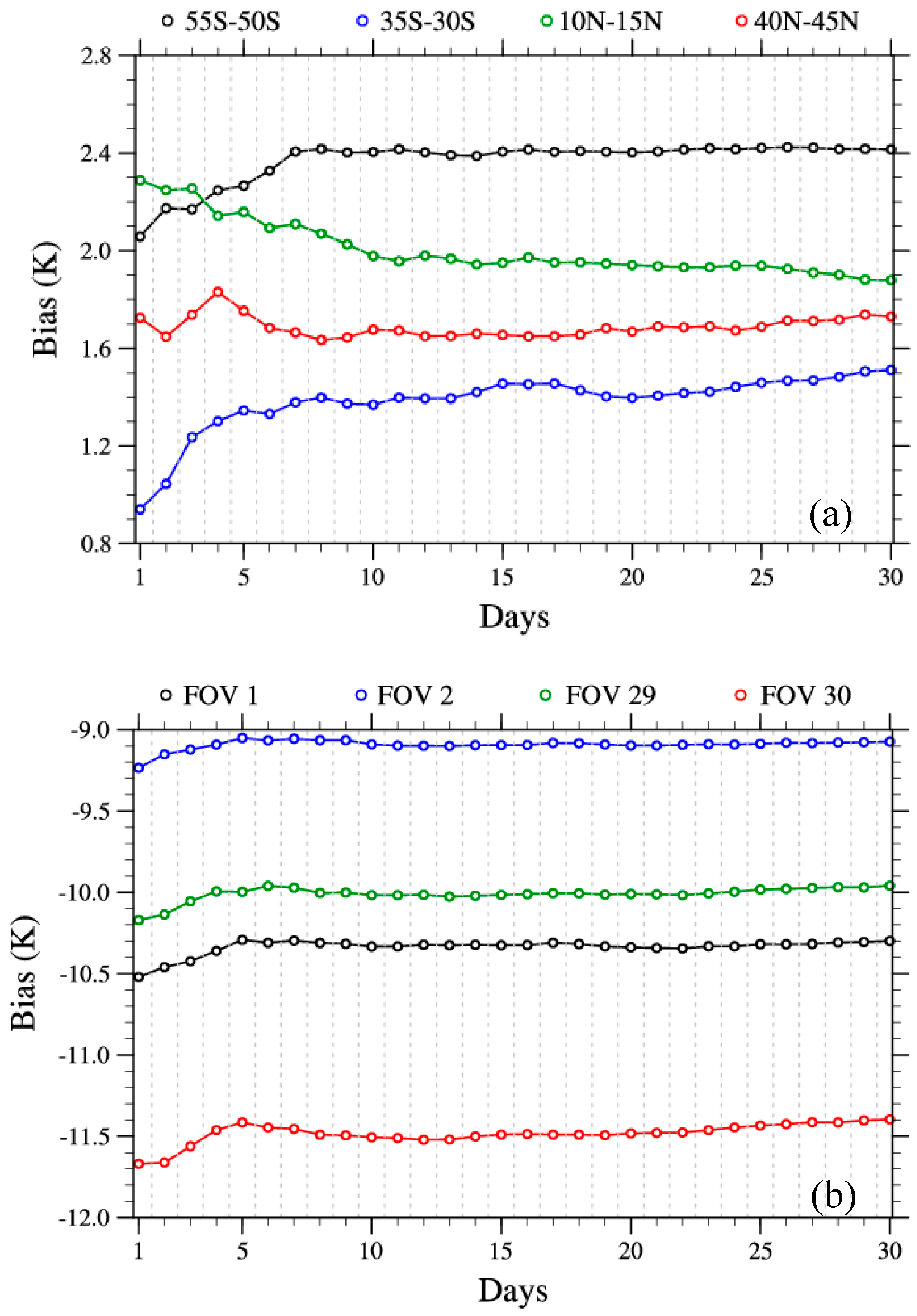
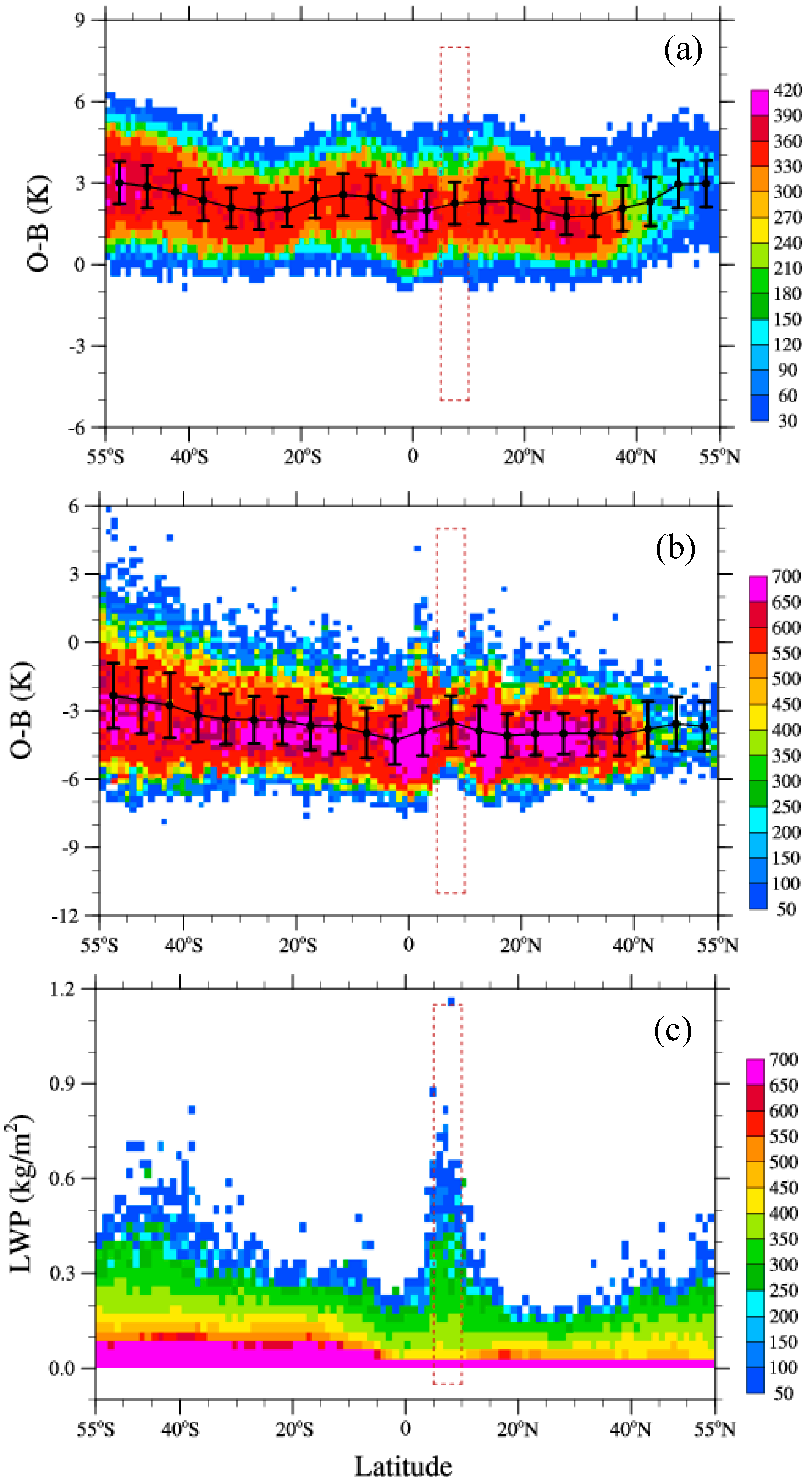
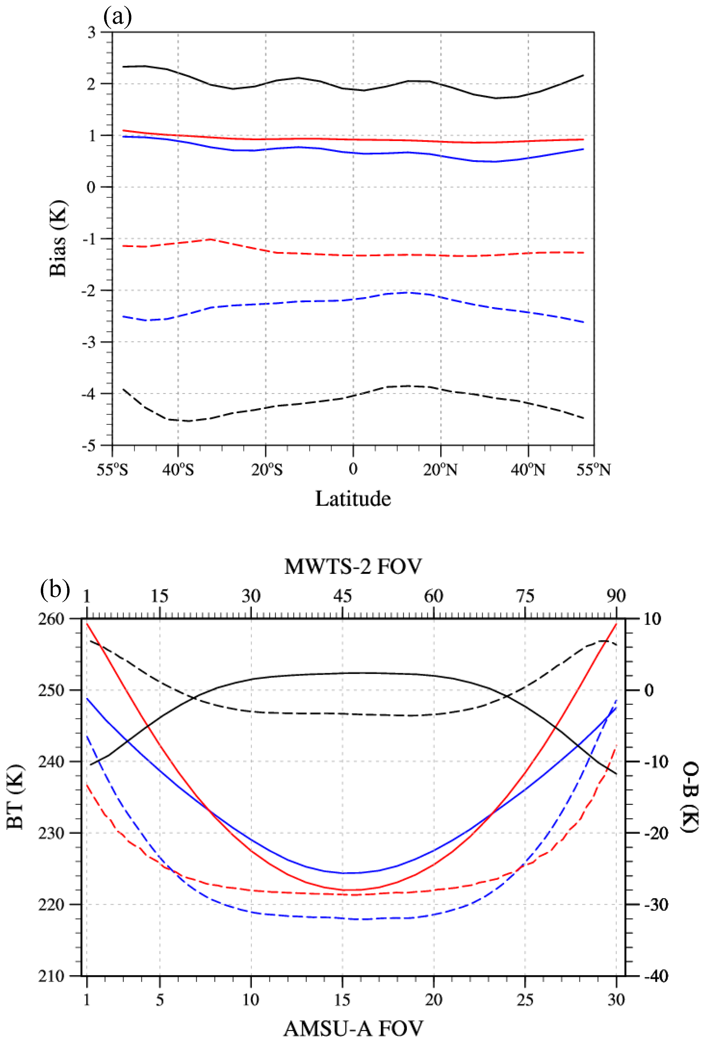
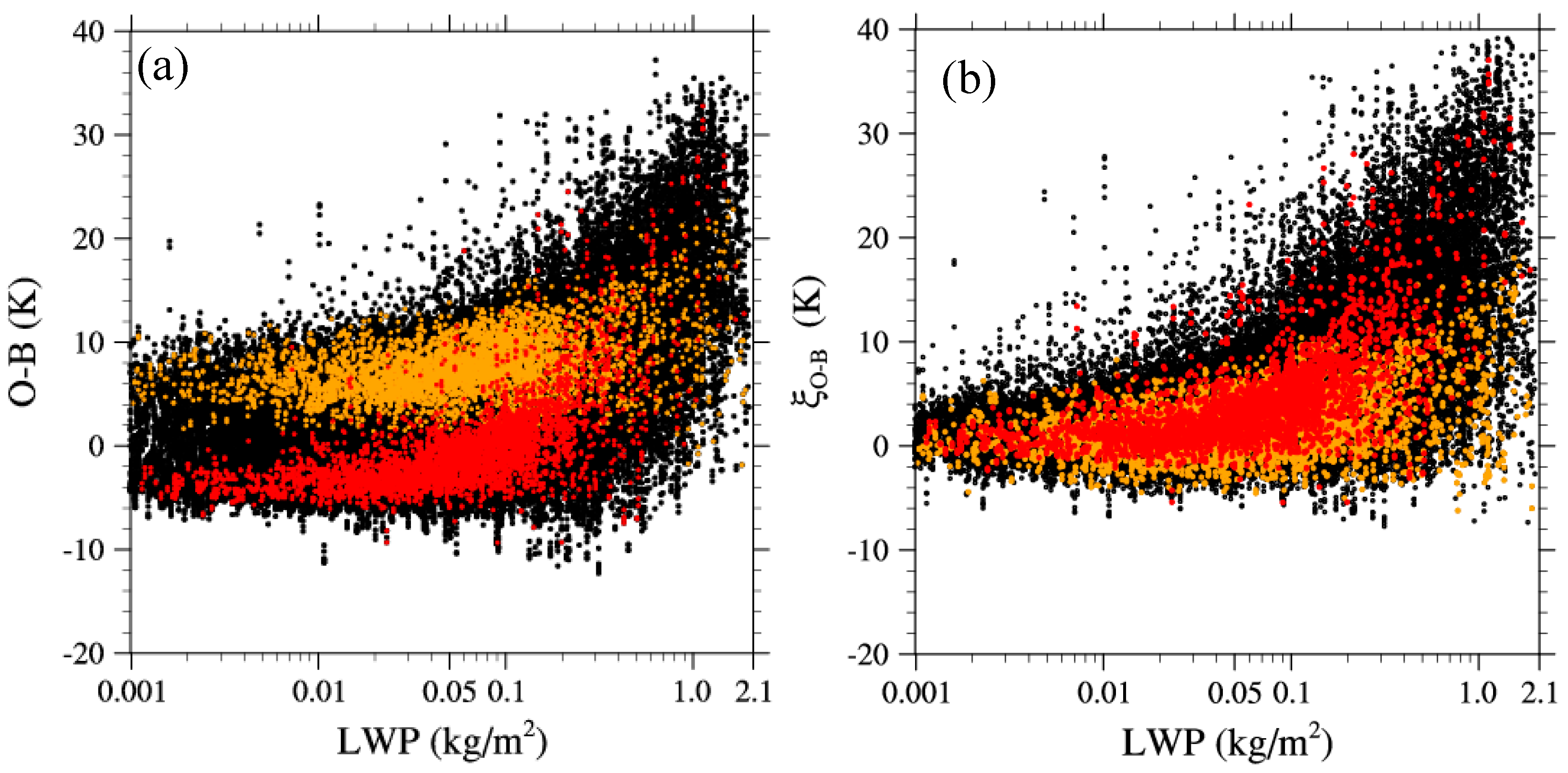
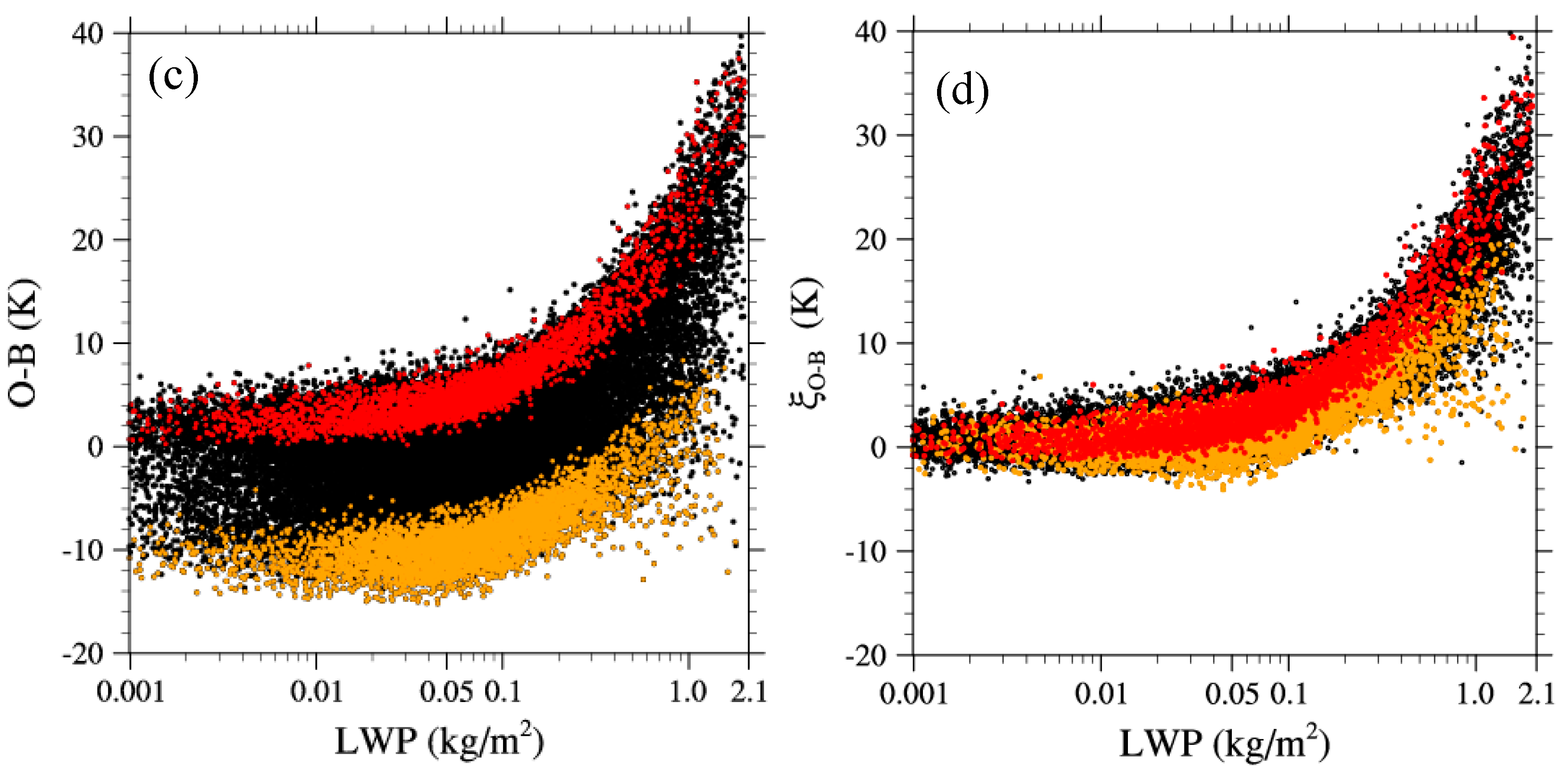
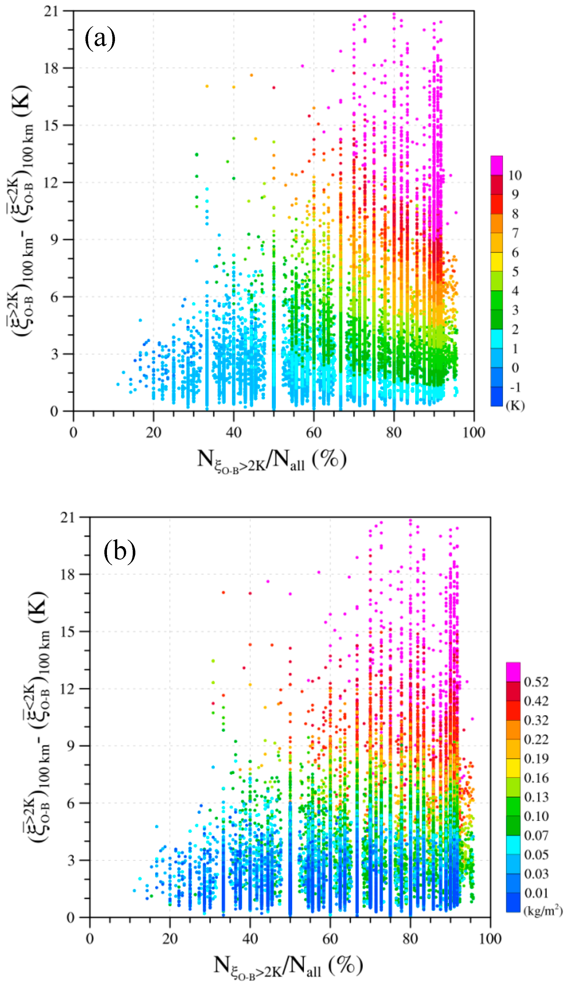
4. Bias Correction of O-B

In this study, a simple BC scheme [27] is used to estimate the scan-angle-dependent bias μ(α) and latitudinal-dependent global mean bias μ(φ) by calculating the moving average differences between observations (O) and clear-sky model simulations (B) calculated by the CRTM with the ERA5 reanalysis data as its input for the previous two weeks of clear-sky oceanic data points. A clear-sky data point is defined as LWP ≤ 0.05 kg m⁻² in this study. In addition, to eliminate the influence of polar sea ice, only data points within 55°S to 55°N are used in this study. We define the following two biases:

$$\mu ({\phi }_i)={\overline{(O-B)}}_{i,nadir},$$

(6)

$$\mu ({\alpha }_j)={\overline{{(O-B)}_j-(O-B)}}_{nadir}.$$

(7)

The subscript “i” stands for the ith 5°-latitudinal band. Only nadir, clear-sky oceanic data points are used to estimate μ(φ). The subscript “j” represents different FOVs along each scanline. The nadir points are FOVs 15 and 16 for AMSU-A and FOVs 45 and 46 for MWTS-2. Figure 4a shows variations in clear-sky O-B biases over the oceans for AMSU-A channel 3 using only nadir data points within different latitudinal bands with respect to the number of days from 1 July to 30 July 2014. The latitudinal-dependent bias is relatively unstable at the beginning when the nadir clear-sky data sample number is small, then stabilizes after two weeks. Similarly, Figure 4b shows variations in the scan-angle-dependent bias at FOVs 1, 2, 29, and 30 for AMSU-A channel 3 with respect to the number of days from 1 July to 30 July 2014. The scan-angle-dependent bias stabilizes by the fifth day. In this study, oceanic clear-sky data points from 1 July to 14 July 2014 are used to estimate latitudinal- and scan-angle-dependent O-B biases, which are then used for obtaining the bias-corrected O-B difference ${\xi }_{O-B}$.

In order to show latitudinal dependences of O-B biases more clearly, we examine the data count distributions of clear-sky oceanic O-B at nadir for both AMSU-A channel 3 as shown in Figure 5a, and the collocated FY-3C MWTS-2 channel 1 as shown in Figure 5b, as well as the AMSU-A LWP shown in Figure 5c from 55°S to 55°N. The means and one-standard deviations are also shown, indicating that O-B biases vary with latitude. The number of nadir clear-sky data points between 40°N and 55°N is small because land areas are larger than ocean areas. The brown dashed box shows the intertropical convergence zone (ITCZ) around 5°N to 10°N in July. There are more cloud systems in the ITCZ, reflected by relatively large LWPs, leading to a small number of clear-sky data points identified by AMSU-A and MWTS-2.

Biases for channels with the same center frequencies could be different for different satellite instruments. This is the case for both the latitudinal shown in Figure 6a and scan-angle shown in Figure 6b dependencies of clear-sky O-B biases for AMSU-A channels 3, 4, and 5 and the similar MWTS-2 channels 1, 3, and 4. Surface-sensitive AMSU-A channel 3 and MWTS-2 channel 1 have larger latitudinal-dependent O-B biases (absolute values), and the other upper channels have smaller latitudinal-dependent O-B bias departures. Larger O-B biases are found at larger scan angles. This is expected for the following reasons: (i) the larger inhomogeneity for limb FOVs with longer optical path lengths, and (ii) surface emissivity ${\epsilon }_s$ is a combination of vertical emissivity ${\epsilon }_V$ and horizontal emissivity ${\epsilon }_H$:

$${\epsilon }_s={\epsilon }_V(\theta ){\cos }^2\theta +{\epsilon }_H(\theta ){\sin }^2\theta ,$$

(8)

where $\theta$ stands for the zenith angles. At the limb, the ratio of ${\epsilon }_H$ over ${\epsilon }_V$ deviates more from unity. Both the AMSU-A and MWTS-2 only observe one polarization. Therefore, polarization approximation errors are larger at the limb.

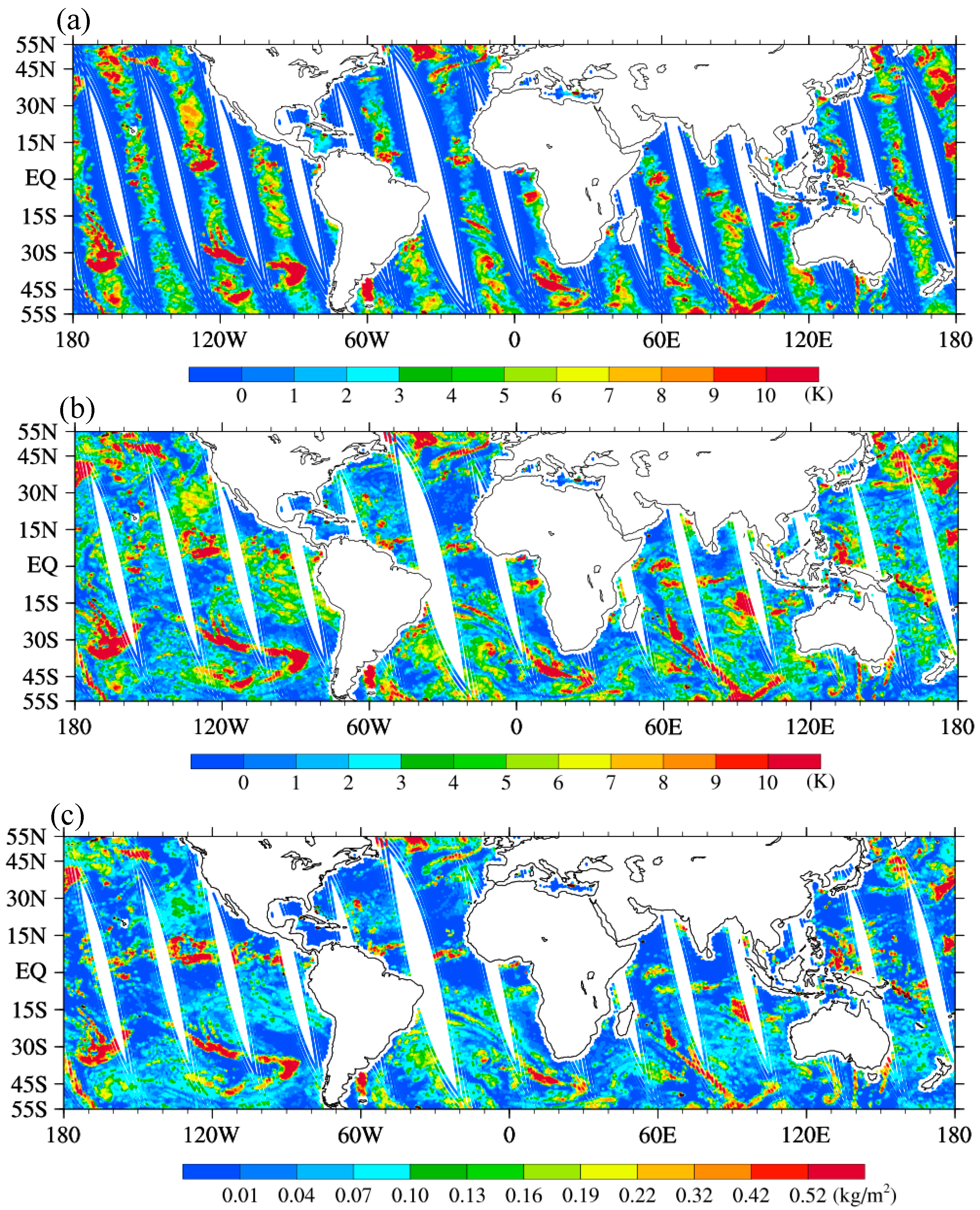
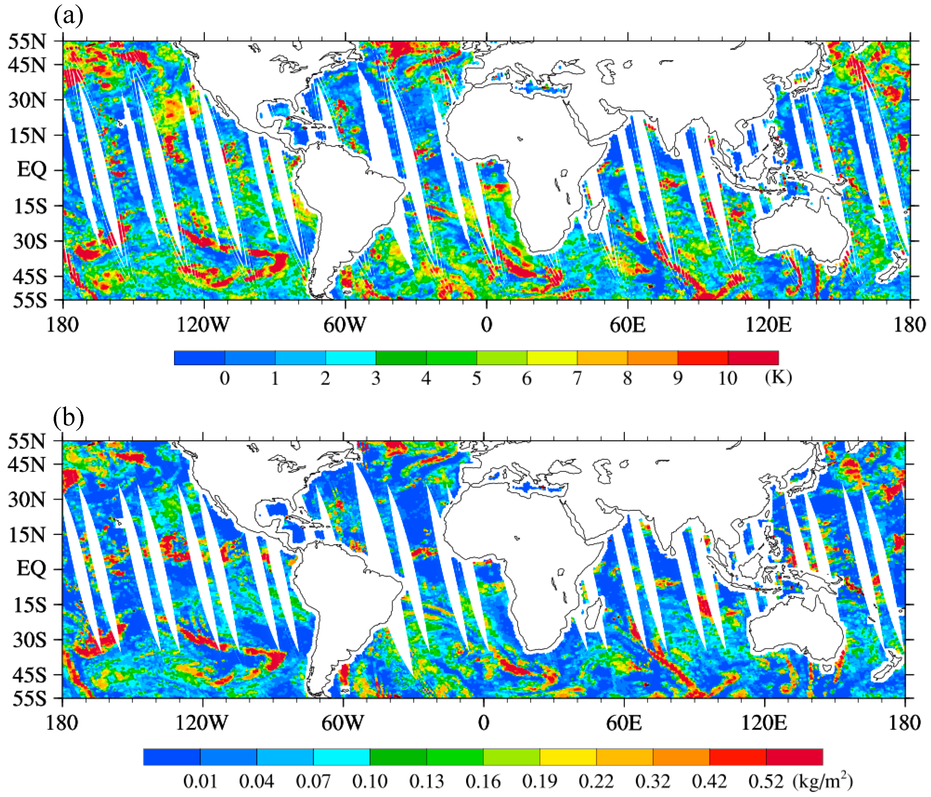
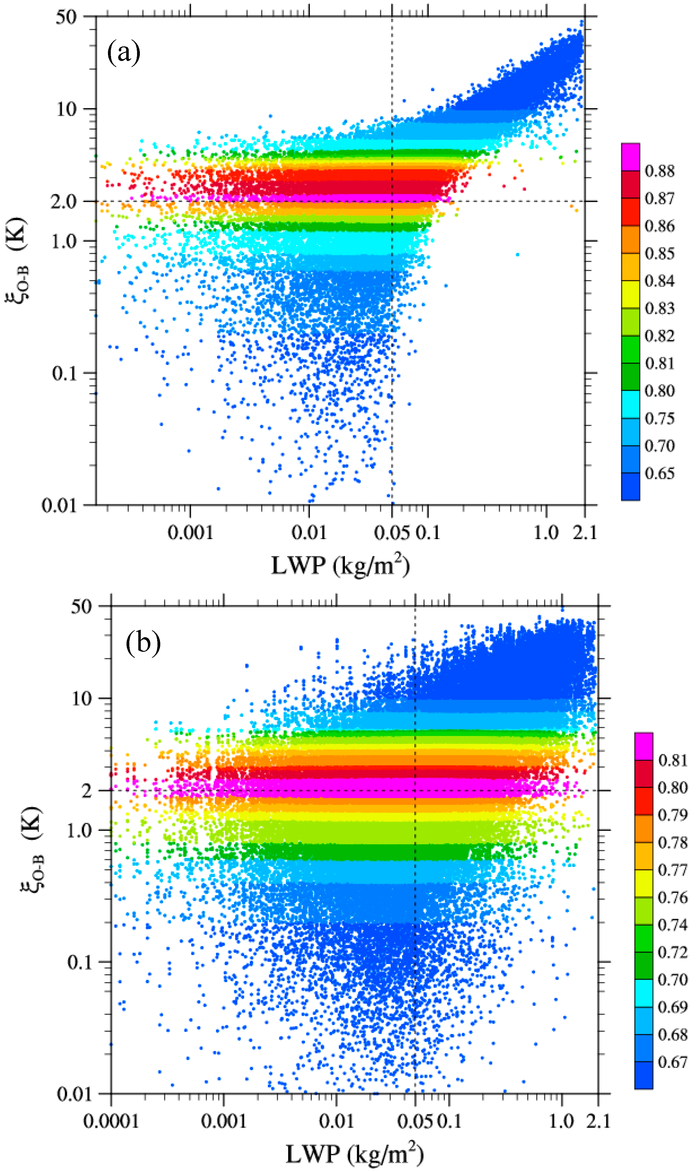
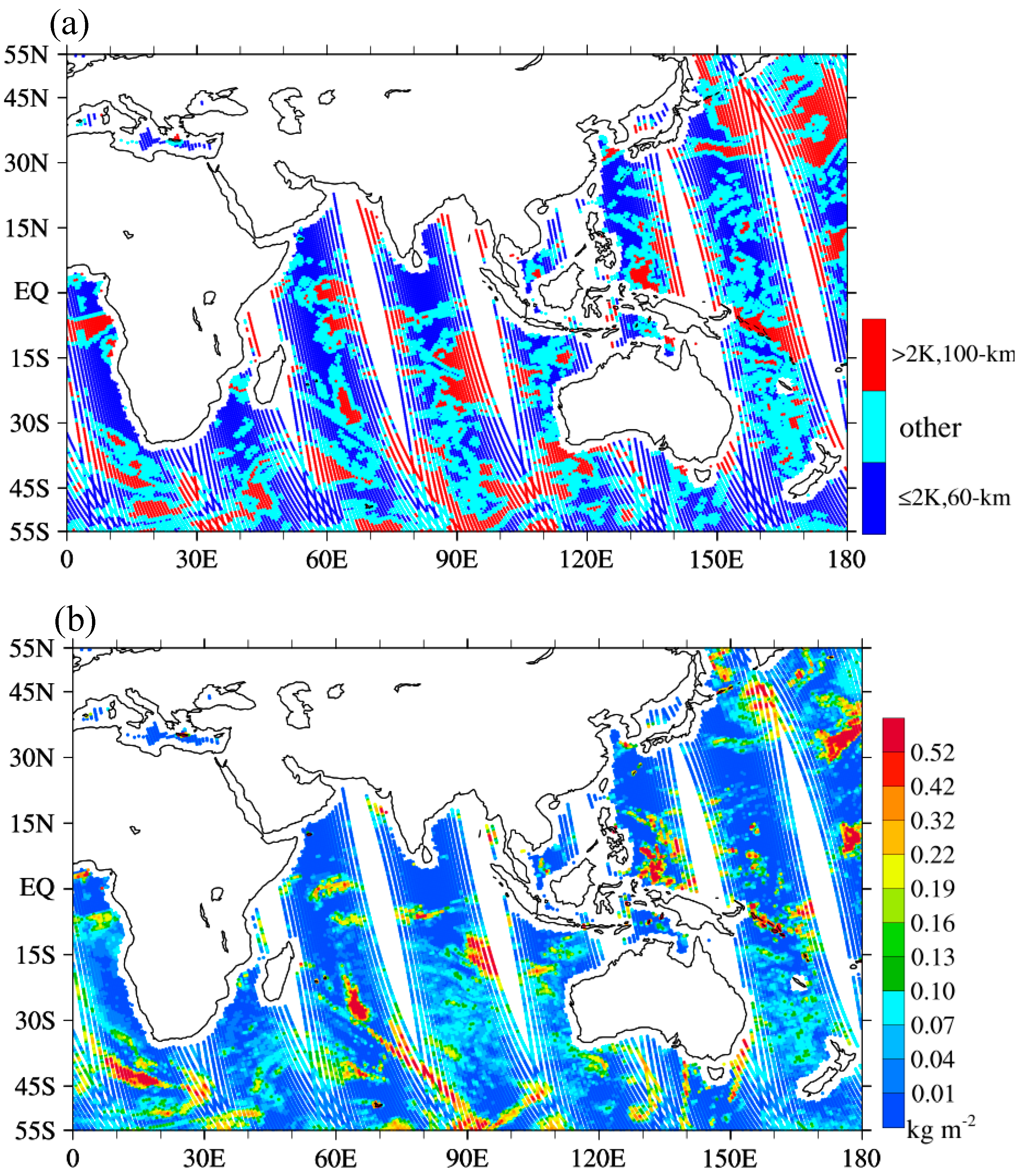
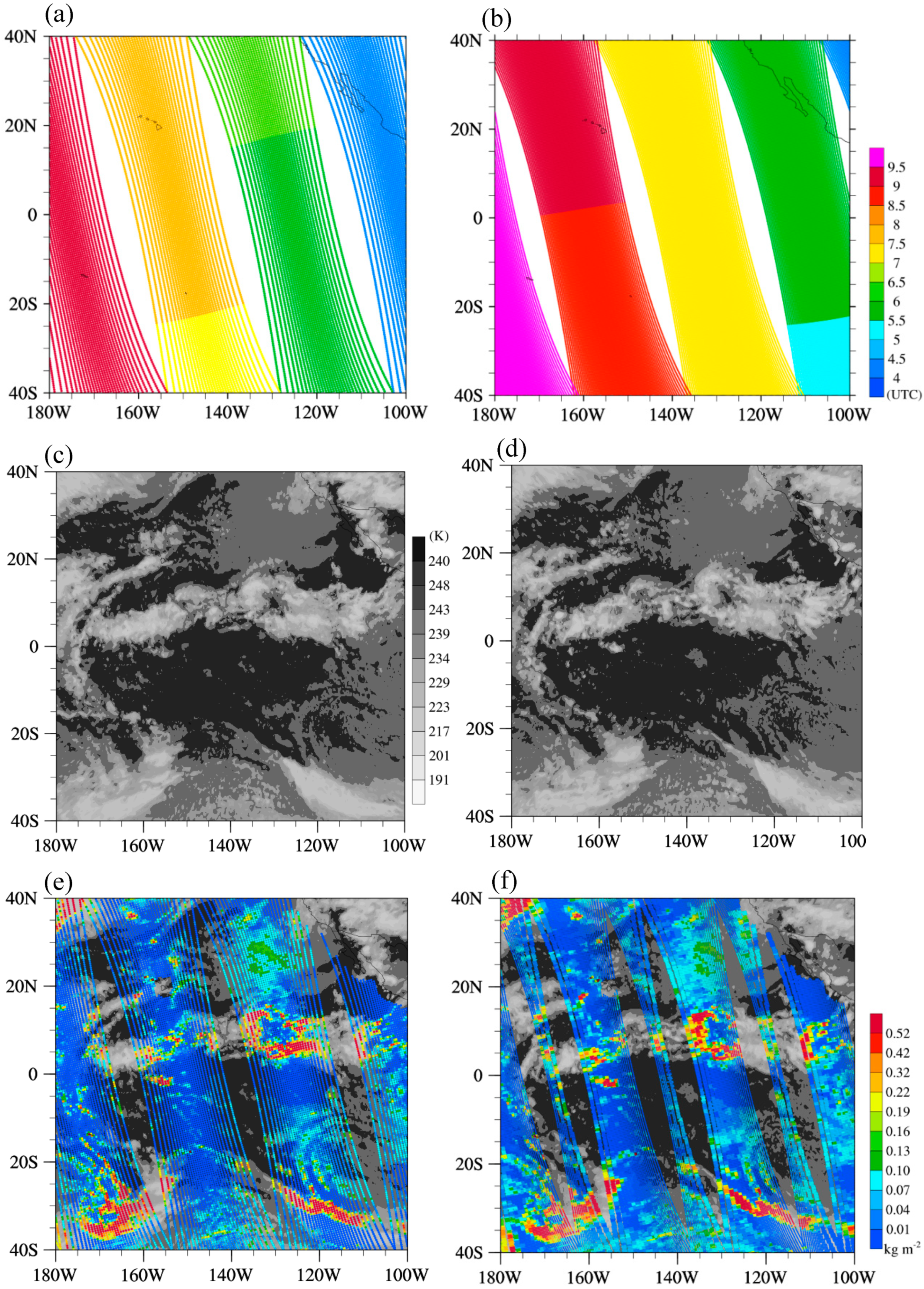
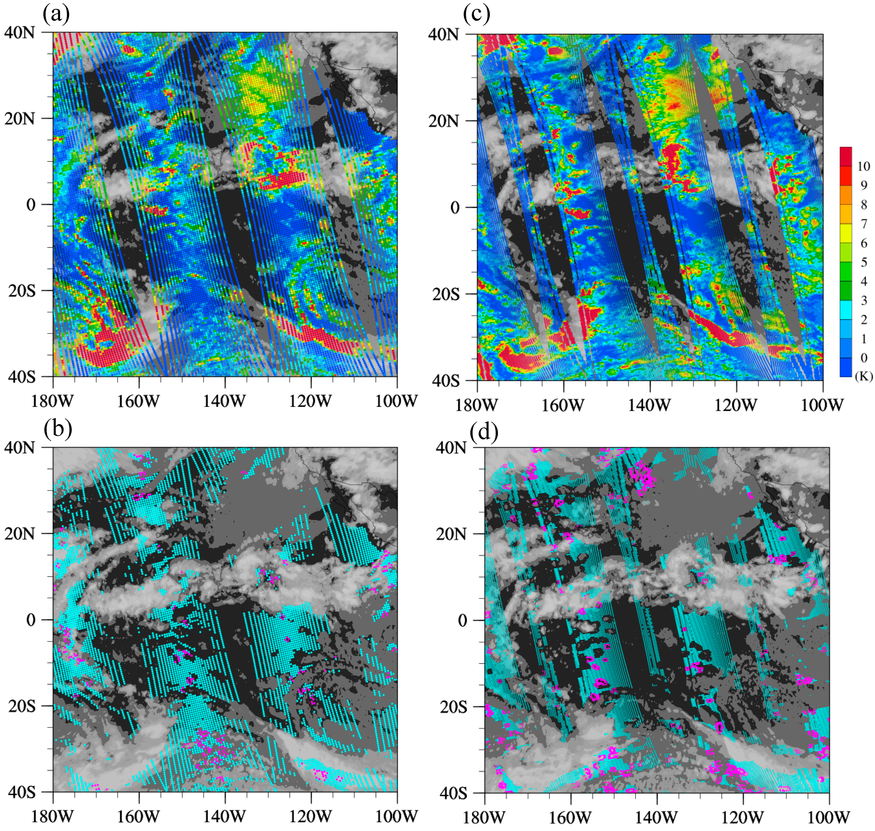
5. Cloud Detection Scheme

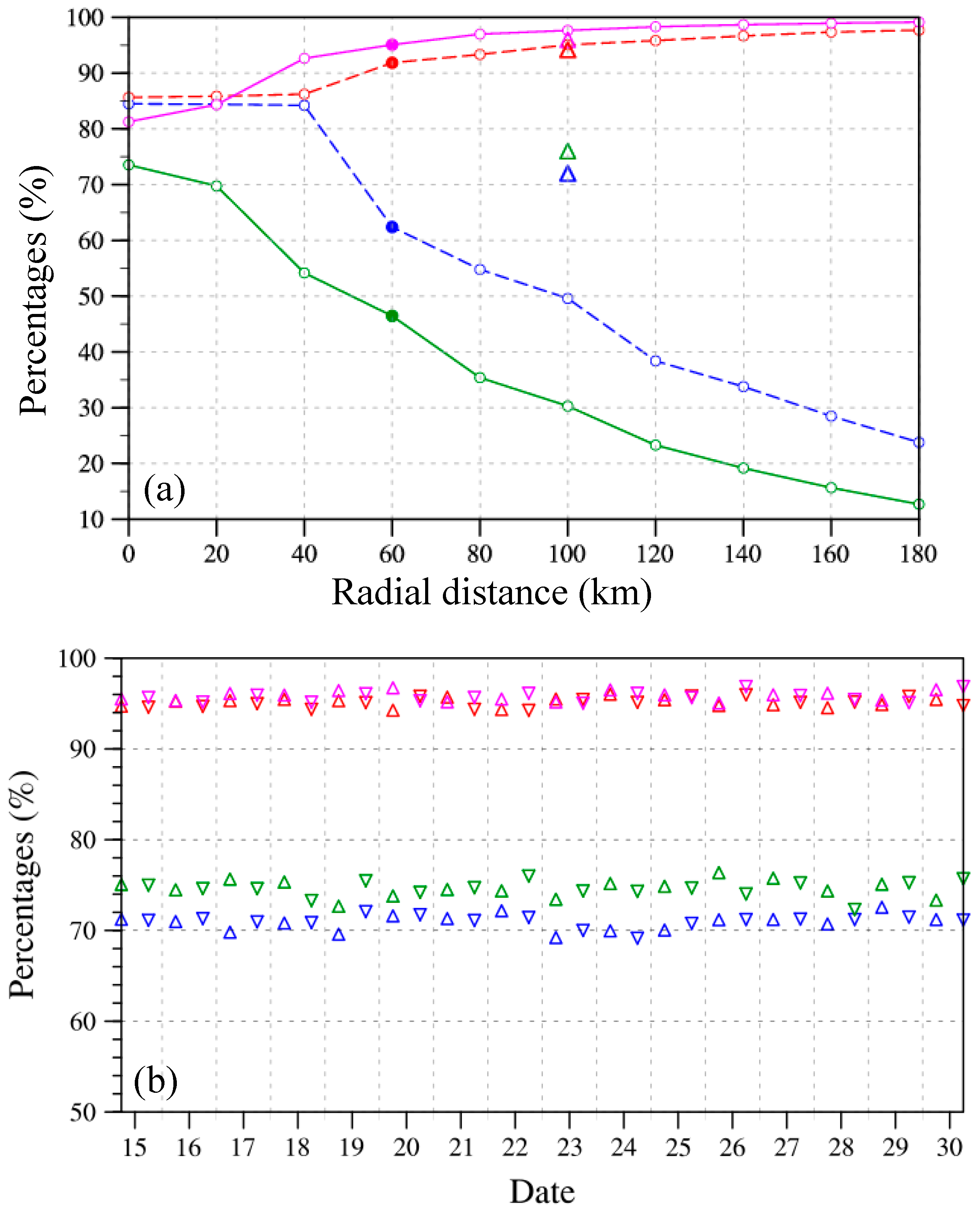
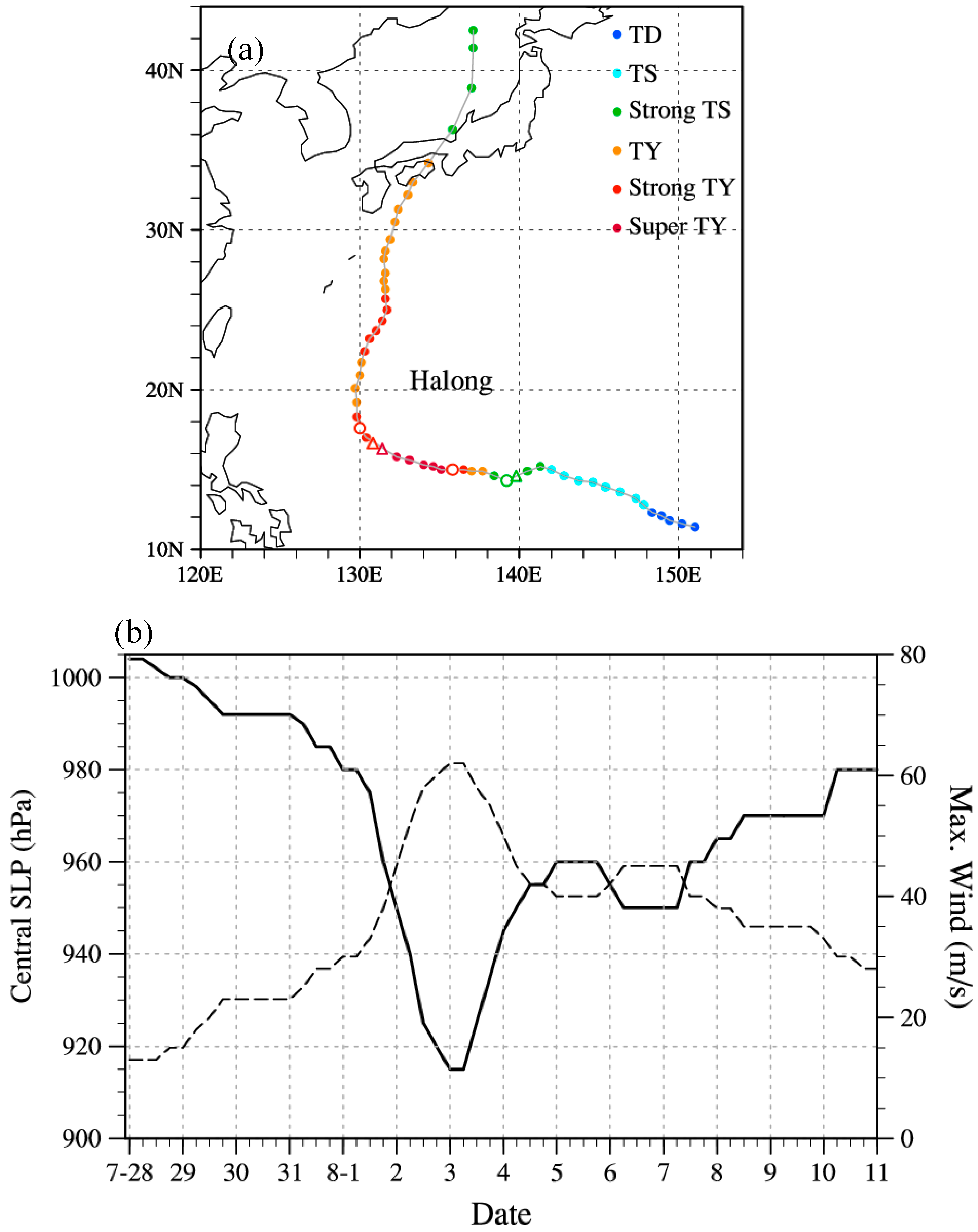
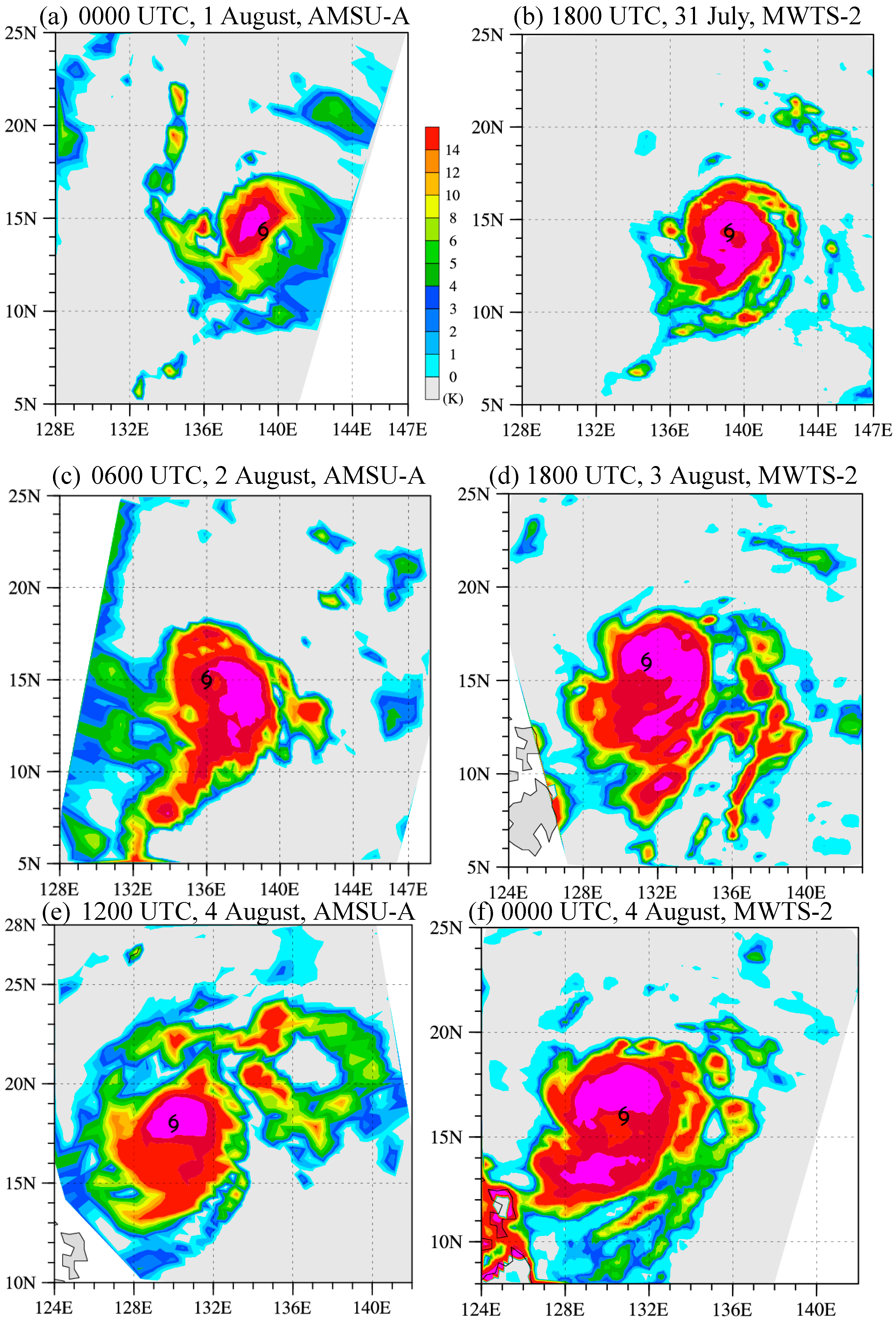
The MWTS-2 is a cross-track microwave radiometer. Therefore, the global features of the differences between observations and model simulations are dominated by a major scan dependence (O-B in Figure 7a), much lower values at large scan angles than at nadir. If we removed the biases μ(φ) and μ(α) from the differences between observations and model simulations, whose global distribution (${\xi }_{O-B}$ in Figure 7b), reveals many of the features in the LWP field, as shown in Figure 7c. As the retrieved LWP is not accurate near coastlines with possibly mixed FOVs, all data points within 50 km of the coastline are not considered in this study. The ${\xi }_{O-B}$ of AMSU-A channel 3 can thus be used for cloud detection. Figure 8 shows the spatial distributions of ${\xi }_{O-B}$ for MWTS-2 channel 1 and the LWP distributions over areas of overlapped orbits between MWTS-2 and AMSU-A at ascending nodes on 15 July 2014. The ${\xi }_{O-B}$ fields of the two channels are well correlated, with a correlation coefficient of ~0.70. Even though the time difference between the two instruments is less than 1.5 h, the movements of deep convective clouds and rapidly evolving cloud systems, especially optically thin clouds, could still cause large differences in local areas. Figure 9 shows scatterplots of O-B and ${\xi }_{O-B}$ for collocated FY-3C MWTS-2 channel 1 and MetOp-B AMSU-A channel 3 versus LWP over oceans at ascending nodes on 15 July 2014. The O-B distributions with FOVs at the limb (orange points) and the nadir (red points) as a function of LWP deviate from each other (left panels). After the BC, all data are evenly distributed (right panels), and the scan-angle-dependent bias is mostly removed. However, the spread of the data points in Figure 9b is larger than that in Figure 9d. This could arise for the reason that the NEDT of MWTS-2 channel 1 is 1.2 K, which is much larger than that of AMSU-A channel 3 (0.4 K).

In this study, first determined is a threshold of ${\xi }_{O-B}$ for AMSU-A channel 3 or FY-3C MWTS-2 channel 1 to identify cloudy or clear-sky data points instead of using LWP. The maximum value of the probability of correct typing (PCT) determines the threshold as follows [28]:

$$PCT=\frac{N(T_{cld}\cap C_{cld}+T_{clr}\cap C_{clr})}{N(T_{cld}+T_{clr})},$$

(9)

where $T_{cld}$ and $T_{clr}$ represent the values of LWP over areas with LWP > 0.05 kg m⁻² and LWP ≤ 0.05 kg m⁻², respectively, and $C_{cld}$ and $C_{clr}$ represent the values of ${\xi }_{O-B}$ over areas with ${\xi }_{O-B}>s$ and ${\xi }_{O-B}\le s$, respectively, where s varies from 0 to 10 K at the 0.2-K interval. Figure 10 shows log–log scatterplots of ${\xi }_{O-B}$ versus LWP for MetOp-B AMSU-A channel 3 and FY-3C MWTS-2 channel 1 on 15 July 2014, showing PCT values at different thresholds for ${\xi }_{O-B}\le s$. The maximum PCT value of 0.88 (0.81) is achieved when ${\xi }_{O-B}=2\mathrm{K}$ for MetOp-B AMSU-A channel 3 (FY-3C MWTS-2 channel 1). When ${\xi }_{O-B}\le 2\mathrm{K}$, both AMSU-A and MWTS-2 may still have cloudy data points (LWP > 0.05 kg m⁻²). In general, these cloudy data points are near the cloud edges. If the N18 scheme is used, all data within a 100-km radial distance of a “cloudy point” (${\xi }_{O-B}>2\mathrm{K}$) are removed, and only 49.5% of clear-sky data points are retained. Further improvements are needed to increase the percentage of correctly detected clear-sky data points.

Having determined the threshold of 2 K in the first step of the proposal algorithm, we take those clear-sky data points for which all data points in its 60-km radial distance satisfy ${\xi }_{O-B}\le 2\mathrm{K}$ as the final clear-sky points in blue, shown in Figure 11a; and those cloudy data points for which all data points in its 100-km radial distance satisfy ${\xi }_{O-B}>2\mathrm{K}$ as the final cloudy points in red, shown in Figure 11a. We denote all other data points as ${\Omega }_1^{remain}$ in cyan, shown in Figure 11a. In the second step of the algorithm, we further determine if the remaining clear-sky data points satisfying ${\xi }_{O-B}\le 2\mathrm{K}$ will be taken as the final clear-sky points. Compared with LWP in Figure 11b, most data points in ${\Omega }_1^{remain}$ are located between the cloudy and clear-sky areas. Figure 12 shows scatterplots of ${({\overline{\xi }}_{O-B}^{>2K})}_{100km}-{({\overline{\xi }}_{O-B}^{\le 2K})}_{100km}$ versus the fraction of “cloudy” data points $\frac{N_{{\xi }_{O-B}>2K}}{N_{all}}$ (N stands for the number of data points) within a 100-km radial distance, showing the mean values of ${\overline{\xi }}_{O-B}$ within the relevant 100-km radial distance in Figure 12a and the mean LWP in Figure 12b. Only ${\Omega }_1^{remain}$ from 15 July to 18 July 2014 are included. The corresponding average LWP is mostly greater than 0.05 kg m⁻² when ${\overline{\xi }}_{O-B}>2\mathrm{K}$, indicating that the average state within 100-km is cloudy. When ${\overline{\xi }}_{O-B}\le 2\mathrm{K}$, the corresponding average LWP is mostly less than 0.05 kg m⁻², suggesting that apart from “cloudy” data points, most of the surrounding data points are clear-sky. Therefore, all data within a 100-km radial distance of a “cloudy point” satisfying ${\xi }_{O-B}\le 2\mathrm{K}$ are removed only if ${\overline{\xi }}_{O-B}>2\mathrm{K}$.

We may make a comparison of the spatial distribution of AMSU-A LWP at the AMSU-A and MWTS-2 swaths with the GOES-15 cloud imagers. Figure 13a,b show MetOp-B AMSU-A and FY-3C MWTS-2 data times in UTC, respectively, and Figure 13c,d show GOES-15 10.7 μm imagery brightness temperature observations at 0600 UTC and 0900 UTC on 15 July 2014, respectively. Also shown are the AMSU-A LWP in Figure 13e and the collocated MWTS-2 LWP in Figure 13f. Data points with large LWP are generally located in cloudy areas seen in the GOES-15 imagery. Figure 14 shows the spatial distribution of ${\xi }_{O-B}$ for MetOp-B AMSU-A channel 3 in Figure 14a and MWTS-2 channel 1 in Figure 14c, which can well reflect the distribution and structure of cloudy regions. Figure 14b,d are the clear-sky data points finally retained by AMSU-A and MWTS-2. Cyan points are the clear-sky data points retained in step 1, and magenta points are additional clear-sky data points found by step 2. These clear-sky points are generally located in clear areas seen in the GOES-15 imagery, indicating that the clear-sky selection algorithm works well.

Figure 15a shows variations of the percentages of correctly identified cloudy data and successfully selected clear-sky data with respect to the radial distance from a cloudy point are provided in Figure 15a. In the N18 scheme, all clear-sky data within the 60-km radial distance from a cloudy point satisfying ${\xi }_{O-B}>2\mathrm{K}$ are discarded. Results obtained by the newly proposed scheme are also included. In the N18 scheme, when the radial distance is set at 100 km, the percentage of correctly rejected cloudy data reaches above 95%, but the percentage of identified clear-sky data is below 50%. When the radial distance is reduced to 60 km, the percentage of identified cloudy data decreases. Using the newly proposed scheme, the percentage of correctly selected clear-sky (cloudy) data points are above 70% (95%) based on AMSU-A and MWTS-2 observations. Figure 15b shows daily variations in the percentages of correctly selected clear-sky and successfully rejected cloudy data from AMSU-A and MWTS-2 at both ascending and descending nodes during 15–30 July 2014. Results are consistent during this half-month period. The percentages of correctly selected clear-sky MWTS-2 data points are slightly higher than those of AMSU-A through this period.

6. Typhoon Halong

As a by-product, the bias-removed differences between observations of model simulations of MWTS-2 channel 1 and AMSU-A channel 3 can be used for monitoring tropical cyclones. We selected typhoon Halong as a case study. Halong was a Pacific typhoon that originated at sea near Chuuk (149.5°E, 7.5°N) on 29 July 2014, pounding the coast of Shikoku, Japan, on 10 August 2014. The best-track tropical cyclone data used for Halong are obtained from the China Meteorological Administration (tcdata.typhoon.org.cn) [29], which include latitude and longitude of cyclone center as shown in Figure 16a, the minimum sea-level pressure (MSLP) and the maximum sustained surface wind speed (MSSW) as shown in Figure 16b at 6-h intervals. The open circles and triangles in Figure 16a indicate the AMSU-A and MWTS-2 observation times, respectively, and are intended to show the potential monitoring abilities of these two instruments for typhoons. During the period 0000 UTC to 0600 UTC 3 August, the MSLP of Halong reached 915 hPa, and the sustained surface maximum wind speed was 61 m s⁻¹, intensifying Halong to a Category-5 typhoon. Figure 17 shows the spatial distributions of ${\xi }_{O-B}$ for AMSU-A channel 3 around 1 August 0000 UTC, 2 August 0600 UTC, and 4 August 1200 UTC, 2014, as well as the MWTS-2 channel 1 ${\xi }_{O-B}$ at 31 July 1800 UTC, 3 August 1800 UTC, and 4 August 0000 UTC, 2014. Due to the significant time differences between AMSU-A observed in the left panel in Figure 17 and MWTS-2 observed in the right panel in Figure 17, the patterns of their ${\xi }_{O-B}$ are not the same. The quantity ${\xi }_{O-B}$ can reflect the horizontal structures of the typhoon, i.e., the typhoon eye, eyewall, and peripheral spiral rainband. This shows that although these instruments cannot directly monitor typhoons in the same way that imagers can, the ${\xi }_{O-B}$ of MWTS-2 channel 1 (AMSU-A channel 3) can be used for monitoring the track and horizontal structures of typhoons.

7. Discussion and Conclusions

In this paper, a clear-sky data selection algorithm is developed and tested for the MWTS-2 data from the FY-3C satellite. In the first step of the algorithm, based on high correlations between the bias-removed differences between observations and model simulations of MWTS-2 channel 1 and collocated AMSU-A retrieved LWP, we determined a threshold of 2 K for determining clear-sky data points. Data points for which the bias-removed differences between observations and model simulations of MWTS-2 channel 1 are smaller or equal to (greater than) 2 K and are defined as temporal clear-sky (cloudy) points. In the second step, a temporal clear-sky (cloudy) point is defined as a final clear-sky (cloudy) point if all points within its 60-km (100-km) radial distance are temporal clear-sky (cloudy) points. In the third step, if the mean bias-corrected O-B differences within the 100-km radial distance of a cloudy point (satisfying bias-corrected O-B differences greater than 2 K) is greater than (less than or than equal to) 2 K, which means that the cloudy (clear-sky) points dominate in the 100-km neighborhood of this cloudy point, the clear-sky points in the neighborhood of this cloudy point will not (will) be selected as the final clear-sky data.

The success rate of the selection of clear-sky data points is more than 75% for the FY-3C MWTS-2. More than 95% of cloudy data points are identified by the FY-3C MWTS-2. This success rate of the clear-sky data selection is 20% higher than that of N18 scheme that removed all data points within a 60-km radial distance from a “cloudy” point. This means that more MWTS-2 clear-sky radiances can be assimilated in a clear-sky data assimilation system. The clear-sky data selection algorithm developed in this study will be incorporated into the MWTS-2 clear-sky data assimilation in the China Meteorological Administration (CMA) Global/Regional Assimilation and Prediction System (GRAPES) 4D-Var operational system [30]. It will also be used for an investigation assessing the uncertainty of AMSU-A/MWTS-2 derived temperature trends in relation to clouds and precipitation over oceans [31].

The spatial distribution of the bias-removed differences between observations and model simulations of MWTS-2 channel 1 and AMSU-A channel 3 are consistent with the LWP field in terms of cloud structures. Therefore, they can be used to monitor typhoons to capture the typhoon eye, eyewall, and outer spiral rainbands. Applying FY-3C/D MWTS-2 data to typhoon monitoring, enhanced by a warm-core retrieval, will be the focus of future investigations.

References

1. Lu, Q.F.; Lawrence, H.; Bormann, N.; English, S.; Lean, K.; Atkinson, N.; Bell, W.; Carminati, F. An evaluation of FY-3C satellite data quality at ECMWF and the Met Office. ECMWF Tech. Memo. 2015, 767, 35. [Google Scholar]
2. Carminati, F.; Candy, B.; Bell, W.; Atkinson, N. Assessment and assimilation of FY-3 humidity sounders and imager in the UK Met Office global model. Adv. Atmos. Sci. 2018, 35, 942–954. [Google Scholar] [CrossRef]
3. Zou, X.; Weng, F.; Zhang, B.; Lin, L.; Qin, Z.; Tallapragada, V. Impacts of assimilation of ATMS data in HWRF on track and intensity forecasts of 2012 four landfall hurricanes. J. Geophys. Res. Atmos. 2013, 118, 11–558. [Google Scholar] [CrossRef]
4. Tian, X.X.; Zou, X.L.; Yang, S.P. A limb correction method for the Microwave Temperature Sounder 2 and its applications. Adv. Atmos. Sci. 2018, 35, 1547–1552. [Google Scholar] [CrossRef]
5. Zou, X.; Wang, X.; Weng, F.; Li, G. Assessments of Chinese FengYun microwave temperature sounder (MWTS) measurements for weather and climate applications. J. Atmos. Oceanic Technol. 2011, 28, 1206–1227. [Google Scholar] [CrossRef]
6. McNally, A.P.; Derber, J.C.; Wu, W.; Katz, B.B. The use of TOVS Level-1B radiances in the NCEP SSI analysis system. Quart. J. Roy. Meteor. Soc. 2000, 126, 689–724. [Google Scholar] [CrossRef]
7. Li, J.; Zou, X. Impact of FY-3A MWTS radiances on prediction in GRAPES with comparison of two quality control schemes. Front. Earth Sci. 2014, PRC 8, 251–263. [Google Scholar] [CrossRef]
8. Dee, D.P. Bias and data assimilation. Quart. J. Roy. Meteor. Soc. 2005, 131, 3323–3343. [Google Scholar] [CrossRef] [Green Version]
9. Auligné, T.; McNally, A.P.; Dee, D.P. Adaptive bias correction for satellite data in a numerical weather prediction system. Quart. J. Roy. Meteor. Soc. 2007, 133, 631–642. [Google Scholar] [CrossRef]
10. Amerault, C.; Zou, X. Comparison of observed and model-simulated microwave radiance in hurricane environment and estimate of background error covariances for hydrometeor variables. Mon. Wea. Rev. 2006, 134, 745–758. [Google Scholar] [CrossRef]
11. Saunders, R.; Hocking, J.; Turner, E.; Rayer, P.; Rundle, D.; Brunel, P.; Vidot, J.; Rocquet, P.; Matricardi, M.; Geer, A.; et al. An update on the RTTOV fast radiative transfer model (currently at version 12). Geosci. Model Dev. 2018, 11, 2717–2737. [Google Scholar] [CrossRef] [Green Version]
12. Geer, A.J.; Bauer, P.; English, S. Assimilating AMSU-A temperature sounding channels in the presence of cloud and precipitation. ECMWF Tech. Memo. 2012, 670, 41. [Google Scholar]
13. Zhu, Y.; Derber, J.; Collard, A.; Dee, D.; Treadon, R.; Gayno, G.; Jung, J.A. Enhanced radiance bias correction in the National Centers for Environmental Prediction’s Gridpoint Statistical Interpolation data assimilation system. Quart. J. Roy. Meteor. Soc. 2014, 140, 1479–1492. [Google Scholar] [CrossRef]
14. Migliorini, S.; Candy, B. All-sky satellite data assimilation of microwave temperature sounding channels at the Met Office. Quart. J. Roy. Meteor. Soc. 2019, 145, 867–883. [Google Scholar] [CrossRef]
15. Grody, N.; Zhao, J.; Ferraro, R.; Weng, F.; Boers, R. Determination of precipitable water and cloud liquid water over oceans from the NOAA-15 advanced microwave sounding unit. J. Geophys. Res. Atmos. 2001, 106, 2943–2953. [Google Scholar] [CrossRef]
16. Li, J.; Zou, X. A quality control procedure for FY-3A MWTS measurements with emphasis on cloud detection using VIRR cloud fraction. J. Atmos. Oceanic Technol. 2013, 30, 1704–1715. [Google Scholar] [CrossRef] [Green Version]
17. Li, J.; Liu, G.Q. Direct assimilation of Chinese FY-3C Microwave Temperature Sounder-2 radiances in the global GRAPES system. Atmos. Meas. Tech. 2016, 9, 3095–3113. [Google Scholar] [CrossRef] [Green Version]
18. Qin, L.; Chen, Y.; Yu, T.; Ma, G.; Guo, Y.; Zhang, P. Dynamic channel selection of microwave temperature sounding channels under cloudy conditions. Remote Sens. 2020, 12, 403. [Google Scholar] [CrossRef] [Green Version]
19. Han, H.; Li, J.; Goldberg, M.; Wang, P.; Li, J.; Li, Z.; Sohn, B.-J.; Li, J. Microwave sounder cloud detection using a collocated high-resolution imager and its impact on radiance assimilation in tropical cyclone forecasts. Mon. Wea. Rev. 2015, 144, 3937–3959. [Google Scholar] [CrossRef]
20. Niu, Z.; Zou, X. Development of a new algorithm to identify clear-sky MSU data using AMSU-A data for verification. IEEE Trans. Geosci. Remote Sens. 2018, 57, 700–708. [Google Scholar] [CrossRef]
21. Liu, Q.; Weng, F. A microwave polarimetric two-stream radiative transfer model. J. Atmos. Sci. 2002, 59, 2396–2402. [Google Scholar] [CrossRef]
22. Clough, S.A.; Shephard, M.W.; Mlawer, E.J.; Delamere, J.S.; Iacono, M.J.; Cady-Pereira, K.; Boukabara, S.; Brown, P.D. Atmospheric radiative transfer modeling: A summary of the AER codes. J. Quant. Spectrosc. Radiat. Transf. 2005, 91, 233–244. [Google Scholar] [CrossRef]
23. Zou, X.; Lin, L.; Weng, F. Absolute calibration of ATMS upper level temperature sounding channels using GPS RO observations. IEEE Trans. Geosci. Remote Sens. 2014, 52, 1397–1406. [Google Scholar] [CrossRef]
24. Li, X.; Zou, X. Bias characterization of CrIS radiance at 399 selected channels with respect to NWP model simulation. Atmos. Res. 2017, 196, 164–181. [Google Scholar] [CrossRef]
25. Wang, X.; Zou, X. An assessment of the FY-3A Microwave Temperature Sounder using the NCEP numerical weather prediction model. IEEE Trans. Geosci. Remote Sens. 2012, 50, 4860–4874. [Google Scholar] [CrossRef]
26. Zou, C.-Z.; Wang, W.; Wang, L.; Long, C. Recalibration and merging of SSU observations for stratospheric temperature trend studies. J. Geophys. Res. Atmos. 2016, 119, 13–180. [Google Scholar] [CrossRef]
27. Li, X.; Zou, X. An alternative bias correction scheme for CrIS data assimilation in regional model. Mon. Weather Rev. 2019, 147, 809–839. [Google Scholar] [CrossRef]
28. Zhuge, X.; Zou, X. Test of a modified infrared only ABI cloud mask algorithm for AHI radiance observations. J. App. Meteor. Climatol. 2016, 55, 2529–2546. [Google Scholar] [CrossRef]
29. Ying, M.; Zhang, W.; Yu, H.; Lu, X.; Feng, J.; Fan, Y.; Zhu, Y.; Chen, D. An overview of the China Meteorological Administration tropical cyclone database. J. Atmos. Oceanic Technol. 2014, 31, 287–301. [Google Scholar] [CrossRef] [Green Version]
30. Zhang, L.; Liu, Y.; Liu, Y.; Gong, J.; Lu, H.; Jin, Z.; Tian, W.; Liu, G.; Zhou, B.; Zhao, B. The operational global four-dimensional variational data assimilation system at the China Meteorological Administration. Quart. J. Roy. Meteor. Soc. 2019, 145, 1882–1896. [Google Scholar] [CrossRef] [Green Version]
31. Weng, F.; Zou, X.; Qin, Z. Uncertainty of AMSU-A derived temperature trends in relationship with clouds and precipitation. Clim. Dyn. 2014, 43, 1439–1448. [Google Scholar] [CrossRef]
Figure 1. Weighting functions (WFs) of FY-3C MWTS-2 channels 1–13 at nadir, calculated using the community radiative transfer model (CRTM)(version 2.3.0) with the U.S. standard atmosphere profile.
Remotesensing 12 01478 g001
Figure 2. Angular dependence of WFs (shaded in color) for MetOp-B AMSU-A channel 3 (left panel) and channel 6 (right panel) and the vertical profiles of the normalized WF at nadir (FOV 15, solid curve) and at the largest scan angle (FOV 30, dashed curve).
Remotesensing 12 01478 g002
Figure 3. Global distributions of (a) MetOp-B AMSU-A local times (LTs), (b) FY-3C MWTS-2 LTs, and (c) differences (unit: minute) between AMSU-A and MWTS-2 LTs for overlapping swaths from ascending nodes on 15 July 2014. The solid and dashed curves in (b) represent the MetOp-B and AMSU-A swaths, respectively.
Remotesensing 12 01478 g003
Figure 4. “Variations in clear-sky O-B biases over oceans for AMSU-A channel 3 with respect to the number of days from 1 July to 30 July 2014: (a) The O-B biases using nadir data within latitudinal bands of 55°S-50°S (black), 35°S~30°S (blue), 10°N~15°N (green), and 40°N~45°N (red), as well as (b) the O-B biases for data at FOVs 1 (black), 2 (blue), 29 (green), and 30 (red). Clear-sky data points are defined by LWP < 0.05 kg m−2.
Remotesensing 12 01478 g004
Figure 5. Data counts of clear-sky O-B at nadir over oceans for (a) AMSU-A channel 1 and (b) FY-3C MWTS-2 channel 1 collocated with AMSU-A (< 100 km, < 1.5 h). (c) Liquid water path (LWP) from 1 July to 14 July 2014. Mean and one-standard deviations are indicated by black curves and black vertical lines, respectively. The brown dashed boxes show the intertropical convergence zone.
Remotesensing 12 01478 g005
Figure 6. (a) Latitudinal dependencies of clear-sky O-B biases for AMSU-A channels 3 (black solid), 4 (blue solid), and 5 (red solid) and MWTS-2 channels 1 (black dashed), 2 (blue dashed), and 3 (red dashed). (b) Scan dependencies of clear-sky mean observed (blue) and CRTM-simulated (red, left ordinate) brightness temperatures and O-B biases (black, right ordinate) for AMSU-A channel 3 (solid curve) and collocated MWTS-2 channel 1 (dashed curve) data points using data over oceans from 1 July to 14 July 2014.
Remotesensing 12 01478 g006
Figure 7. Spatial distributions of (a) O-B and (b) ξ O B of MetOp-B AMSU-A channel 3, as well as (c) cloud liquid water path from ascending nodes on 15 July 2014.
Remotesensing 12 01478 g007
Figure 8. Spatial distributions of ξ O B for (a) FY-3C MWTS-2 channel 1 and (b) the liquid water path over areas with overlapping ascending swaths between MWTS-2 and AMSU-A on 15 July 2014.
Remotesensing 12 01478 g008
Figure 9. Scatterplots of O-B (left panels) and ξ O B (right panels) for (a,b) collocated FY-3C MWTS-2 channel 1 and (c,d) MetOp-B AMSU-A channel 3 versus LWP (unit: kg m−2) over oceans from ascending nodes on 15 July 2014. In red and orange are FOVs at nadir and at the largest scan angle, respectively.
Remotesensing 12 01478 g009aRemotesensing 12 01478 g009b
Figure 10. Scatterplots of ξ O B versus LWP for (a) MetOp-B AMSU-A channel 3 and (b) FY-3C MWTS-2 channel 1 for data on 15 July 2014. Colors represent the values of the probability of correct typing at different thresholds (s) for ξ O B ≤ s (interval: 0.2 K).
Remotesensing 12 01478 g010
Figure 11. (a) AMSU-A data points satisfying ξ O B 2   K within a 60-km radial distance (blue, 41.8%) and those satisfying ξ O B > 2 K within a 100-km radial distance (red, 17.2%), as well as the remaining points (cyan, 41.0%). (b) AMSU-A liquid water path over oceans in the Eastern Hemisphere on 15 July 2014.
Remotesensing 12 01478 g011
Figure 12. Scatterplots of ( ξ ¯ O B > 2 K ) 100 k m - ( ξ ¯ O B 2 K ) 100 k m versus the fraction of “cloudy” data points N ξ O B > 2 K N a l l within a 100-km radial distance, showing (a) the mean values of ξ ¯ O B within the relevant 100-km radial distance and (b) the mean LWP. Only the cyan data points in Figure 11a are considered.
Remotesensing 12 01478 g012
Figure 13. (a) MetOp-B AMSU-A and (b) FY-3C MWTS-2 data times in UTC, (c,d) GOES-15 10.7 μm imagery brightness temperature observations (unit: K) at (c) 0600 UTC and (d) 0900 UTC, and (e,f) liquid water path (colored dots) at (e) AMSU-A and (f) MWTS-2 observing locations over oceans at ascending nodes on 15 July 2014.
Remotesensing 12 01478 g013
Figure 14. Spatial distributions of (a) AMSU-A channel-3 O-B-μ(α)-μ(φ) and (b) data points satisfying ξ O B 2 K within a 60-km radial distance (cyan) and additional clear-sky data points (magenta) found by the second step of the newly proposed scheme at ascending nodes on 15 July 2014. (c,d) are the same as (a,b) except for MWTS-2 overlapped with AMSU-A swaths.
Remotesensing 12 01478 g014
Figure 15. (a) Percentages of correctly rejected cloudy data (red for AMSU-A, magenta for MWTS-2) and successfully identified clear-sky data (blue for AMSU-A, green for MWTS-2) as functions of the radius used in the second step to remove all data within that radial distance of cloudy points satisfying ξ O B > 2 K , as well as the final results of the correctly identified clear-sky and cloudy data by the N18 (solid dots) and the newly proposed (upward triangles) schemes for all data at ascending nodes over oceans on 15 July 2014. (b) Daily variations in percentages of correctly selected clear-sky data (blue for AMSU-A, green for MWTS-2) and rejected cloudy data (red for AMSU-A, magenta for MWTS-2) at ascending (upward triangles) and descending (downward triangles) nodes during 15–30 July 2014.
Remotesensing 12 01478 g015
Figure 16. (a) The best track and (b) central sea-level pressure (SLP; solid) and maximum sustained surface wind speed (dashed) of Typhoon Halong from 0000 UTC 28 July to 0000 UTC 11 August 2014. The open circles and triangles in (a) indicate select AMSU-A and MWTS-2 cases, respectively.
Remotesensing 12 01478 g016
Figure 17. Spatial distributions of ξ O B for AMSU-A channel 3 around (a) 0000 UTC 1August, (c) 0600 UTC 2 August, and (e) 1200 UTC 4 August, 2014 (left panels), and MWTS-2 channel 1 around (b) 1800 UTC 31 July, (d) 1800 UTC 3 August, and (f) 0000 UTC 4 August, 2014 (right panels).
Remotesensing 12 01478 g017