Fully Convolutional Networks and a Manifold Graph Embedding-Based Algorithm for PolSAR Image Classification

Abstract

With the rapid development of artificial intelligence, how to take advantage of deep learning and big data to classify polarimetric synthetic aperture radar (PolSAR) imagery is a hot topic in the field of remote sensing. As a key step for PolSAR image classification, feature extraction technology based on target decomposition is relatively mature, and how to extract discriminative spatial features and integrate these features with polarized information to maximize the classification accuracy is the core issue. In this context, this paper proposes a PolSAR image classification algorithm based on fully convolutional networks (FCNs) and a manifold graph embedding model. First, to describe different types of land objects more comprehensively, various polarized features of PolSAR images are extracted through seven kinds of traditional decomposition methods. Afterwards, drawing on transfer learning, the decomposed features are fed into multiple parallel and pre-trained FCN-8s models to learn deep multi-scale spatial features. Feature maps from the last layer of each FCN model are concatenated to obtain spatial polarization features with high dimensions. Then, a manifold graph embedding model is adopted to seek an effective and compact representation for spatially polarized features in a manifold subspace, simultaneously removing redundant information. Finally, a support vector machine (SVM) is selected as the classifier for pixel-level classification in a manifold subspace. Extensive experiments on three PolSAR datasets demonstrate that the proposed algorithm achieves a superior classification performance.

1. Introduction

As an advanced SAR system, polarimetric SAR (PolSAR) inherits the unique advantages of SAR, and it can transmit and receive electromagnetic waves in four polarization combinations (HH, VV, HV, and VH). PolSAR can measure the medium’s complex scattering matrix, which integrates multiple types of information, such as the amplitude, frequency and phase. Moreover, it contains polarization properties highly related to the object structure and thus can characterize land surfaces more accurately. PolSAR data have been widely applied in image classification, target recognition and detection task, among which image classification plays an important role in remote sensing image interpretation systems. Classification results can not only be directly applied to land cover classification and urban land utilization assessment but can also be adopted as input in other application fields, providing useful information for geographic surveys and wetland monitoring.

The main task of PolSAR image classification is to determine the true region category by mining the specific image information, that is, assigning a category label to each pixel included in the image. At present, PolSAR image classification still faces many problems. On the one hand, SAR images have a different imaging mechanism than optical images, and their readability and scene comprehensibility are very poor; on the other hand, compared with optical remote sensing images or single-polarized SAR images, PolSAR images provide richer ground information with far more complicated data formats, making automatic interpretation extremely difficult. In addition to the computational complexity, special data models and feature extraction techniques are necessary. Therefore, research on PolSAR image classification has always been a research hotspot in the field of remote sensing.

1.1. Traditional SAR Image Classification

Early research on PolSAR image classification mostly focused on pixel-based methods, which take advantage of features such as SIFT and HOG for classification. However, the segmentation results were fragmentary and vulnerable to speckle noise. To utilize the spatial relationship between pixels, region-based methods were introduced. As a typical example of Markov random field (MRF)-based algorithms, the method in [1] can effectively describe context information and maintain good regional consistency and thus can apply to a wide range of applications.

Polarization features involved in SAR images can be divided into three main categories. First, features can be based on target decompositions. In 1989, Van Zyl classified ground objects into odd scattering, even scattering and mixed scattering [2]. Later, Cloud et al. proposed the H/$\alpha$ model, in which the scattering matrix was decomposed into the scattering entropy H and scattering angle, to better reflect the scattering characteristics of ground objects [3]. Second, features can be based on statistical characteristics. Many scholars have conducted in-depth studies on the statistical distribution of polarized SAR data. Kong et al. proposed a maximum likelihood method based on a complex Gaussian distribution for single polarized SAR image classification [4]. Wang combined the scattering entropy and co-polarization ratio for the initial classification and then used the Wishart distribution for the iterations, which made the terrain more separable [5]. Third, features may combine the scattering characteristics and the statistical distribution. Lee et al. presented an H/$\alpha$-Wishart classification method, which was based on the H/$\alpha$ model and iterated using the Wishart distance [6]. In 2013, the Wishart–Chernoff distance [7] was put forward and successfully applied to polarimetric SAR image classification. This method can reveal the essential features for PolSAR image classification more effectively, and the classification results had convincing accuracy.

From the perspective of prior information, existing algorithms can be divided into two categories: supervised and unsupervised methods. Wishart classifiers [8], SVM [9], sparse compressed sensors [10] and ensemble learning [11] are typical examples of supervised classification methods. Due to the lack of PolSAR imagery, unsupervised classification methods have been favored by many scholars. Based on the H/$\alpha$ model, Cloude and Pettier introduced the anti-entropy variable A, and then proposed the unsupervised H/$\alpha$/A segmentation method [12]. Lee et al. developed an unsupervised segmentation technique [13], in which the Wishart classifier was employed for subsequent classification after Freeman decomposition. These unsupervised methods do not need training samples and are robust. However, the results can only qualitatively evaluate real landmark deficiency. On the contrary, more accurate classification can be achieved by supervised methods. However, these methods require prior category information, and pixel-by-pixel labeling of SAR images is quite expensive and time-consuming; supervised methods have many limitations.

1.2. SAR Image Classification Based on Deep Learning

Deep learning is a unique machine learning method that has been widely applied in the remote sensing fields. It automatically learns a complex structure and obtains a high-level semantic representation of polarimetric SAR data through a multi-layer network. Deep learning can not only mine polarized information but can also integrate it with spatial properties for classification.

Early typical neural networks include the stacked auto encoder (SAE) and deep belief network (DBN), which are unsupervised learning algorithms. As a multi-layer self-coding neural network, SAE cascades hidden layers together by training network parameters layer by layer [14]. Similar to SAE, stacked denoising auto encoder (SDAE) is grounded on a denoising auto encoder (DAE). it learns the high-level representation of images in a purely unsupervised manner, which helps to improve the performance of subsequent SVM classifiers, and enhances the robustness of the network [15]. DBN is composed of several restricted Boltzmann machines (RBMs), whose core idea is to optimize the connection weights layer by layer through a greedy strategy [16]. Many studies have utilized these models. Liu et al. proposed a remote sensing image classification algorithm based on deep learning, in which texture features were first extracted by a non sampling contourlet transform, and a DBN was utilized for remote sensing image classification [17]. According to the polarimetric hierarchical semantic model, Shi obtained initial classification results [18]. For clustered areas in PolSAR images, they used an SAE to obtain a high-level feature representation, thus realizing terrain classifications. However, the algorithm was quite complex and time consuming.

Since CNN was proposed, researchers have tended to explore deeper and more complex convolutional models. In 1998, the five-layer LeNet was introduced. Then, a 7-layer AlexNet and 16-layer VGG network were proposed. Their feature extraction ability has been enhanced, as well as their classification performance. A CNN-based remote sensing image classification algorithm was proposed in [19]. On the basis of a traditional LeNet network, this algorithm adopted a ReLU function instead of a sigmoid and $tanh$ function and achieved good effects. In [20], a supervised classification algorithm for PolSAR imagery was proposed. The algorithm selected effective polarized features and obtained the final classification results by means of a deep neural network. However, methods based on CNNs can only achieve image-level classification, and the advent of FCNs [21] makes the semantic segmentation of SAR imagery a reality. On this basis, many researchers have made further attempts. For example, Mohammadimanesh et al. [22] used a fully convolutional neural network for semantic image segmentation, which was much better than the traditional random forest classifier.

Speckle is the inherent characteristic of SAR, which complicates the SAR image interpretation problem by reducing the effectiveness of image information. The source of speckle is random interference between the coherent returns issued from the many scatterers present on the Earth’s surface. Speckle noise not only makes the SAR image show a very low signal-to-noise ratio, but also overwhelms the true scatter information of the target. At the same time, post-processing such as multi-looking and image enhancement in actual applications may cause differences in the intensity of the speckle noise between the test SAR image and the training data. To avoid this problem, many effective methods are proposed, For example, the training set can be expanded based on the data augmentation method to include data with different intensity of speckle noise. The network model based on the expanded training data can enhance its robustness to speckle noise [23]. In addition, a method based on noise-invariant constraints introduces regular terms into the optimization loss function of the model. By constraining the feature vectors of images under different noise intensities, the robustness of speckle noise of the CNN model is achieved as much as possible [24].

Although the above mentioned methods can achieve good classification results for objects in an image, they neglect the influence of multi-channel information contained in PolSAR data. How to effectively extract features with high discriminant properties for different region types in PolSAR imagery remains the key to achieving high-precision classification.

1.3. Problems and Motivation

PolSAR data have multiple polarized channels and contain information including the amplitudes and phases of different pixels. If these data could be better utilized, it would be easier to extract features with a stronger representation ability for ground objects. However, with the increase in data, there are also difficulties and challenges in PolSAR image classification, mainly reflected in the following aspects:

(1)

Scattering mechanism: There are different forms of electromagnetic wave scattering, such as plane scattering and dihedral angle scattering. Each pixel is formed by a mixture of various scattering forms. Therefore, the phenomenon of different objects have the same spectrum and the same objects have different spectrum exists in high-resolution SAR images, increasing the difficulty of semantic classification. In addition, there is speckle noise in PolSAR imagery, which can easily lead to misclassification.

(2)

Complex data format: In terms of the polarized coherence matrix, each pixel in an PolSAR images a $3\times 3$ complex matrix. For a large PolSAR image, there is much redundancy between each pixel. Therefore, how to extract effective features for ground objects becomes one of the major difficulties. In addition, for different kinds of terrain with various scales and shapes, it is quite hard for a single method to achieve a good classification for all objects.

(3)

Semantic gap: For the task of machine vision, people do not focus on each individual pixel but on the target formed by pixels. In fact, pixels are discrete points and have no specific meaning. Only when many discrete points aggregate to form targets can they be classified. However, discrete pixels with large differences in their underlying features (such as gray-scale features) are likely to represent the same object. This is the semantic gap problem, demonstrating differences between underlying features and high-level semantics. To overcome this problem and obtain a region-consistent classification result, higher-level semantic features should be mined.

In recent years, deep learning has become popular since it can automatically learn image features through multi-layer networks and has good performance. Compared with traditional methods with lower precision, a deep network can extract more abstract and high-level semantic features, showing its good analytical ability for complex scenes. As a pioneering work of semantic segmentation, fully convolutional networks (FCNs) [21] perform well on optical images.

However, considering the differences in the imaging mechanism between optical and PolSAR images, the direct application of FCNs to PolSAR images will encounter a serious problem: the network parameters are very large, heavily depending on many training samples [25]. The accurate labeled samples of PolSAR images are few and difficult to obtain; directly training FCN from scratch with PolSAR images can easily cause serious overfitting. Faced with problems of high demand for training samples, model training is quite time consuming, and combining deep neural networks with transfer learning is of great practical significance. Transfer learning is a learning method that uses existing knowledge to solve problems in different but similar domains. Compared with traditional machine learning, transfer learning can not only solve the problem of insufficient training samples but also migrates and shares a trained model between different tasks even when training data and test data obey different distributions [26].

Since the physical mechanism of polarized signals is extremely complex, features extracted from original PolSAR imagery usually have high dimensionality. There is a lot of redundant information and, if not processed effectively, the curse of dimensionality will occur and have a great impact on classification results. Therefore, while using deep transfer learning for high-level semantic feature extraction, this paper also combines a graph embedding model to obtain the most intrinsic representation of high-dimensional data to identify principal features that have decisive effects on classification.

1.4. Contributions and Structure

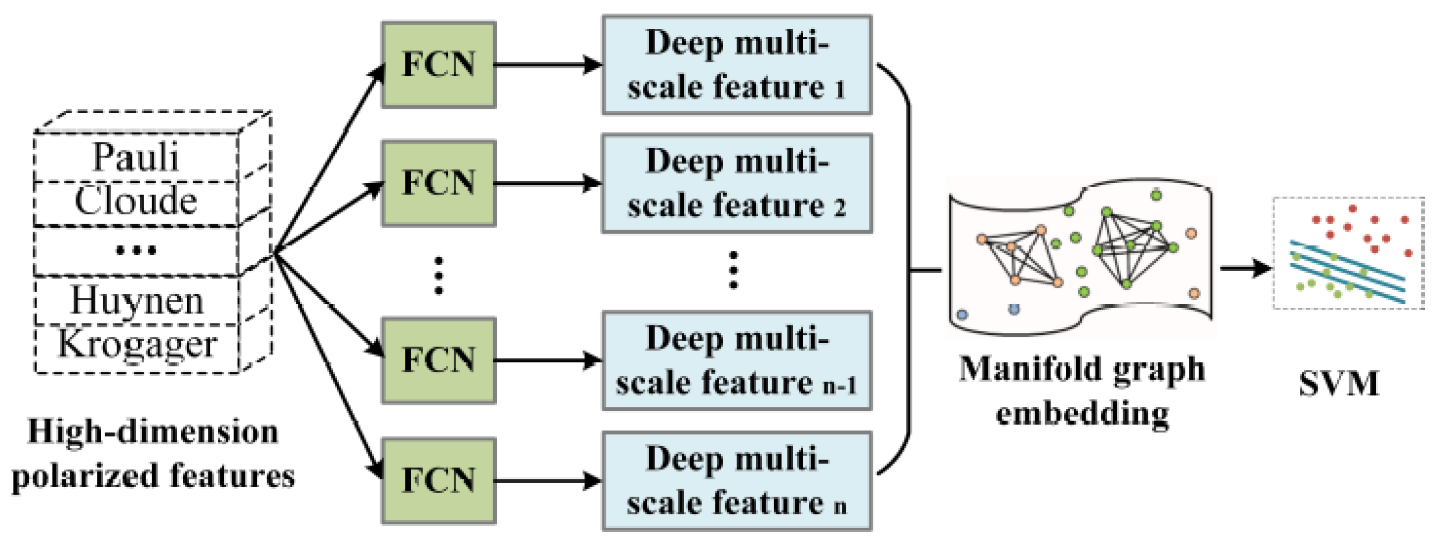
Aiming at these problems, this paper proposes a PolSAR image classification algorithm based on a multi-parallel FCN and a manifold graph embedding model. First, based on the scattering matrix and coherent matrix, high-dimensional polarized features of PolSAR data are extracted and color-coded according to different decomposition methods. Then, inspired by transfer learning, those synthesized multi-color maps are fed into the multiple-parallel FCN (MFCN) model, pre-trained on optical images, for deep multi-scale spatial feature learning. Feature maps from the last layer of the multi-parallel FCN-8s models are concatenated to generate better fused features. Finally, the manifold graph embedding model is applied to determine the effective representation of the fused feature in a low-dimensional subspace, which serves as the input of an SVM to obtain the final classification results. The main contributions of this paper are as follows:

(1)

Based on transfer learning, parallel FCN models are utilized to automatically learn deep multi-scale spatial features. Since the input of the MFCN originates from polarized features in PolSAR imagery, spatially polarized information can be adaptively fused while learning discriminative deep features.

(2)

The manifold graph embedding model explores the representation of spatially polarized fused features in a low-dimensional subspace, mining the essential structure of the PolSAR data to improve the fused feature s classification discriminability.

(3)

The proposed algorithm makes full use of the advantages of deep learning and shallow manifold graph embedding models, complementing each other to enhance the classification performance.

This article is organized as follows. Section 2 introduces the background of the multi-dimensional space of PolSAR data, the FCN structure and the graph embedding framework. In Section 3, the principle of the presented manifold graph embedding-based MFCN model for PolSAR image classification is illustrated. Section 4 describes our experimental results and corresponding detailed analysis. Finally, the conclusions of this paper are summarized in Section 5.

2. Preliminaries

2.1. Multi-Dimensional Polarization SAR Data

The polarimetric synthetic aperture radar system (PolSAR) can provide the amplitude, phase and frequency characteristics of the target scattering echo, and also takes advantage of its polarization characteristics. PolSAR can obtain the polarimetric scattering matrix of the target by measuring the polarimetric scattering characteristics of the target by transmitting and receiving different polarimetric electromagnetic waves. The polarization scattering matrix, also known as the Sinclair Matrix [27], is a 2 × 2 complex number matrix and represented by a Matrix S:

$$\left[S\right]=\left[\begin{array}{cc}{S}_{HH}& S_{HV}\\ S_{VH}& S_{VV}\end{array}\right]$$

(1)

$$S_{ij}=\left|S_{ij}\right|\frac{e^{i{k}_{0}r}}{r},i,j\in \{H,V\}$$

(2)

where H stands for Horizontal Polarization and V means Vertical Polarization. Element $S_{xy}$ represents the complex scattering coefficient when the emission polarization is y and the receiving polarization is x, while $S_{HH}$ and $S_{VV}$ denote the co-polarization components while $S_{HV}$ and $S_{VH}$ are the cross-polarization components. r denotes the distance between the terrain target and the PolSAR system and $k_0$ is the coefficient of the electromagnetic wave emitted by the PolSAR system.

The matrix unifies the phase, energy and polarization characteristics of the target and describes the electromagnetic scattering characteristics of the radar target relatively completely.

In the actual scene radar measurement, the SAR data show a certain degree of randomness. To suppress the speckle noise’s interference, it is necessary to use statistical methods to analyze the electromagnetic scattering characteristics of the target. The commonly used second-order statistic, the polarization coherence matrix T, is shown in the formula below:

$$T=〈k_p·k_p^{\mathrm{H}}〉=\frac{1}{n}\sum _{i=1}^n{\overrightarrow{k}}_P{\overrightarrow{k}}_P=\left[\begin{array}{ccc}{T}_{11}\hfill & T_{12}\hfill & T_{13}\hfill \\ T_{21}\hfill & T_{22}\hfill & T_{23}\hfill \\ T_{31}\hfill & T_{32}\hfill & T_{33}\hfill \end{array}\right]$$

(3)

where $T_{ij}$ is the element of a polarized coherence matrix T and $k_p$ is the target vector of polarized scattering matrix S under a Pauli basis:

$$k_p=\frac{1}{\sqrt{2}}{\left[S_{HH}+S_{VV},S_{HH}-S_{VV},2S_{HV}\right]}^T$$

(4)

For the better interpretation of PolSAR data, many target polarimetric decomposition methods have been developed, such as Yamaguchi decomposition [28], Huynen decomposition and so on. In practice, different polarization decomposition methods are suitable for different objects. A reasonable method is to combine the polarization characteristics of different types of target decomposition to describe PolSAR data. Therefore, this paper adopts coherent features based on a scattering matrix S, statistical features based on a coherence matrix T and polarized incoherence features to represent PolSAR images.

2.2. Fully Convolutional Networks

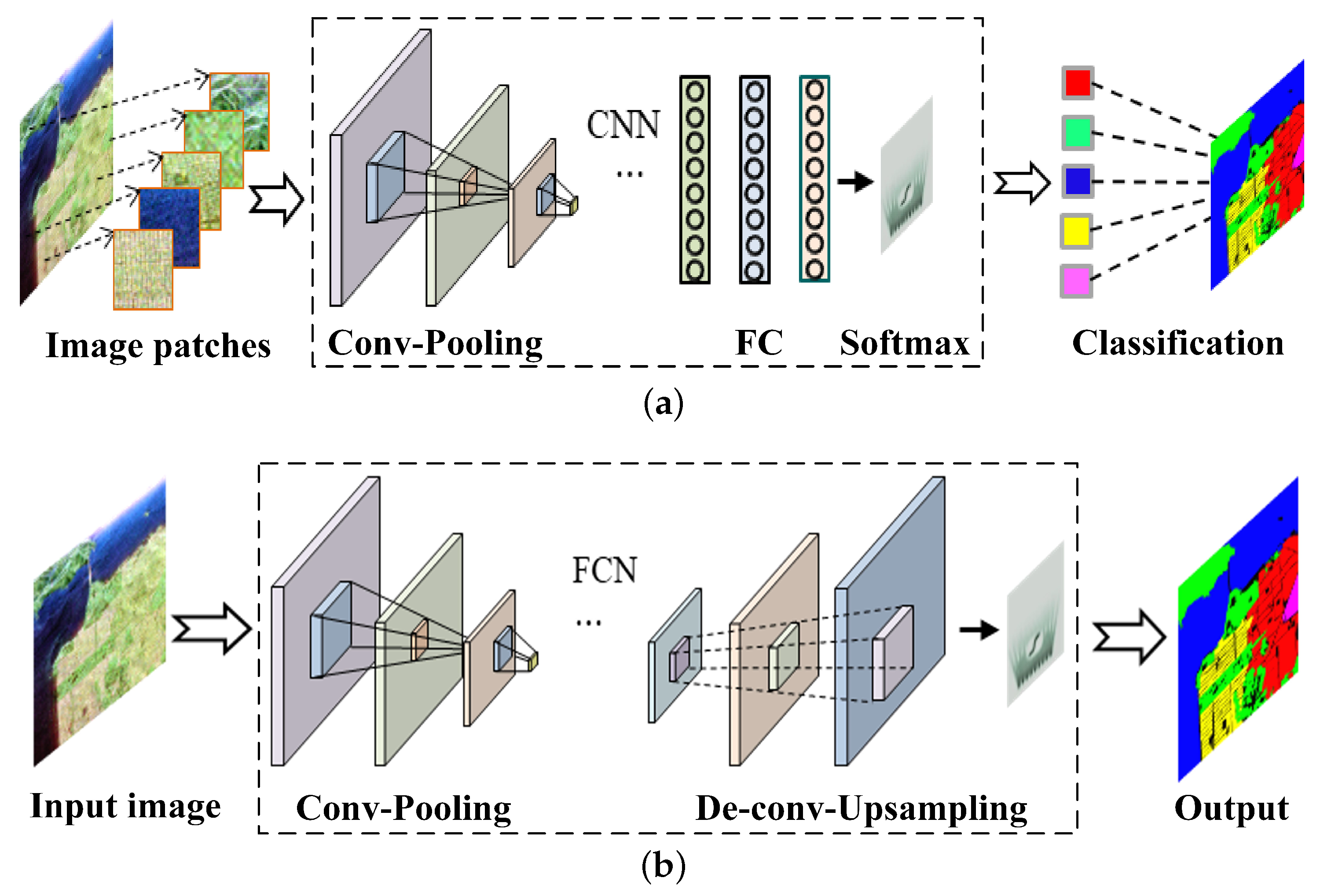
FCN [21] solves the problem of semantic segmentation by performing pixel-level classification of images. Traditional CNNs use fully-connected layers to obtain fixed-length feature vectors for classification after convolutional layers. As a pioneer of image semantic segmentation, FCN is different from classic CNN in that it can accept input images of any size. By using a deconvolution layer to upsample the feature map of the last convolution layer to restore it to the same size as the input image, a prediction can be generated for each pixel while retaining the space in the original input image Finally, the softmax classification loss is calculated pixel by pixel on the upsampled feature map, which is equivalent to each pixel corresponding to a training sample.

FCN can basically locate the target area through convolution and deconvolution. However, in the early stage of the model, the feature weight image is output through convolution, pooling and nonlinear activation function. The image output after deconvolution and other operations is actually rough and loses a lot of details. Thus, FCN needs to find a way to fill the missing details.

To further improve prediction performance, FCNs use skip structure to fuse information at different layers. There are three different structures: FCN-32s, FCN-16s and FCN-8s. Their difference lies in the number of feature fusions. FCN-8s, as shown in Figure 1, performs feature fusion between three layers of feature maps. It has been proved to have the best semantic segmentation performance in theory and practice. That is, multi-layer feature fusion helps to improve accuracy. This is because the shallow layer can extract local linear features of the image, while the deep layer can learn global semantic features. Therefore, the final feature map has strong expression ability. Based on this, this paper uses FCN-8s to learn the multi-scale deep space features of PolSAR images.

2.3. Graph Embedding Framework

Graph embedding transforms data denoted by graph into subspace representation in a low dimension and retains the graph’s structure and characteristics to the maximum extent [29]. The unified dimensionality reduction framework based on graph embedding was first proposed by Yan’s team [30], and they used an undirected weighted graph to represent the similarity between different data.

Considering that $X_1,X_2,\dots ,X_m$, $X_i\in R^n$ indicates m data points in an n-dimensional space, dimensionality reduction aims to seek a set of representations $y_1,y_2,\dots ,y_m$, $y_i\in R^k$ in a low-dimensional subspace with k dimensions, so that $y_i$ can stand for $X_i$. Under the graph embedding framework, given a graph $G=\{X,W\}$ with m nodes, $X={\left\{x_i\right\}}_{i=1}^m$ indicates m vertices of the graph and W is a $m\times m$ symmetric matrix, whose element $W_{ij}$ is defined as similarity between connected samples $x_i$ and $x_j$.

The purpose of graph embedding is to find a mapping matrix $Q\in R^{n\times k}$, which maps the original data X to y in low-dimensional space by $y=Q^{T}X$ and preserves the similarity between vertex pairs. For good embedding, two similar data points should be as compact as possible in the low-dimensional subspace; if they are embedded far apart, a larger "penalty" should be imposed. Therefore, in the graph embedding model, an intrinsic graph and a penalty graph are constructed to represent attributes we want to retain and suppress in the low-dimensional subspace, respectively. In the intrinsic graph, if two samples are the k-nearest neighbors belonging to the same class, they are connected. In the penalty graph, the connection is made only if the two samples belong to different classes. The unified objective function of the graph embedding algorithm is as follows:

$$\underset{y^{T}Ay=c}{argmin}\sum _{i\ne j}{∥y_i-y_j∥}^2{W}_{ij}$$

(5)

Through simple algebraic operations (for a detailed derivation, see [31]), it can be further formulated as follows:

$$Q^{T}X{L}^I{X}^{T}Q,\mathrm{s}.\mathrm{t}.Q^{T}XA{X}^{T}Q=c$$

(6)

$L^I$ denotes the Laplacian matrix of the intrinsic graph. A is a diagonally constrained matrix for scale normalization, which is usually valued as a Laplacian matrix $L^P$ of the penalty graph. c is a constant and usually takes a value of 1. Through the formulas above, the optimal mapping matrix can be obtained:

$$Q^{\ast }=\underset{Q}{argmin}\frac{\left|Q^{T}X{L}^I{X}^{T}Q\right|}{Q^{T}X{L}^P{X}^{T}Q}$$

(7)

According to the formulas above, the difference in the dimensionality reduction algorithms based on graph embedding is mainly rooted in Laplacian matrices $L^I$ and $L^P$ corresponding to the intrinsic and penalty graphs, respectively. Generally, the Laplacian matrix of the penalty graph is fixed. Therefore, the essential difference between different graph embedding algorithms lies in the design of the similarity matrix $W^I$, which will play a decisive role in the effect of dimensionality reduction.

3. Proposed Method

3.1. The Proposed Algorithm Framework for PolSAR Image Classification

Considering that the FCN-8s model has a variety of receptive fields with different sizes, it can perceive the object’s structure information at multiple scales and layers. In addition, as a traditional manifold method, the locality preserving projection (LPP) model based on graph embedding can significantly preserve the original data’s local characteristics and deal with high-dimensional data located in manifold space well. Therefore, in our experiments, the LPP and MFCN models are integrated, and their advantages are complementarily utilized to classify PolSAR images. The proposed algorithm framework is shown in Figure 2. First, seven “RGB” synthetic pseudo-color maps are obtained through different polarized decomposition methods. After different color encodings, they are input into the pre-trained FCN-8s model. When the network automatically learns the spatial information of adjacent pixels, the polarized properties can be adaptively fused with the spatial structure. In this case, the MFCN can extract features at different network levels. Since the same pre-trained FCN-8s model in the MFCN is adopted as a feature extractor, there is redundancy in the spatially polarized fused features extracted by the MFCN. To remove redundant information in the cascaded features with high dimensionality, the manifold algorithm LPP based on graph embedding is utilized for dimensionality reduction before the final classification. Considering that features learned by the MFCN are already sparse and nonlinear, this work combines the manifold graph embedding model LPP to remove redundancy in high-dimensional features to capture the most essential data structure, which is finally fed into a classifier to obtain the classification results. Considering that SVM is a trainable classifier and its nonlinear kernel function can better distinguish complex image features, our method uses the most commonly used SVM as the classifier.

3.2. Feature Learning Based on an MFCN

CNN-based classification methods are usually based on image patches, whose appropriate size is difficult to determine. In addition, to classify each pixel, a pixel-by-pixel sliding window strategy is necessary. However, it will lead to many repeated operations, greatly increasing the computational time and required storage space. Therefore, this paper utilizes an FCN for pixel-level PolSAR image classification, as shown in Figure 3. Since the scale of PolSAR data is quite small, retraining the network from scratch is not realistic. Therefore, the transfer-learning strategy is considered to migrate the FCN model (pre-trained on the PASCAL VOC dataset) to learn the deep multi-scale spatial features of the PolSAR images [32]. Considering the sample capacity of the PolSAR dataset and its differences from one of optical images, and the similarity of PolSAR images and optical images is small, a reasonable method is to use the FCN model pre-trained on the optical image as a feature extractor to get deep spatial features of PolSAR images and then uses a classifier to perform final classification. In the experiments, an FCN is employed as a feature extractor when some of the underlying layer parameters are fine-tuned.

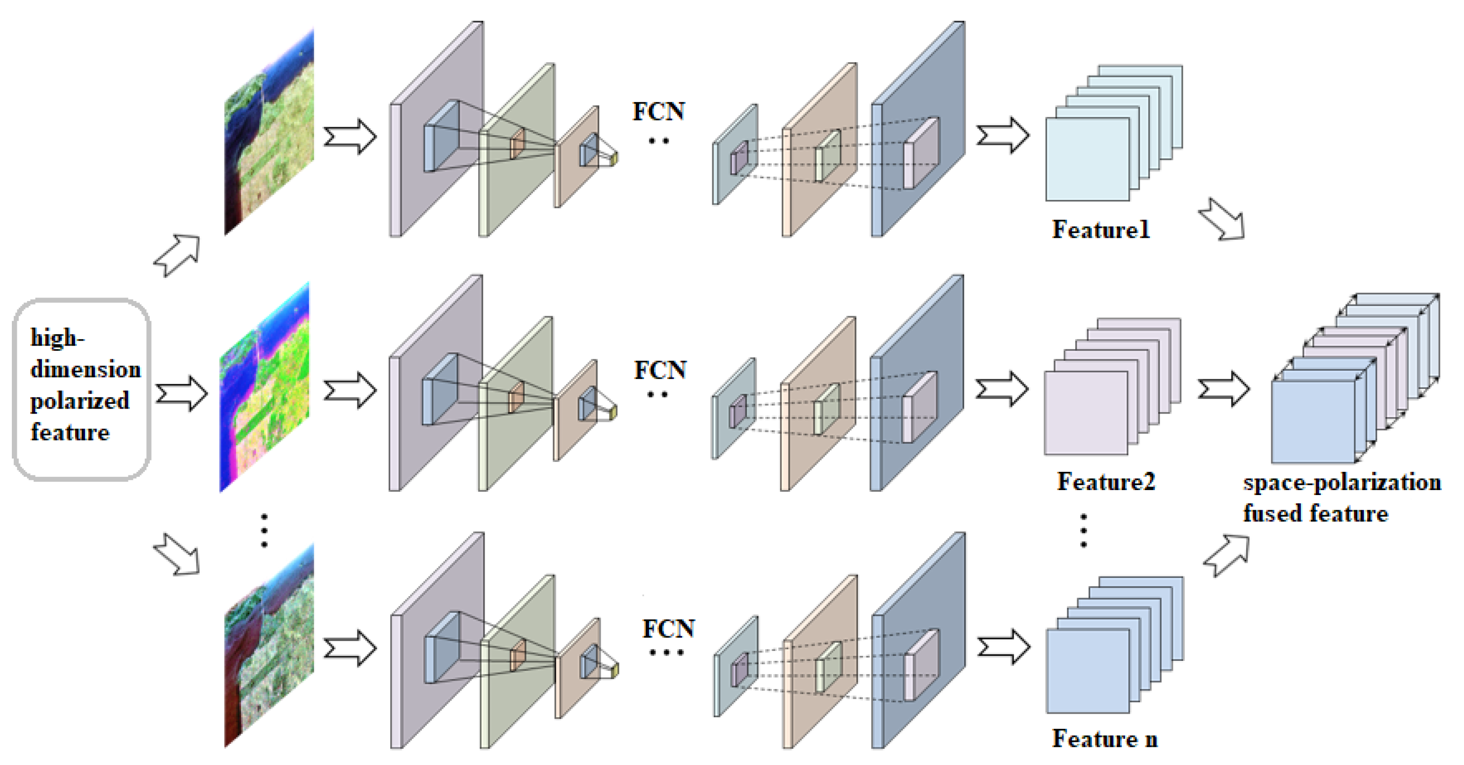
There are many targets with different scattering characteristics in real scenes, and to make the spatially polarized features represent different objects more effectively, this paper proposes a multiple-parallel FCN-8s (MFCN) model for feature learning and fusion of PolSAR images, as shown in Figure 4. Various polarized decompositions are fed into different FCN-8s models, and the final spatial feature maps are cascaded into high-dimensional features for PolSAR imagery representation. According to our previous research [31], it is obvious that, for the same network input, e.g., Pauli decompositions, each filter in the score layer outputs different feature maps, which means that different filters prefer different object types. In addition, for different network inputs, the same filter at the same network layer can obtain different feature maps, mainly depending on different polarized information inputs. In this respect, spatially polarized fused features from the proposed MFCN can be helpful in distinguishing different types of terrain objects.

3.3. Dimensionality Reduction Based on Manifold Graph Embedding

Nonlinear data with high dimensions are usually compactly distributed in a low-dimensional manifold space; therefore, it is necessary to explore the most intrinsic data structure using manifold algorithms. The objective functions of global manifold methods (ISOMAP) and local manifold techniques (LLE and LE) all involve a Laplacian matrix and are eventually transformed into eigenvalue decomposition problems. However, these nonlinear methods have common drawbacks: the mapping of the original high-dimensional data to a low-dimensional subspace has no explicit functional expression.

To solve the problem of external samples, this paper adopts the locality preserving projection (LPP) [33], which can be regarded as a linear approximation of the nonlinear LE method. As a manifold dimension reduction model based on graph embedding, the LPP algorithm can restore nonlinear manifolds important properties by retaining local structures. The LPP algorithm includes three main steps: construction of adjacency graphs, assignment of weights and calculation. The detailed process is as follows:

Stage 1: There are two strategies to measure the ”similarity” in adjacency graphs. The first is the $\epsilon$-nearest neighbor: if ${\left|\right|x_i-x_j\left|\right|}^2<\epsilon$, then node i is connected to node j. The second strategy is the k-nearest neighbor: if node i is the k-nearest neighbor of node j, then the two nodes are connected. Relatively speaking, the k-nearest neighbor is widely used because of its stability, but it has a higher time cost [34]. The $\epsilon$-nearest neighbor is suitable for scenarios with high computational complexity, but it is very difficult to select an optimal $\epsilon$ in real applications. To construct a stable graph and make full use of existing label information to enhance feature discriminability, this paper chooses the k-nearest neighbor method to generate the graph.

Stage 2: There are two strategies in Stage 2: the thermonuclear method and the simple method for weight distribution. If node i and node j are connected, then the weight is $W_{ij}$; otherwise, the weight is 0. For the simple method, the allocation of weights does not involve parameters. Only when node i and node j are connected, the $W_{ij}$ is 1; otherwise, it is 0. For connected nodes, this paper utilizes a thermonuclear strategy to distribute the weights as follows:

$$\begin{array}{c}{W}_{ij}=\left\{\begin{array}{c}{e}^{-\frac{{∥x_i-x_j∥}^2}{t}},\mathrm{if}\mathrm{label}\left(x_i\right)=\mathrm{label}\left(x_j\right)\mathrm{and}\\ x_i\in N_k\left(x_j\right)\mathrm{or}{x}_j\in N_k\left(x_i\right)\\ 0,\mathrm{otherwise}\\ \mathrm{s}.\mathrm{t}.W_{ii}=0\end{array}\right.\end{array}$$

(8)

When the value of $\epsilon$ or k is infinite and the eigenvector corresponding to the maximum eigenvalue is selected, the data will be mapped along the direction of the maximum covariance to preserve the global structure; otherwise, local characteristics will be maintained.

Stage 3: In this stage, eigenvectors are calculated by generalized eigenvalue decomposition:

$$XL{X}^{T}Q=\lambda XD{X}^{T}Q$$

(9)

where D is a diagonal matrix and $L=D-W$ is a Laplacian matrix. Considering that ${\lambda }_1<{\lambda }_2<\dots {\lambda }_n$ denote eigenvalues arranged from smallest to largest and column vectors $q_0,q_1,\dots ,q_n$ represent the corresponding eigenvectors, the embedding of the LPP can be expressed as:

$${\mathrm{x}}_i\to {\mathrm{y}}_i=Q_{LPP}^T{\mathrm{x}}_i,Q_{LPP}=\left(q_1,q_2,\cdots q_k\right)$$

(10)

where $Q_{LPP}$ is a transformation matrix with a size of $n\times k$ and each column represents an embedding of the LPP in manifold space. To a certain extent, the local neighborhood information of the data is effectively preserved.

Moreover, to solve the singular value problem, this paper uses a regularization strategy according to the idea in [35], adding a constant value to every diagonal element in matrix $XD{X}^T$. For any regularization parameter $\phi$, $XD{X}^T+\phi I$ (I is a unit matrix) is a nonsingular matrix when $\phi >0$. Therefore, by solving the eigenvalue decomposition problem with the regularization term, the first k eigenvectors corresponding to the eigenvalues (arranged from smallest to largest) are selected to form the manifold mapping matrix $Q_{LPP}^{\ast }$.

$$Q_{LPP}^{\ast }=\underset{Q}{argmax}\frac{\left|Q^{T}XW{X}^{T}Q\right|}{Q^{T}XD{X}^{T}Q+\phi I}$$

(11)

Finally, the representation of PolSAR data $Y_{LPP}$ in the low-dimensional manifold subspace can be obtained by the linear mapping function $Y_{LPP}=Q_{LPP}^{T}X$, which well retains the local intrinsic characteristics of the original data.

4. Experiments and Analysis

Experiments were carried out on three typical datasets. The performance of the MFCN+LPP algorithm was quantitatively and qualitatively compared with the standard FCN- and LPP-based approaches. The discussion and analysis are presented in this section.

4.1. Experiments Data

To validate the effectiveness of the proposed classification scheme, we conducted extensive experiments on three classic PolSAR datasets for quantitative and qualitative comparison with other existing algorithms. The ground truth images of Flevoland Dataset 1 and San Francisco dataset are generated by manual annotation according to the associated optical image, which can be found in the Google Earth by the information provided in the metadata files.

(1)

$Flevol$ and $Dataset$ 1: These data were obtained in the Netherlands by the AIRSAR system of the NASA Jet Propulsion Laboratory in 1989. As a four-look fully polarized image of the L-band, its image size is $750\times 1024$ pixels, and the resolution of the distance and azimuth are 6 and 12 m, respectively. According to Wang et al. [31], the whole scene has been divided into 11 species: rapeseed, grass, forest, peas, lucerne, wheat, beets, bare soil, stem beans, water and potatoes. This fully PolSAR image, a classic farmland dataset, has been widely used to verify pixel-level classification performances. Its Pauli pseudo-color map, corresponding ground truth and labels are shown in Figure 5, and the pixel number of each class is given in the bracket of label image.

(2)

$San$$Francisco$$dataset$: This dataset is a four-look fully polarized image of the L-band, collected by NASA Jet Propulsion Laboratory’s AIRSAR system in the San Francisco Bay Area. The image size is $900\times 1024$ pixels, and its spatial resolution is approximately 10 m × 10 m. As shown in the Pauli image and ground truth in Figure 6, there are three major types of objects, namely vegetation, sea and urban areas, the latter being further divided into high-density urban areas, developed urban areas and low-density urban areas.

(3)

$Flevol$ and $Dataset$ 2: The third fully polarized SAR image adopted in this paper is also L-band AIRSAR data collected in Holland in 1991. The number of looks from the dataset is four, and the image of size $1024\times 1024$ pixels contains only farmland areas. The scene consists of 14 crops: potatoes, fruit, oats, beet, barley, onions, wheat, beans, peas, maize, flax, rapeseed, grass and lucerne. Comprising a rich variety of geometric species with similar scattering characteristics, it is of great significance for this image to be utilized for verifying the proposed classification algorithm. Figure 7 shows the Pauli RGB map and the corresponding ground truth, as suggested by Zhang et al. [36].

4.2. Experimental Settings and Parameter Tuning

$\left(1\right)$$Experimental$$settings:$ In the experiments, our datasets were all processed by multi-looking process, which is a basic method for speckle suppression of SAR images. Drawing on transfer learning, different pseudo-color maps were first fed into pre-trained multiple-FCN8s (MFCN) models to learn the multi-scale deep spatial features automatically. During this process, polarization characteristics and spatial information could be adaptively fused. Then, the outputs of the last layer from each FCN-8s were stacked to form spatially polarized fused features. For high-dimensional fused features (the labels are known in advance), a certain proportion of them was randomly selected as the training set, and the remaining selected for testing. The training set was utilized to construct an intrinsic graph and a penalty graph to learn the mapping relationship (represented by a matrix Q) from a high-dimensional feature space to a manifold subspace. Finally, an SVM classifier with a Gaussian kernel was trained to obtain the final classification results on the test samples.

To robustly evaluate the classification performance of the proposed algorithm, the overall accuracy (OA), kappa coefficient, and confusion matrix are employed as evaluation indicators, and comparative experiments were conducted with the following algorithms.

(a)

Local preserving projection (LPP) finds a manifold representation of polarized features in a low-dimensional subspace without considering the spatial relationship between pixels.

(b)

FCN: A single pre-trained FCN is adopted to learn the multi-scale spatial structure of the PolSAR data. This nonlinear feature is actually a deep abstract semantic representation with relatively simple polarization properties.

(c)

FCN+LPP: A single FCN extracts the multi-scale spatial features in PolSAR imagery, which undergo dimensionality reduction by the LPP algorithm for further classification.

(d)

MFCN+LPP is he algorithm proposed in this paper. First, to describe various ground objects effectively, seven polarized decompositions are fed into multiple parallel FCN-8s models to learn multi-scale deep spatial features. Afterwards, through the manifold graph embedding model (LPP), the compact manifold representation of high-dimensional spatially polarized features from the MFCN is extracted for final classification.

$\left(2\right)$$Parameter$$settings:$ The classification algorithm proposed in this paper can be divided into three stages: feature learning and fusion, dimension reduction and classification. In the first phase, there are millions of parameters in the FCN model to be learned. Considering the cost and scarcity of PolSAR data, this paper draws on transfer learning and employs FCN-8s, which have been pre-trained on the PASCAL VOC 2011 dataset. Good model parameters are migrated to learn the characteristics of the PolSAR data.

During this process, the original image is cut into four small patches; three of these patches are selected as the training set, and the remaining one is used for the test set. After four successive cycles, the classification results of the whole image can be obtained. Seven typical decomposition methods (Pauli decomposition, Cloude decomposition, Freeman decomposition, $H/A/\alpha$ decomposition, Huynen decomposition, Yamaguchi decomposition and Krogager decomposition) were adopted in the experiments. Pseudo-color images from some different decompositions and the corresponding constituents of the R, G, and B channels are shown in Figure 8 and

Table 1. RGB channels of different polarized decompositions.

Polarized Decompositions	R Channel	G Channel	B Channel
Pauli	2$A_0$	$B_0+B$	$B_0-B$
Cloude	$\sqrt{{\lambda }_1}\left|u_{11}\right|$	$\sqrt{{\lambda }_1}\left|u_{12}\right|$	$\sqrt{{\lambda }_1}\left|u_{13}\right|$
Freeman	$f_S\left(1+{\beta }^2\right)$	$f_D\left(1+{\alpha }^2\right)$	$\frac{8f_V}{3}$
$H/A/\alpha$	$\sqrt{\lambda }cos\left(\alpha \right)$	$\sqrt{\lambda }sin\left(\alpha \right)cos\left(\beta \right)$	$\sqrt{\lambda }sin\left(\alpha \right)sin\left(\beta \right)$
Huynen	$〈2A_0〉$	$\left({\langle C\rangle }^2+{\langle D\rangle }^2\right)/2A_0$	$\left({\langle H\rangle }^2+{\langle G\rangle }^2\right)/2A_0$
Yamaguchi	$P_D$	$P_V$	$P_S$
Krogager	$k_S$	$k_D$	$k_H$

, respectively. To accomplish this goal, seven parallel FCNs with pseudo-color images from different decompositions as input learned the multi-scale deep spatial features adaptively, achieving the simultaneous fusion of the polarized properties and spatial information.

During the second stage, dimensionality reduction is conducted based on the manifold graph embedding model, and the training set and test set are divided. According to our previous research [31], the training ratios for Flevoland Dataset 1, the San Francisco dataset and Flevoland Dataset 2 were set to 5%, 3% and 5%, respectively. In addition, when establishing the manifold graph embedding model, designing a weight matrix W and specifying a subspace dimension k also involve parameter selection. First, for a weight matrix W, a thermonuclear function ($t=1$, Tikhonov regularization with a strength of 0.1) is chosen. In addition, the curve of the classification accuracy varies with the subspace dimensionality, as shown in Figure 9. Considering both the accuracy and time consumption, the subspace dimensions k of Flevoland Dataset 1, the San Francisco dataset and Flevoland Dataset 2 were set to 90, 50 and 35, respectively.

For the final classification, an SVM with a Gaussian kernel is employed as the classifier, and we use five-fold CrossValidation to optimize the parameters. To more intuitively analyze the classification effect of the dataset on multiple comparative experimental methods in this paper, we assume that the intensity of speckle noise of the training data and test data in each dataset is consistent.

4.3. Experimental Results and Analysis

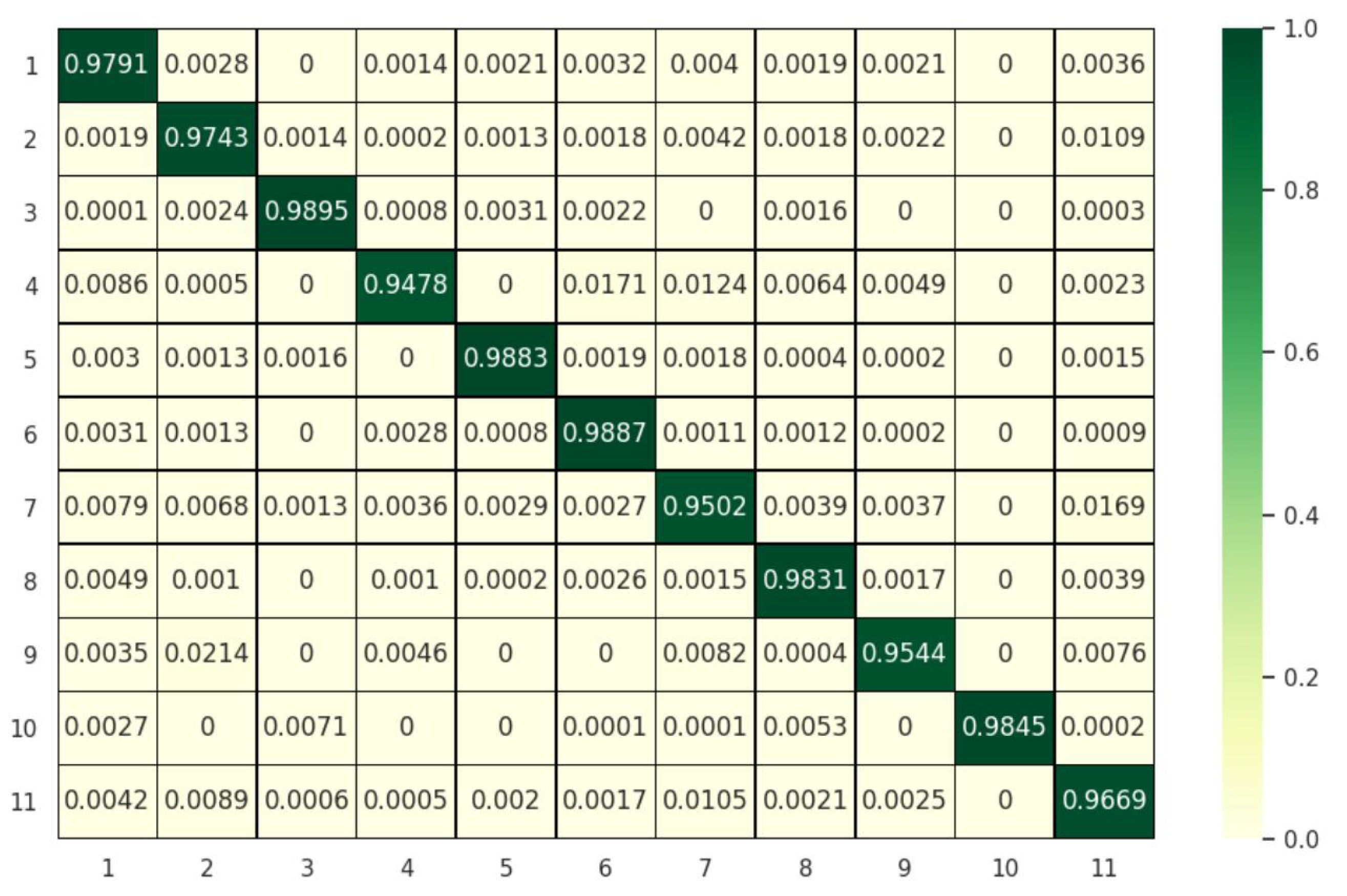
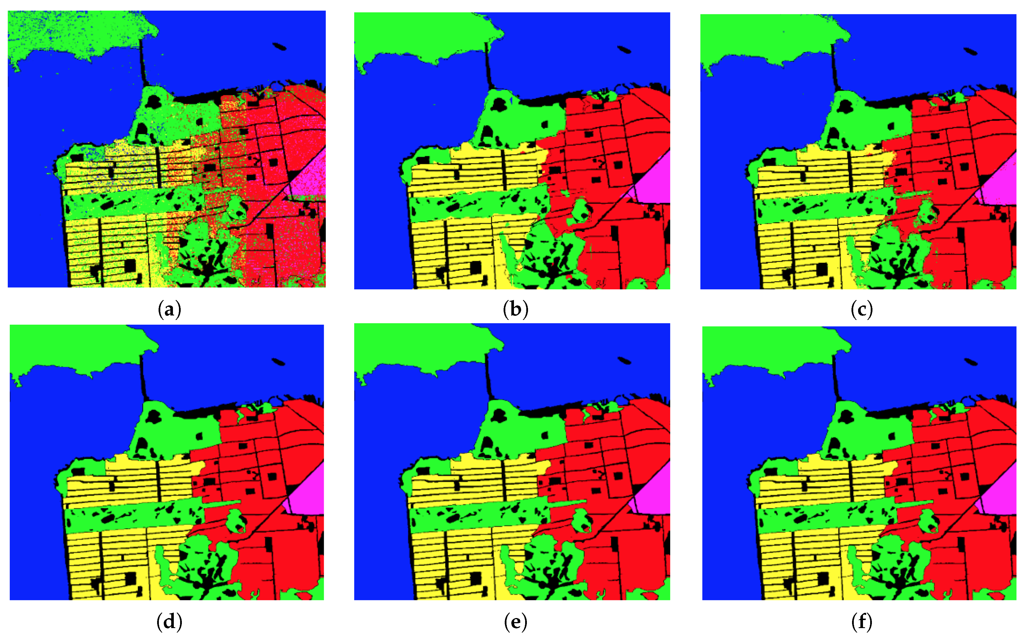
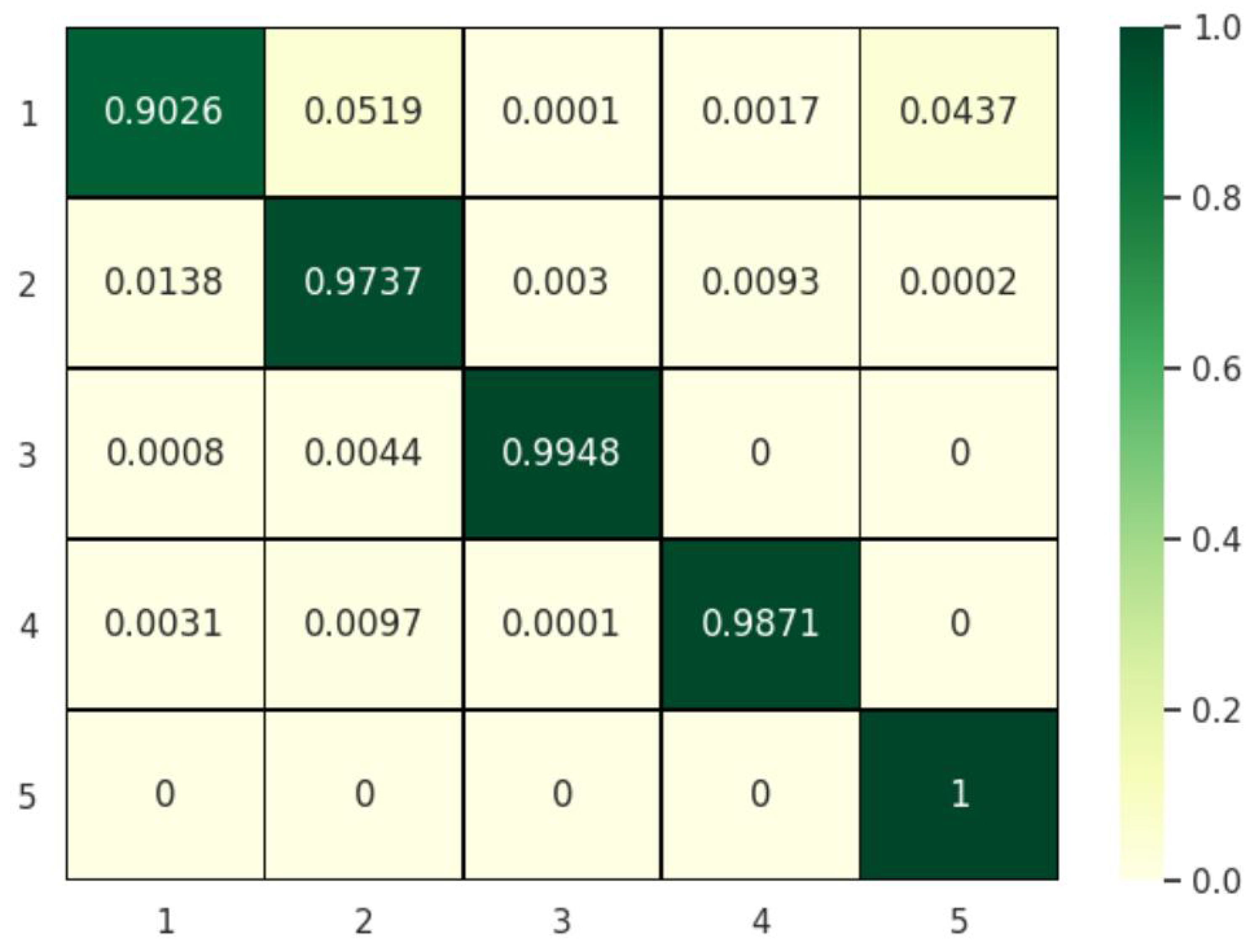
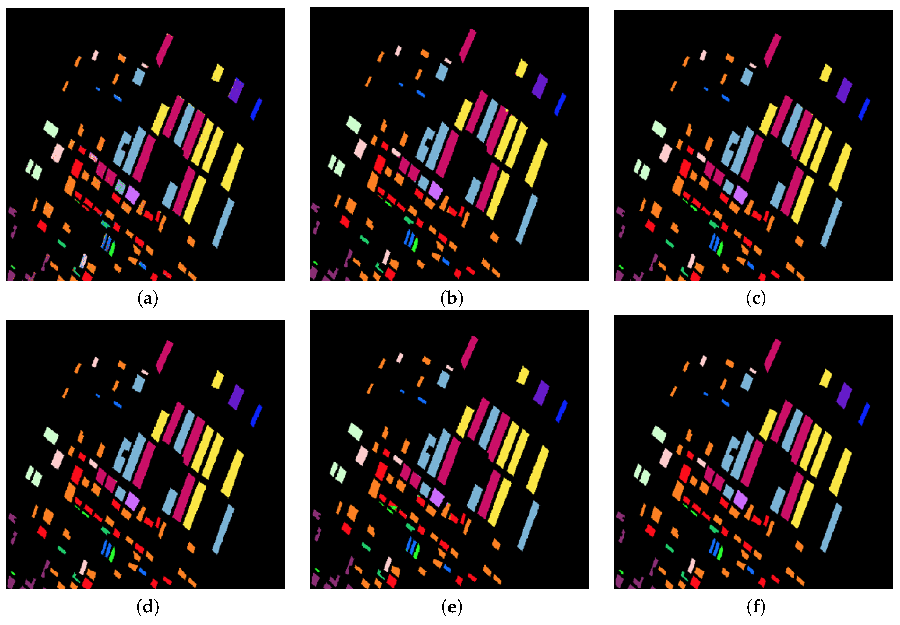
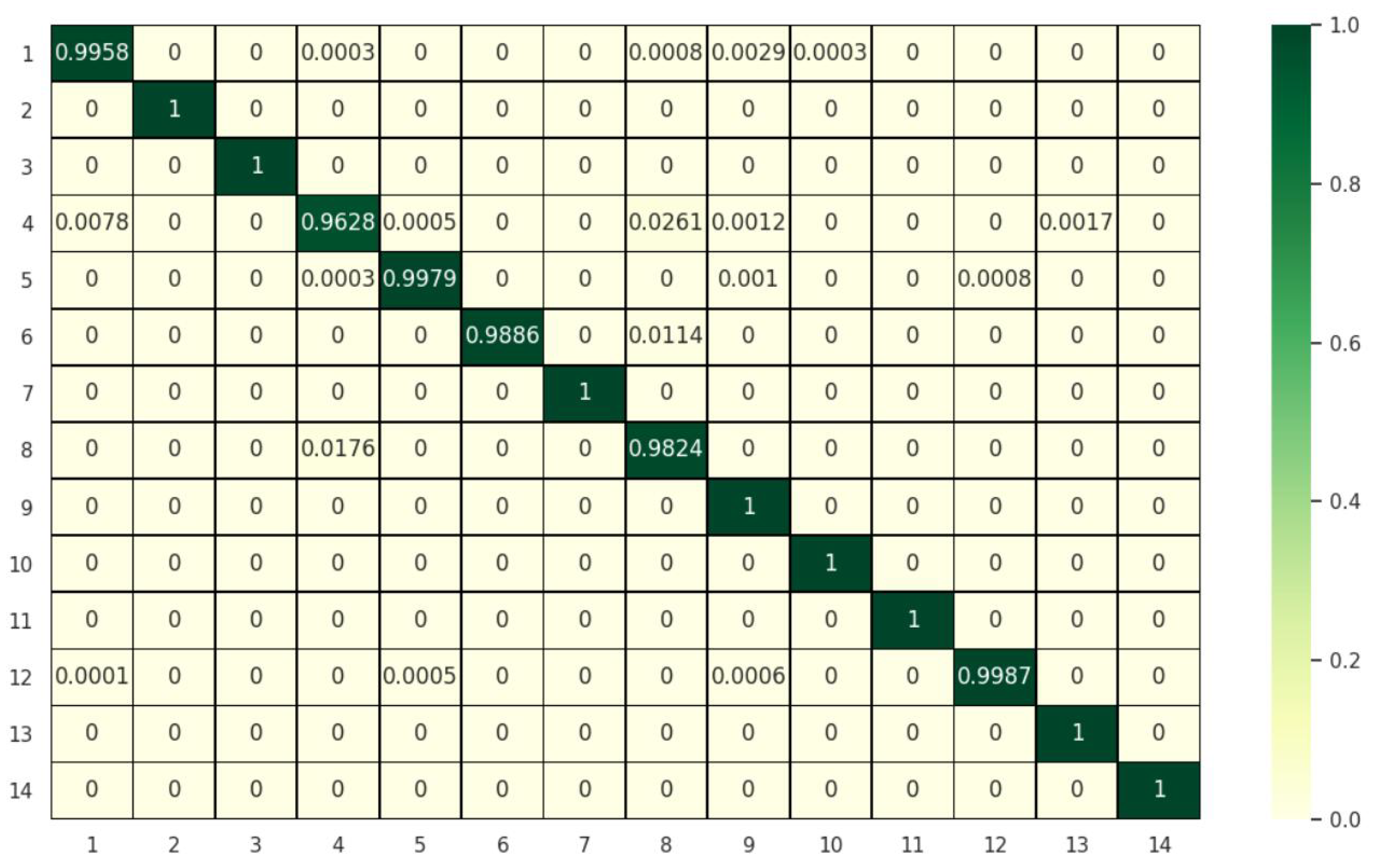
In this section, the classification results of the proposed method and comparative algorithms are described from multiple perspectives. Specifically, the corresponding classification accuracy values, OAs and kappa coefficients for the different algorithms are listed in

Table 2. OAs and kappa coefficients for the different classification methods in the Flevoland Dataset 1 (numbers in bold indicate best performance).

Label/Class	LPP	FCN	FCN+LPP	MFCN+LPP
1/Rapeseed	75.64%	89.67%	96.21%	97.91%
2/Grass	78.68%	94.68%	96.83%	97.43%
3/Forest	71.80%	97.40%	98.87%	98.95%
4/Peas	54.67%	91.87%	95.12%	94.78%
5/Lucerne	65.07%	92.98%	96.64%	98.83%
6/Wheat	84.43%	95.03%	97.31%	98.86%
7/Beets	56.34%	77.57%	90.75%	95.02%
8/Bare soil	49.08%	95.99%	98.30%	98.30%
9/Stem beans	79.02%	71.13%	90.46%	95.43%
10/Water	97.41%	99.95%	99.95%	98.45%
11/Potatoes	77.49%	90.81%	96.09%	96.69%
$OA$	73.70%	90.99%	96.08%	97.39%
$Kappa$	70.29%	89.82%	95.57%	97.06%

,

Table 3. OAs and kappa coefficients for the different classification methods in the San Francisco Dataset (numbers in bold indicate best performance).

Label/Class	LPP	FCN	FCN+LPP	MFCN+LPP
1/Sea	79.30%	97.31%	97.98%	90.26%
2/Vegetation	88.19%	95.41%	96.68%	97.37%
3/Developed urban areas	99.53%	99.44%	99.73%	99.48%
4/High-density urban areas	77.63%	97.40%	93.29%	98.71%
5/Low-density urban areas	65.09%	97.79%	91.73%	100%
$OA$	89.37%	97.82%	98.46%	96.95%
$Kappa$	85.00%	96.93%	97.83%	95.72%

and

Table 4. OAs and kappa coefficients for the different classification methods in the Flevoland Dataset 2 (numbers in bold indicate best performance).

Label/Class	LPP	FCN	FCN+LPP	MFCN+LPP
1/Potatoes	96.28%	99.53%	99.93%	99.58%
2/Fruit	94.56%	99.85%	99.91%	100%
3/Oats	96.15%	100%	100%	100%
4/Beets	97.85%	98.31%	99.81%	90.28%
5/Barley	97.25%	99.90%	99.82%	91.79%
6/Onions	77.55%	99.80%	99.01%	98.86%
7/Wheat	98.93%	99.78%	99.90%	100%
8/Beans	56.39%	90.54%	98.36%	98.24%
9/Peas	99.27%	99.27%	99.90%	100%
10/Maize	86.45%	99.27%	99.35%	100%
11/Flax	99.68%	100%	100%	100%
12/Rapeseed	98.66%	99.52%	99.81%	99.86%
13/Grass	84.79%	98.65%	99.57%	100%
14/Lucerne	91.41%	100%	100%	100%
$OA$	96.54%	97.45%	99.83%	99.54%
$Kappa$	95.92%	96.53%	99.80%	95.46%

; the confusion matrix and visualized classification results of the proposed method are shown in Figure 10, Figure 11, Figure 12, Figure 13, Figure 14 and Figure 15.

Table 2 shows that the LPP method has poor classification performance for all classes, with an average overall accuracy of 73.70%. The main reason is that the LPP algorithm is a shallow learning algorithm and lacks spatial constraints. The classification accuracy of the FCN has been greatly improved for all categories (OA of 90.99%) except 71.13% in Category 9, which is lower than that of the LPP algorithm. By contrast, with the FCN+LPP algorithm, the complementation of deep spatial features by the FCN and manifold graph embedding learning can greatly enhance the classification accuracy in most categories. Especially for rapeseed, beets and stem beans, the corresponding accuracy has been improved 6%, 13% and 19%, indicating that manifold subspace representation has gained deep multi-scale spatial features.

Compared with the FCN+LPP algorithm, the accuracy of the MFCN+LPP algorithm for almost every category has been improved, especially on beets and stem beans (5% for both). This finding demonstrates that polarized property passes through the presented MFCN, and fusions with multi-scale spatial features can be more effective for pixel-level classification.

For the San Francisco dataset, the experimental results in Table 3 show that the performance of the FCN+LPP algorithm is higher than that of the single LPP or FCN method. Looking at the accuracy only, the FCN outperforms the LPP algorithm, the former’s classification accuracy is greater than 95% for all categories and 99.44% for sea, which proves that spatial features from the FCN play a leading role in distinguishing different ground objects. However, according to the visualized classification results presented in Figure 12b, it is obvious that the boundary areas have many misaligned pixels. For example, there are some misclassified samples in the intersection of categories indicated by yellow and green since the FCN cannot handle edge details well.

By integrating spatial features from the FCN and manifold representations from the graph embedding model, the LPP algorithm’s advantage of retaining local characteristics can largely compensate for the FCN’s defects. After combining the FCN and LPP methods, the overall accuracy reaches 98.46%. In the proposed algorithm, the MFCN+LPP algorithm further combines polarized information with spatial features through multi-parallel convolutional neural networks; then, the manifold graph embedding model is employed to remove redundancies, and the classification accuracy of vegetation, high-density areas and low-density areas continues to grow. Moreover, the OA of the low-density areas reaches 100%, indicating that multi-scale polarized spatial features have a strong discriminating ability for classification. However, the accuracy of sea and developed areas is lower than that of the FCN+LPP method; these two categories account for a large proportion of the area; thus, the proposed method’s performance is not as good as that of the FCN+LPP method.

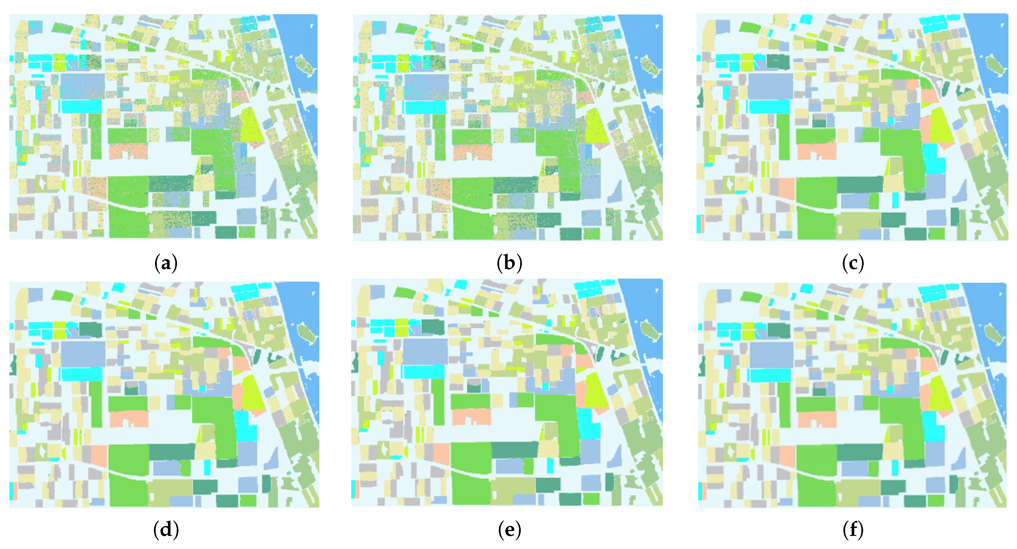
Figure 14 shows the visualized classification results of different algorithms on Flevoland Dataset 2. The corresponding OAs and kappa coefficients for each class are given in Table 4. Although the LPP-based manifold method can obtain an OA up to 96.54%, the combination of the FCN and LPP methods achieves a better performance, with the OA increasing to 99.83% (FCN+LPP) and 99.54% (MFCN+LPP).

Compared with the single LPP method (56.39% for beans), the accuracy of both the FCN+LPP and MFCN+LPP methods on the same class increased by nearly 42%. For fruit, oats, wheat, peas, maize, flax, rapeseed, grass and lucerne, the MFCN+LPP algorithm achieves the best performance on both the visualization and classification accuracy. The overall accuracy for most of the categories mentioned above is 100% except 99.86% for rapeseed. The single FCN already has excellent classification performance with an OA as high as 97.45%, but its synergy with the LPP algorithm can boost the final results. More importantly, when polarized features are fed into the MFCN, the polarization information can effectively fuse with the spatial characteristics at multiple scales and levels, thereby improving the representation ability and discrimination ability of the extracted features. Finally, the runtime of the proposed algorithm and the other comparison methods are given in

Table 5. Time consumed by feature learning and fusion of the mfcn on the three datasets (seconds/s).

Dataset	Flevoland Dataset	San Francisco Dataset	Flevoland Dataset
Image size	750 × 1024	900 × 1024	1024 × 1024
Number of parallel networks	7	7	7
Time consumption	423.08	490.98	559.86

and

Table 6. Time needed for classification by the different algorithms on the three datasets (seconds/s).

Dataset	LPP	FCN	FCN+LPP	MFCN+LPP
Flevoland Dataset 1	31.3375	14.37	28.2472	33.4559
San Francisco dataset	21.8552	13.99	20.7372	29.3127
Flevoland Dataset 2	11.1774	11.83	13.3515	18.5695

. Among them, the experiments based on the FCN-8s models for deep multi-scale spatial feature extraction were conducted in the Caffe framework using an NVIDIA Tesla K40 GPU, which took 423.08, 490.98 and 559.86 s in Flevoland Dataset 1, the San Francisco dataset and Flevoland Dataset 2, respectively, which are approximately linear with the input image size. When the hardware conditions are satisfied, parallel operations can be performed on a machine with multiple GPUs to reduce the time consumption. Other experiments were performed using MATLAB 2014 on a computer with an Intel Core i5-4570 CPU and 32 GB RAM. Table 6 indicates that the single FCN and the FCN+LPP algorithm have lower time costs, while the time consumption of the MFCN+LPP algorithm is the highest because the generated feature space of the MFCN+LPP algorithm has the highest dimensions, increasing the computational complexity.

5. Conclusions

In this paper, to effectively describe terrain with various ground object types, we propose a parallel and multi-level fully convolutional neural network for PolSAR imagery classification. For better spatial-feature learning and fusion with polarized information, the network incorporates a shallow manifold embedding subspace representation to remove redundancies. In terms of the classification accuracy, the proposed algorithm can achieve results comparable to the state-of-the art algorithm, without the need for post-processing. Furthermore, the proposed algorithm is quite fast and efficient in small datasets. The effectiveness of the proposed algorithm mainly depends on the following aspects: (1) the FCN has the powerful potential to learn automatically nonlinear deep multi-scale spatial features, and the skip architecture in the network handles pixel-level classification well; (2) subspace learning based on manifold embedding can largely preserve local features and reveal the most essential structure of PolSAR data; and (3) the deep MFCN and shallow LPP algorithms can complement each other and improve the representation and discrimination ability of the spatially polarized features. Relatively speaking, the proposed method requires more time to train the network in the phase of feature extraction, unless a machine that supports parallel computing is used. This shortcoming is also one of the problems we want to improve upon in the future. In addition, phase information has also been proven to be meaningful for characterizing ground objects in many studies, but existing network architectures are usually designed for real values as input. However, we will still attempt to combine phase information contained in PolSAR imagery to boost classification performance.

References

1. Niu, X.; Ban, Y. An adaptive contextual SEM algorithm for urban land cover mapping using multitemporal high-resolution polarimetric SAR data. IEEE J. Sel. Top. Appl. Earth Obs. Remote Sens. 2012, 5, 1129–1139. [Google Scholar] [CrossRef]
2. Van Zyl, J.J. Unsupervised classification of scattering behavior using radar polarimetry data. IEEE Trans. Geosci. Remote Sens. 1989, 27, 36–45. [Google Scholar] [CrossRef]
3. Cloude, S.R.; Pottier, E. An entropy based classification scheme for land applications of polarimetric SAR. IEEE Trans. Geosci. Remote Sens. 1997, 35, 68–78. [Google Scholar] [CrossRef]
4. Kong, J.; Swartz, A.; Yueh, H.; Novak, L.; Shin, R. Identification of terrain cover using the optimum polarimetric classifier. J. Electromagn. Waves Appl. 1988, 2, 171–194. [Google Scholar]
5. Wang, S.; Liu, K.; Pei, J.; Gong, M.; Liu, Y. Unsupervised classification of fully polarimetric SAR images based on scattering power entropy and copolarized ratio. IEEE Geosci. Remote Sens. Lett. 2012, 10, 622–626. [Google Scholar] [CrossRef]
6. Lee, J.S.; Grunes, M.R.; Ainsworth, T.L.; Du, L.J.; Schuler, D.L.; Cloude, S.R. Unsupervised classification using polarimetric decomposition and the complex Wishart classifier. IEEE Trans. Geosci. Remote Sens. 1999, 37, 2249–2258. [Google Scholar]
7. Dabboor, M.; Collins, M.J.; Karathanassi, V.; Braun, A. An unsupervised classification approach for polarimetric SAR data based on the Chernoff distance for complex Wishart distribution. IEEE Trans. Geosci. Remote Sens. 2013, 51, 4200–4213. [Google Scholar] [CrossRef]
8. Lee, J.S.; Grunes, M.R.; Kwok, R. Classification of multi-look polarimetric SAR imagery based on complex Wishart distribution. Int. J. Remote Sens. 1994, 15, 2299–2311. [Google Scholar] [CrossRef]
9. Xing, X.; Ji, K.; Zou, H.; Sun, J. Feature selection and weighted SVM classifier-based ship detection in PolSAR imagery. Int. J. Remote Sens. 2013, 34, 7925–7944. [Google Scholar] [CrossRef]
10. Feng, J.; Cao, Z.; Pi, Y. Polarimetric contextual classification of PolSAR images using sparse representation and superpixels. Remote Sens. 2014, 6, 7158–7181. [Google Scholar] [CrossRef] [Green Version]
11. Zhang, L.; Wang, X.; Moon, W.M. PolSAR images classification through GA-based selective ensemble learning. In Proceedings of the 2015 IEEE International Geoscience and Remote Sensing Symposium (IGARSS), Milan, Italy, 26–31 July 2015; pp. 3770–3773. [Google Scholar]
12. Pottier, E. Unsupervized classification scheme and topography derivation of POLSAR data based on the «H/A/α» polarimetric decomposition theorem. In Proceedings of the Fourth International Workshop on Radar Polarimetry, Nantes, France, 13–17 July 1998; pp. 535–548. [Google Scholar]
13. Lee, J.S.; Grunes, M.R.; Pottier, E.; Ferro-Famil, L. Unsupervised terrain classification preserving polarimetric scattering characteristics. IEEE Trans. Geosci. Remote Sens. 2004, 42, 722–731. [Google Scholar]
14. Suk, H.I.; Lee, S.W.; Shen, D.; Alzheimer’s Disease Neuroimaging Initiative. Latent feature representation with stacked auto-encoder for AD/MCI diagnosis. Brain Struct. Funct. 2015, 220, 841–859. [Google Scholar] [CrossRef] [PubMed]
15. Rifai, S.; Bengio, Y.; Dauphin, Y.; Vincent, P. A generative process for sampling contractive auto-encoders. arXiv 2012, arXiv:1206.6434. [Google Scholar]
16. Zhou, S.; Chen, Q.; Wang, X. Discriminative deep belief networks for image classification. In Proceedings of the 2010 IEEE International Conference on Image Processing, Hong Kong, China, 26–29 September 2010; pp. 1561–1564. [Google Scholar]
17. Liu, D.; Han, L.; Han, X. High spatial resolution remote sensing image classification based on deep learning. Acta Opt. Sin. 2016, 36, 0428001. [Google Scholar]
18. Jun-Fei, S.; Fang, L.; Yao-Hai, L.; Lu, L. Polarimetric SAR image classification based on deep learning and hierarchical semantic model. Acta Autom. Sin. 2017, 43, 215–226. [Google Scholar]
19. Qu, J.; Sun, X.; Gao, X. Remote sensing image target recognition based on CNN. Foreign Electron. Meas. Technol. 2016, 8, 45–50. [Google Scholar]
20. Dong, H.P. Classification of Polarimetric SAR Image with Feature Selection and Deep Learning. J. Signal Process. 2019, 35, 972. [Google Scholar]
21. Long, J.; Shelhamer, E.; Darrell, T. Fully convolutional networks for semantic segmentation. In Proceedings of the IEEE Conference on Computer Vision and Pattern Recognition, Boston, MA, USA, 7–12 June 2015; pp. 3431–3440. [Google Scholar]
22. Mohammadimanesh, F.; Salehi, B.; Mahdianpari, M.; Gill, E.; Molinier, M. A new fully convolutional neural network for semantic segmentation of polarimetric SAR imagery in complex land cover ecosystem. ISPRS J. Photogramm. Remote Sens. 2019, 151, 223–236. [Google Scholar] [CrossRef]
23. Ding, J.; Chen, B.; Liu, H.; Huang, M. Convolutional neural network with data augmentation for SAR target recognition. IEEE Geosci. Remote Sens. Lett. 2016, 13, 364–368. [Google Scholar] [CrossRef]
24. Kwak, Y.; Song, W.J.; Kim, S.E. Speckle-noise-invariant convolutional neural network for SAR target recognition. IEEE Geosci. Remote Sens. Lett. 2018, 16, 549–553. [Google Scholar] [CrossRef]
25. Nevalainen, O.; Honkavaara, E.; Tuominen, S.; Viljanen, N.; Hakala, T.; Yu, X.; Hyyppä, J.; Saari, H.; Pölönen, I.; Imai, N.N.; et al. Individual tree detection and classification with UAV-based photogrammetric point clouds and hyperspectral imaging. Remote Sens. 2017, 9, 185. [Google Scholar] [CrossRef] [Green Version]
26. Cook, D.; Feuz, K.D.; Krishnan, N.C. Transfer learning for activity recognition: A survey. Knowl. Inf. Syst. 2013, 36, 537–556. [Google Scholar] [CrossRef] [PubMed] [Green Version]
27. Lee, J.S.; Pottier, E. Polarimetric Radar Imaging: From Basics to Applications; CRC Press: Boca Raton, FL, USA, 2017. [Google Scholar]
28. Yamaguchi, Y.; Moriyama, T.; Ishido, M.; Yamada, H. Four-component scattering model for polarimetric SAR image decomposition. IEEE Trans. Geosci. Remote Sens. 2005, 43, 1699–1706. [Google Scholar] [CrossRef]
29. Cai, H.; Zheng, V.W.; Chang, K.C.C. A comprehensive survey of graph embedding: Problems, techniques, and applications. IEEE Trans. Knowl. Data Eng. 2018, 30, 1616–1637. [Google Scholar] [CrossRef] [Green Version]
30. Yan, S.; Xu, D.; Zhang, B.; Zhang, H.J.; Yang, Q.; Lin, S. Graph embedding and extensions: A general framework for dimensionality reduction. IEEE Trans. Pattern Anal. Mach. Intell. 2006, 29, 40–51. [Google Scholar] [CrossRef] [Green Version]
31. Wang, Y.; He, C.; Liu, X.; Liao, M. A hierarchical fully convolutional network integrated with sparse and low-rank subspace representations for PolSAR imagery classification. Remote Sens. 2018, 10, 342. [Google Scholar] [CrossRef] [Green Version]
32. Yosinski, J.; Clune, J.; Bengio, Y.; Lipson, H. How transferable are features in deep neural networks? In Proceedings of the Advances in Neural Information Processing Systems, Montreal, QC, Canada, 8–13 December 2014; pp. 3320–3328. [Google Scholar]
33. He, X.; Niyogi, P. Locality preserving projections. In Proceedings of the Advances in Neural Information Processing Systems, Montreal, QC, Canada, 8–13 December 2014; pp. 153–160. [Google Scholar]
34. He, X.; Yan, S.; Hu, Y.; Niyogi, P.; Zhang, H.J. Face recognition using laplacianfaces. IEEE Trans. Pattern Anal. Mach. Intell. 2005, 27, 328–340. [Google Scholar]
35. Cai, D.; He, X.; Han, J. Spectral regression for efficient regularized subspace learning. In Proceedings of the 2007 IEEE 11th International Conference on Computer Vision, Rio de Janeiro, Brazil, 14–20 October 2007; pp. 1–8. [Google Scholar]
36. Zhang, Z.; Wang, H.; Xu, F.; Jin, Y.Q. Complex-valued convolutional neural network and its application in polarimetric SAR image classification. IEEE Trans. Geosci. Remote Sens. 2017, 55, 7177–7188. [Google Scholar] [CrossRef]
Figure 1. Architectures of fully convolutional networks (FCN-8s).
Remotesensing 12 01467 g001
Figure 2. Framework of the proposed algorithm for PolSAR image classification.
Remotesensing 12 01467 g002
Figure 3. (a) CNN-based method for PolSAR image classification; and (b) FCN for PolSAR image classification.
Remotesensing 12 01467 g003
Figure 4. Framework of feature learning and fusion based on the MFCN.
Remotesensing 12 01467 g004
Figure 5. Flevoland dataset: (a) Pauli-decomposed pseudo-color image; and (b) ground-truth image and corresponding label.
Remotesensing 12 01467 g005
Figure 6. San Francisco dataset: (a) Pauli-decomposed pseudo-color image; and (b) ground-truth image and corresponding label.
Remotesensing 12 01467 g006
Figure 7. Flevoland Dataset 2: (a) Pauli-decomposed pseudo-color image; and (b) ground-truth image and corresponding label.
Remotesensing 12 01467 g007
Figure 8. Images from some polarized decomposition methods: (a) Pauli decomposition; (b) Cloude decomposition; (c) Freeman decomposition; (d) H/A/ α decomposition; (e) Huynen decomposition; and (f) Yamaguchi decomposition.
Remotesensing 12 01467 g008aRemotesensing 12 01467 g008b
Figure 9. Classification accuracy vs the subspace dimensions of the three datasets using the MFCN+LPP algorithm: (a) Flevoland Dataset 1; (b) San Francisco dataset; and (c) Flevoland Dataset 2.
Remotesensing 12 01467 g009
Figure 10. Classification results of the different algorithms in Flevoland Dataset 1: (a) LPP; (b) FCN; (c) FCN+LPP; (d) MFCN; (e) MFCN+LPP; and (f) GT.
Remotesensing 12 01467 g010
Figure 11. Confusion matrix of the MFCN+LPP algorithm in Flevoland Dataset 1.
Remotesensing 12 01467 g011
Figure 12. Classification results of the different algorithms in the San Francisco dataset: (a) LPP; (b) FCN; (c) FCN+LPP; (d) MFCN; (e) MFCN+LPP; and (f) GT.
Remotesensing 12 01467 g012
Figure 13. Confusion matrix of the MFCN+LPP algorithm for the San Francisco dataset.
Remotesensing 12 01467 g013
Figure 14. Classification results of the different algorithms in Flevoland Dataset 2: (a) LPP; (b) FCN; (c) FCN+LPP; (d) MFCN; (e) MFCN+LPP; and (f) GT.
Remotesensing 12 01467 g014
Figure 15. Confusion matrix for the MFCN+LPP algorithm in Flevoland Dataset 2.
Remotesensing 12 01467 g015