Using Satellite Interferometry to Infer Landslide Sliding Surface Depth and Geometry

Abstract

Information regarding the shape and depth of a landslide sliding surface (LSS) is fundamental for the estimation of the volume of the unstable masses, which in turn is of primary importance for the assessment of landslide magnitude and risk scenarios as well as in refining stability analyses. To assess an LSS is not an easy task and is generally time-consuming and expensive. In this work, a method existing in the literature, based on the inclination of movement vectors along a cross-section to estimate the depth and geometry LSSs, is used for the first time while exploiting satellite interferometric data. Given the advent of satellite interferometric data and the related increasing availability of spatially dense and accurate measurements, we test the effectiveness of this method—here named the vector inclination method (VIM)—to four case landslides located in Italy characterized by different types of movement, kinematics and volume. Geotechnical and geophysical information of the LSS is used to validate the method. Our results show that each of the presented cases provides useful insight into the validity of VIM using satellite interferometric data. The main advantages of VIM applied to satellite interferometry are that it enables estimation of the LSS with a theoretical worldwide coverage, as well as with no need for onsite instrumentation or even direct access; however, a good density of measurement points in both ascending and descending geometry is necessary. The combined use of VIM and traditional investigations can provide a more accurate LSS model.

1. Introduction

Knowledge of the shape and depth of the landslide sliding surface (LSS) is important information when studying a landslide, as it is essential in estimating the volume of the unstable mass which, in turn, has strong repercussions on the magnitude, kinematics, runout, and the connected risk scenarios, in general. Not of lesser importance are the implications regarding the effective planning of landslide remedial works. Information on the volume of unstable masses can also be very useful for refining stability analyses, for the identification of remedial works and for the design and the implementation of an effective landslide monitoring network. However, the determination of the LSS is generally difficult, time-consuming, and expensive. At present, different methods are available to achieve this task. For example, direct methods that permit us to reach and directly observe the LSS or its effects (e.g., the deformation along it) are typically employed; these include trial pits, boreholes (which can take advantage of techniques to probabilistically study the approaching of the slip surface such as those developed by [1]), standard and automatic inclinometers [2,3,4], borehole extensometers, penetration tests, and differential monitoring systems [5]. Direct methods represent the most reliable methods to determine the depth of a landslide but are typically expensive, time-consuming and logistically difficult to carry out, which is why no more than few boreholes are usually executed on a landslide, while the rest of the LSS is generally interpolated.

Geophysical methods, which consist of a number of techniques encompassing (but not limited to) electrical resistivity tomography [6], passive seismic methods based on the horizontal-to-vertical spectral ratio [7], seismic reflection and refraction prospecting [8,9], study of environmental noise (microtremors) [10], and ground penetrating radar [11] have also been employed to investigate the LSS. Geophysical methods have the advantages of being non-invasive, easier and faster to implement, enabling spatially continuous surveys. On the other hand, resolution decreases with depth, the solution for a set of data is non-unique, and the results require a calibration and are subject to a certain degree of interpretation [12].

Other indirect methods are based on surface displacement and/or geomorphological data (digital elevation models). The balanced cross-section method was first proposed by [13] and later reprised by [14], where a similar approach to that used in structural geology for oil research was used [15,16]. This method assumes that, if the mass moves rigidly, the missing volume in the depletion area corresponds to the advancement of the landslide. Therefore, performing the method along a cross-section (thus switching from a volume to area calculation), the basal plane depth can be obtained by measuring the surface displacement. The balanced cross-section method requires clear geomorphological evidence to assess the missing volume in the depletion area and, so, it may not be applicable to, for example, landslides which experience reduced deformation, are quiescent or which occur in urbanized areas.

An alternative method, called the “elastic dislocation model” [17,18] does not need displacement data and uses displacement maps derived from satellite interferometry only to constraint the unstable area (other sources to estimate the moving area can be used, however). This method is based on the geometrical proportion between the area at ground surface level and the area at the sliding surface level, assuming that the landslide has the shape of a truncated ellipsoid. A drawback of this method is that only the depth of the sliding surface is output, while its shape is an assumption. This approach has been suggested for large landslides having structures similar to tectonic faults [17,19]. Furthermore, this model simplifies the landslide geometrically and physically, employing a linear elastic model and a single rectangle planar basal surface [20]. Other authors [21,22,23] have inverted the mass conservation equation for landslide thickness using a measured three-dimensional surface deformation field. This technique assumes that the landslide’s depth-averaged velocity is a spatially constant fraction of the observed surface velocity. However, as it requires three-dimensional surface change data, it cannot be employed using InSAR data (where only two acquisition geometries are available), unless assumptions about the landslide movement are made [20]. At least two high-resolution digital elevation models acquired at two representative times are also needed. Alternatively, the volume V of a translational or rotational landslide can be calculated based on the landslide area S, according to the following empirical relation [24,25] (Equation (1)):

V = ε × S^a,

(1)

where a parameter is in the range of 1.1–1.3 for soil landslides according to [26], 1.368 in [24] and 1.5 in [25], while the ε parameter is 0.024 in [24], 0.05 ± 0.02 in [25], and 0.05 for soil landslides according to [26]. Similarly, the depth D and area A of deep-seated landslides can be calculated with the following [24,27,28] (Equation (2)):

D = αA^γ

(2)

where the indices α and γ are generally in ranges of 0.066–0.08 and 0.42–0.44, respectively [26,29,30].

In this work we wish to test a different method, which was developed by [31] and which is based on the inclination of movement vectors along a cross-section to estimate the depth and geometry of the sliding surface. This method has been reprised by [32], who provided a graphical solution, but it has seldom been used since [33], probably also due to the difficulty of finding dense and reliable displacement measurements. At present, given the advent of satellite interferometry and the related increasing availability of spatially dense and accurate measurements [34,35,36], there may be a renewed interest in exploiting this method that, in comparison to those presented above, features the possibility to hypothesize both the geometry and depth of the sliding surface with no physical assumptions and using a rather simple procedure. Therefore, the objective of this paper is to verify if and how this method, using satellite interferometric data, can provide useful insight and what the limitations and recommendations concerning its use may be. We accomplish this by testing it on four landslide case studies in Italy, characterized by different features (i.e., type of landslide, material, and kinematics).

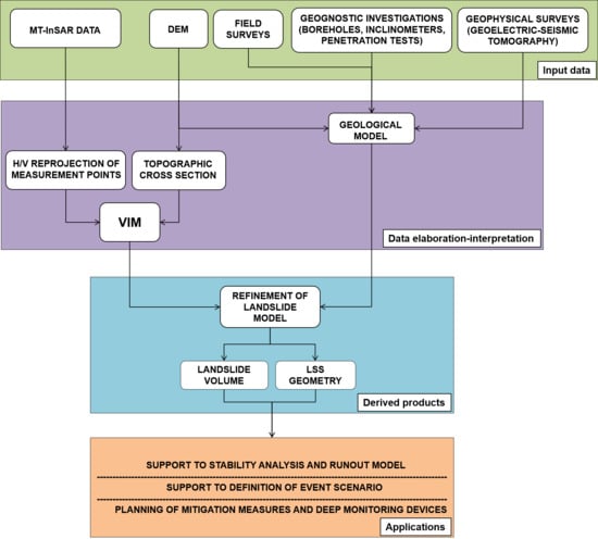
2. Materials and Methods

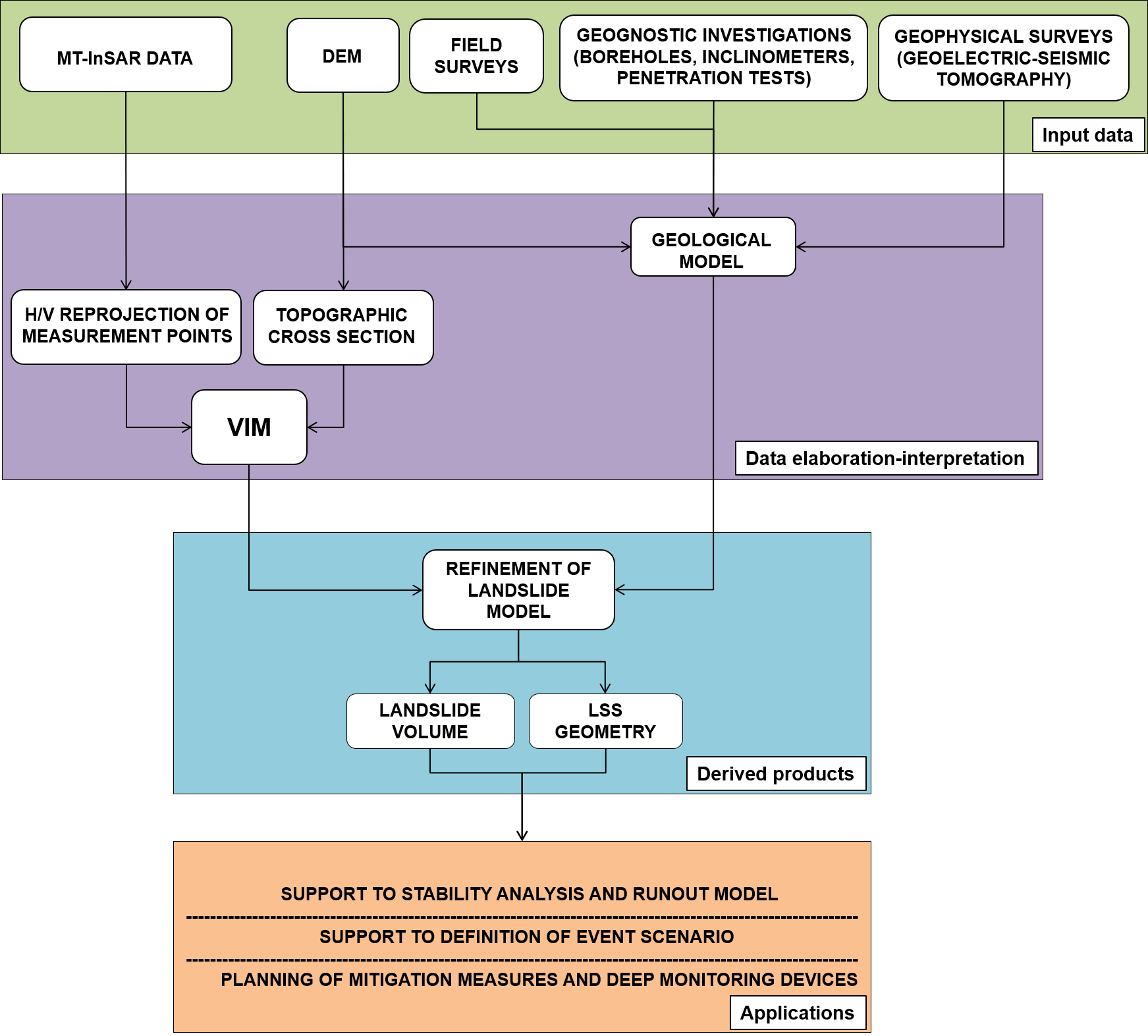
2.1. The Vector Inclination Method

The method proposed by [31]—here named the vector inclination method (VIM)—starts with the assumption that (i) a point on the surface of a sliding soil or rock mass will move in a direction that is parallel to the slope of the sliding surface beneath, provided (ii) the mass moves as a rigid body. A third assumption is that (iii) a single sliding surface exists. This means that theoretically VIM has a limited or null applicability to flow-type landslides where the movement vectors vary with depth and the superficial displacement does not exactly reflect the movements on the basal plane. To use this method a displacement monitoring must be implemented and measurement points (MPs), taken along a cross-section of choice, must be available. Then, the method consists of (see Figure 1a):

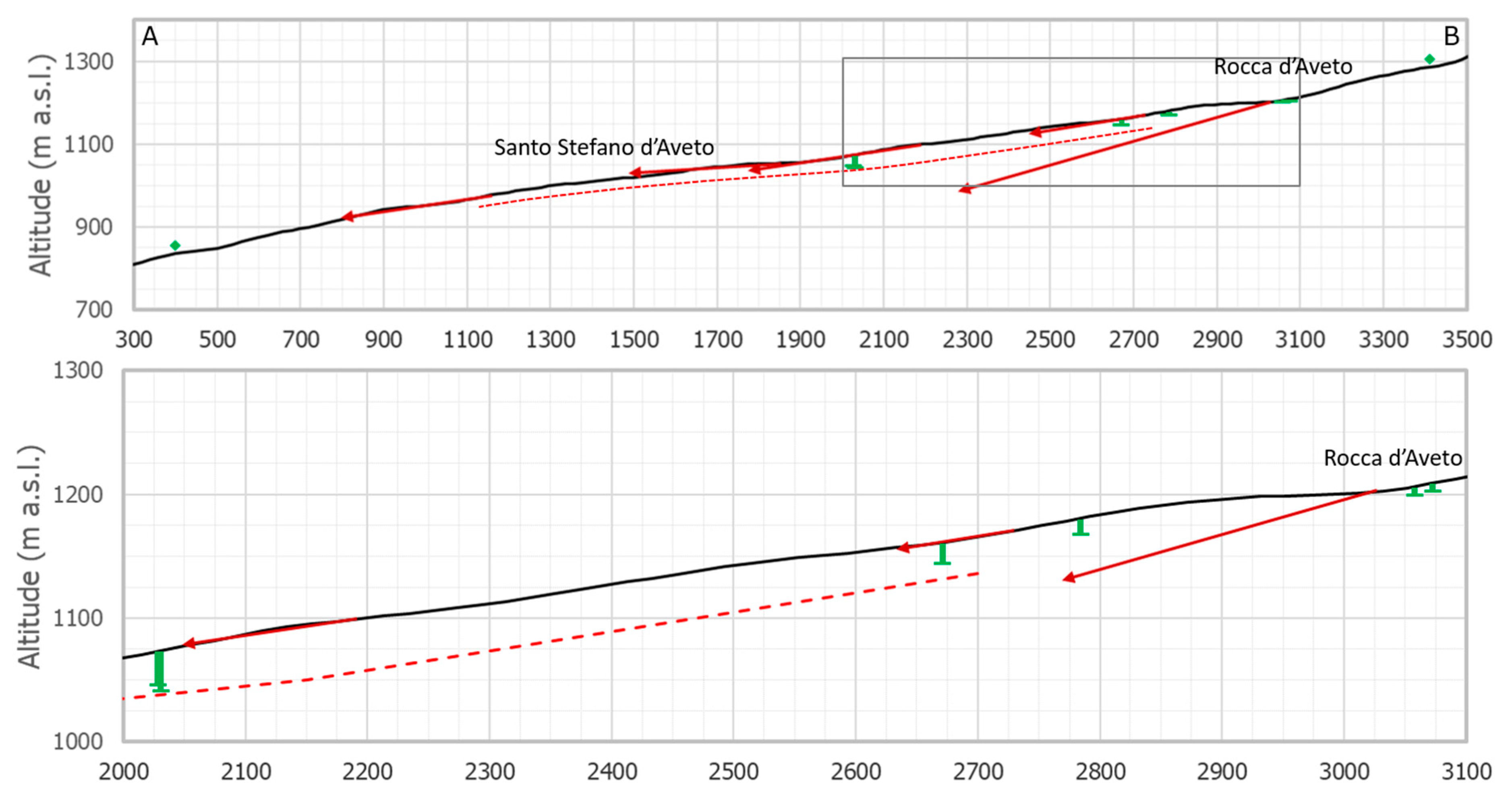
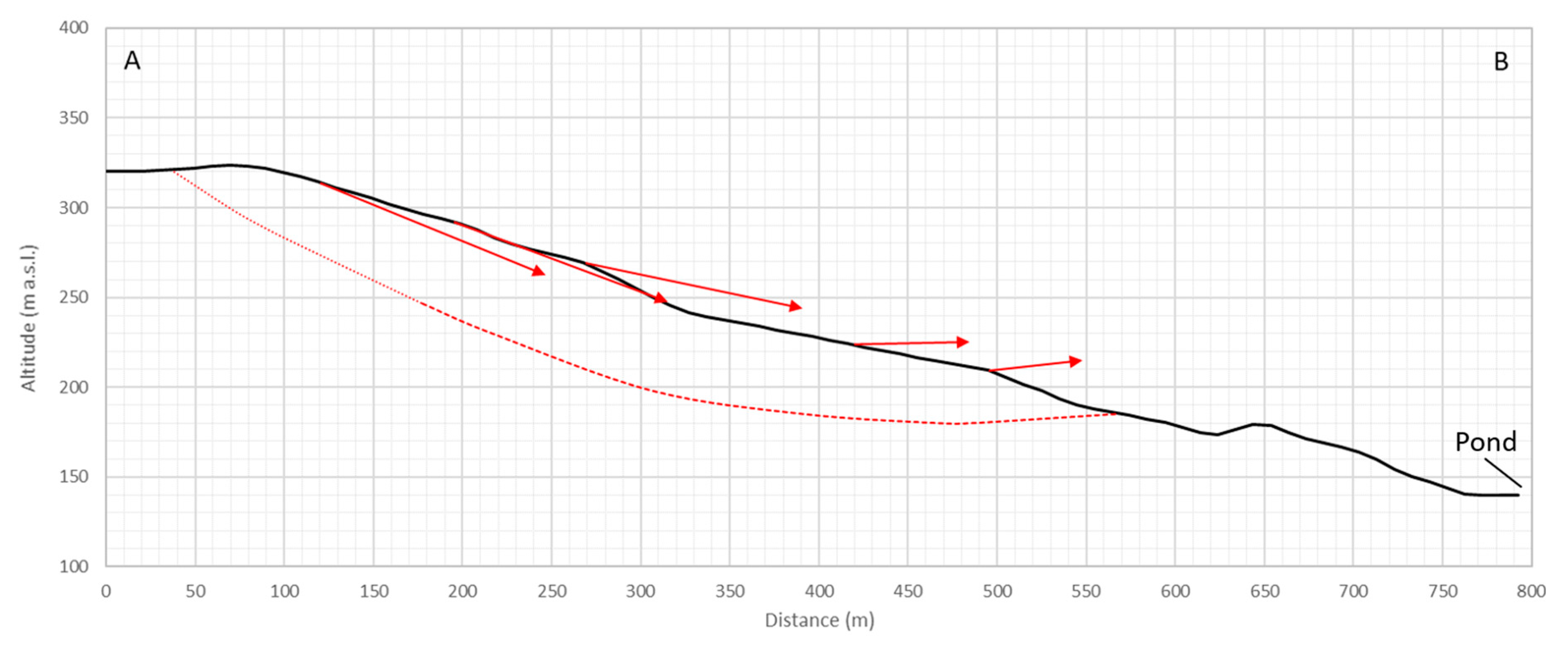
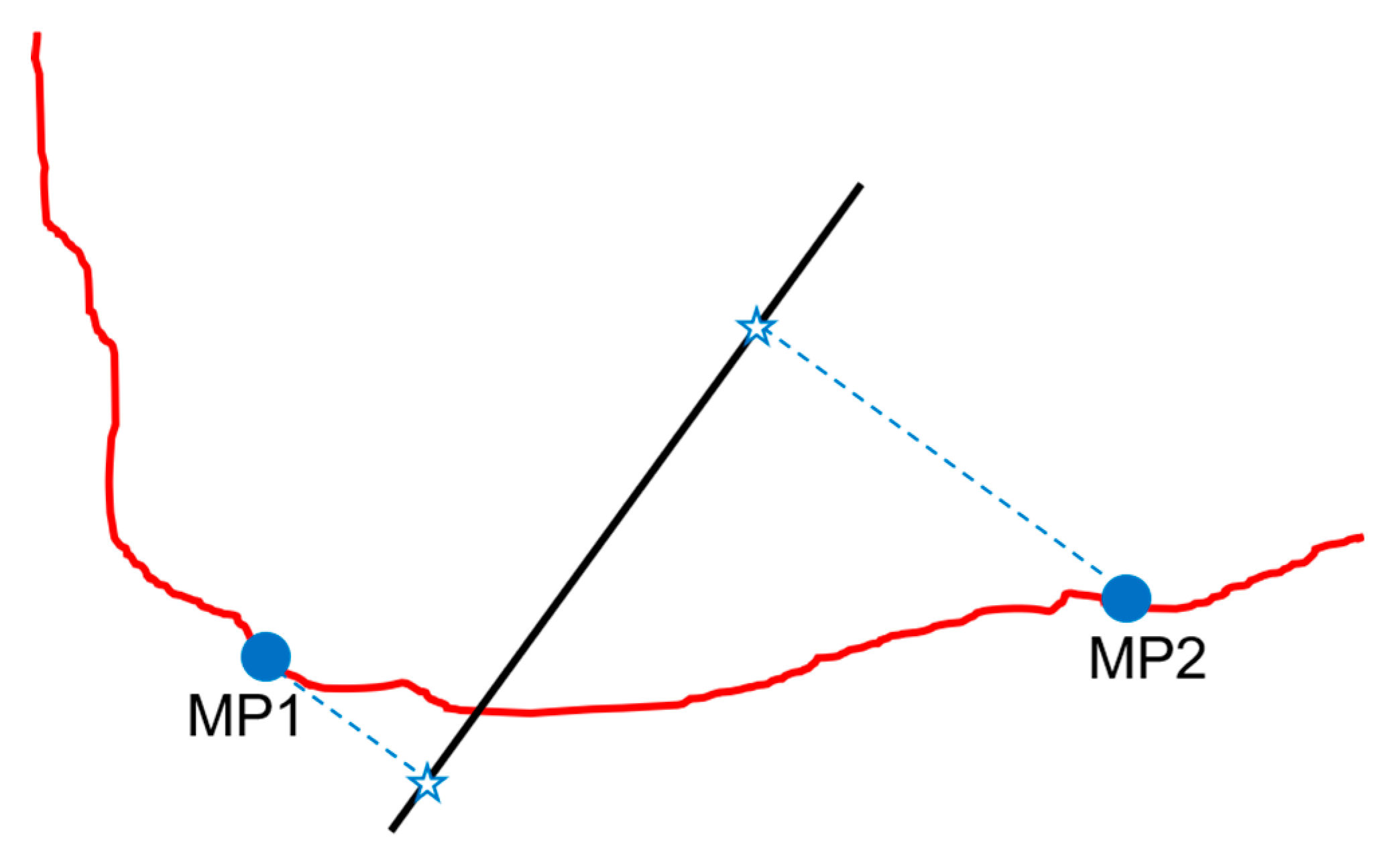
• drawing the cross-section of the landslide intersecting the MPs and marking with arrows the vectors of movement (V_i) measured at each point; note that the first vector should be representative of the movement close to the main scarp.
• drawing the normals to each vector and finding the intersections between two consecutive normals (O_i);
• drawing the bisection lines between two consecutive normals (blue dotted line in Figure 1a);
• drawing a line parallel to the first movement vector (V₁), beginning from the back scarp and ending at the intersection with the first bisection line, and finding P₁, which represent the first point of the sliding surface.
• a second line, parallel to the second vector (V₂) is drawn from P₁ to P₂. This procedure is repeated for each movement vector;
• the whole procedure is then repeated starting from the toe and working upslope to find a second sliding surface to be interpolated with the first one.

In [32], an alternative graphical solution, which provides the same results but with circular interpolation, was suggested (Figure 1b). The first two steps of the procedure are the same as above but, instead of drawing the bisection line, a circle is centered on O1 and drawn passing through P1 (blue dotted circle in Figure 1b); then, a second circle, centered on O2 and passing through P2 is drawn (magenta dotted circle in Figure 1b) and so on, for every MP, until the LSS is obtained (red curve in Figure 1b).

Since it is a graphical method, there is no way to precisely compute the margin of variability due to error, which is mostly due to graphical limitations and, ultimately, to the scale. Therefore, we can estimate a vertical error bar on the location of the LSS as less than 1% of the total length of the landslide section. The trueness of the LSS, that is, the divergence between the real and the calculated LSS, is impossible to calculate because it can vary along the body of the landslide, and depends on the quality and representativeness of the monitoring data (and not only by VIM). Furthermore, eventually, because the real LSS is unknown, it is, at best, the result of a reconstruction, the accuracy of which is often undetermined.

In the following section we applied this approach to a number of landslides. Since the inclination of the vectors is crucial, we have been careful to maintain a 1:1 ratio between vertical and horizontal distance when calculating the LSS on the different cross sections (or else the vectors inclinations should be modified accordingly). As this method is completely graphical, the slope profiles and the movement vectors are the only data required to reproduce our results.

2.2. Satellite Interferometry

The proposed methodology begins with the generation of a deformation map for the selected landslide areas. The ground deformation maps are derived by analyzing large stacks of SAR (Synthetic Aperture Radar) satellites images by means of differential radar interferometry, a well-established remote sensing technique that exploits the phase shift of the back-scattered electromagnetic signal between two or more coregistered images, acquired over the same target area. The returning phase values contain a number of terms, among which are contributions related to displacement, decorrelation, stereoscopic effects, and atmospheric artefacts. The main idea behind any interferometric approach is based on isolating the phase term that is actually related to a variation of the sensor-to-ground path length.

Over the study areas, ESA (European Space Agency) C-band ERS, Envisat and Sentinel-1 (center frequency 5.4 GHz, wavelength 5.6 cm) satellite data in ascending and descending geometries were acquired and processed using different multi-interferometric approaches, in order to obtain comprehensive views of the deformation field of the landslides and to make it possible to infer key features concerning its mechanism and behavior. Historical ERS (1992–2000) and recent Envisat (2003–2010) datasets have been processed in the framework of the Special Plan of Remote Sensing of the Environment (Piano Straordinario di Telerilevamento Ambientale, PST-A). This project, led by the Italian Ministry of the Environment, was aimed at creating a set of layers, among which is a database of ground deformation measurements over Italy by means of multi-interferometric processing [37], to assess the stability evolution of the territory. ERS and Envisat images, acquired every 35 days with an incidence angle of 23° and with a ground resolution of 25 × 5 m, were processed using the PSP (Persistent Scatterer Pairs) [38], PSInSAR [39], and SqueeSAR [40] approaches, some of the most advanced techniques specifically implemented for the processing of multitemporal radar imagery. The current Sentinel-1 constellation (2014) operates in the TOPS (Terrain Observation with Progressive Scans; [41]) imaging mode with an incidence angle ranging from 36° to 40°. Developed within the Copernicus initiative, the Sentinel-1 mission [42] is a constellation of two twin satellites, Sentinel-1A and Sentinel-1B. Launched in April 2014 and in April 2016, respectively, they share the same orbital plane and offer an effective revisiting time of six days (12 days for each single sensor), which is extremely suitable for interferometric applications. With respect to previous SAR satellites: Sentinel-1 data exhibit some favorable characteristics: regional-scale mapping capability, systematic and regular SAR observations and rapid product delivery. Interferometric wide-swath Sentinel-1 images, featuring a spatial resolution of 4 × 14 m, were processed by means of the SqueeSAR algorithm.

The PSInSAR approach [39] is the first method implemented for the processing of temporal series of coregistered SAR images acquired over the same target area. The main idea behind PSInSAR is to identify point-like targets, PS (Permanent Scatterers). PS are radar-bright, point-like targets with a dominant signal-to-noise ratio within the radar image, such as pixels corresponding to man-made objects, outcropping rocks, debris areas or buildings, which register a stable radar signal across the whole interferometric stack. The PSP algorithm [38] is based on the identification and analysis of PS working only with pairs of points (“arcs”). By comparing the SAR signal at a given point only with the signal in other points close to it, the PSP approach makes the method insensitive to any spatially correlated signals, such as atmospheric or orbit phase contributions. PSP is able to identify PS in natural terrain and PS characterized by non-linear movements. The SqueeSAR [40] approach, a second-generation PSInSAR algorithm, allows for the identification of both point-wise coherent scatterers (i.e., PS) and partially coherent Distributed Scatterers (DS). DS are statistically homogeneous groups of pixels sharing similar reflectivity. DS correspond to homogeneous ground surfaces, such as bare soil, deserts, debris-covered slopes and scattered outcrops. Through multi-interferometric approaches (Multi-temporal Interferometric Synthetic Aperture Radar, MT-InSAR), the LOS (Line Of Sight) deformation rate can be estimated with an accuracy theoretically lower than 0.1 mm/y, at least for very stable PS over a long-time span [43]. PSI analysis is designed to generate time-series of ground deformations for individual reflectors. The accuracy of a single measurement in correspondence to each SAR acquisition ranges from 1 to 3 mm [43]. Displacements are calculated relative to a stable PS within the frame and to a unique reference image.

InSAR-based displacements are one-dimensional measurements and, so, the resulting datasets can estimate only a percentage of the three-dimensional real motion of a landslide (i.e., the component corresponding to the projection along the satellite LOS). Under the assumption of absence of N-S deformation components, the availability of two different orbits of acquisition gives the opportunity to calculate the E-W and vertical components of the true movement vector.

A procedure to decompose satellite InSAR data has been described in [44,45]. The entire dataset is resampled into grids (with cell size generally ranging from 75 × 75 m to 50 × 50 m). Within each cell, the averaged ascending (V_A) and averaged descending (V_D) velocities are combined to derive the vertical (V_V) and East-West (V_E) ground velocity components, by solving the following formulas (Equation (3)):

$$\begin{array}{c}{\mathrm{V}}_{\mathrm{A}}={\mathrm{V}}_{\mathrm{V}}\cos (-{\mathsf{\theta }}_{\mathrm{A}})+{\mathrm{V}}_{\mathrm{E}}\sin (-{\mathsf{\theta }}_{\mathrm{A}}),\\ {\mathrm{V}}_{\mathrm{D}}={\mathrm{V}}_{\mathrm{V}}\cos {\mathsf{\theta }}_{\mathrm{D}}+{\mathrm{V}}_{\mathrm{E}}\sin {\mathsf{\theta }}_{\mathrm{D}},\end{array}$$

(3)

where θ_A is the LOS incidence angle in ascending orbit and θ_D the LOS incidence angle in descending orbit.

In this paper, we use the vertical and horizontal displacement vectors measured from the satellite to apply VIM. The cross-sections were selected to be possibly aligned with the direction of the expected movement (i.e., the steepest slope) and, at the same time, to intercept the highest number of MPs. This means that, in general, the cross-section is not aligned E-W (as with the movement vectors); therefore, the E-W movement vectors were reprojected along the cross-section, considering that the maximum movement is expected along the steepest slope direction. It is useful to remember the first assumption made in Section 2.1, i.e., the mass will move in a direction that is parallel to the slope of the sliding surface beneath; in fact, since the horizontal movements are reprojected along the cross-section where the maximum movement is expected, if a landslide experiences radial movements (i.e., the sides of a landslide diverge from the coaxial displacement either because they spread laterally or are dragged towards the central section, such as in [46,47], respectively), when these will be reprojected along the coaxial cross-section, their horizontal component will be underestimated with respect to the vertical one.

3. Results

VIM was tested on four landslides in Italy, characterized by different types of movement, material, size and kinematics. The selection of the case studies was accomplished by considering the following criteria:

• Good distribution of measurements: the top, middle and bottom sections of the landslide must be represented by at least one MP each. This criterion also implies that the available data were of good quality, in terms of accuracy.
• Satellite coverage in both geometries: in addition to the criterion above, both geometries are needed in order to derive the vertical and horizontal movement components.
• Different landslide characteristics: the landslides used were different in geological, geomorphological and geometrical terms. In particular, we wanted to stress test VIM on both rotational and translational landslides, with different depths and oriented along different azimuth angles with respect to the satellite LOS.
• Availability of validation tools: to evaluate the effectiveness of the method, independent sources (inclinometers, geological models) of the depth of the LSS were adopted.
• Different satellites: the method was tested using ERS, ENVISAT, and Sentinel-1 data, in order to see whether there were limitations or advantages depending on the satellites used.

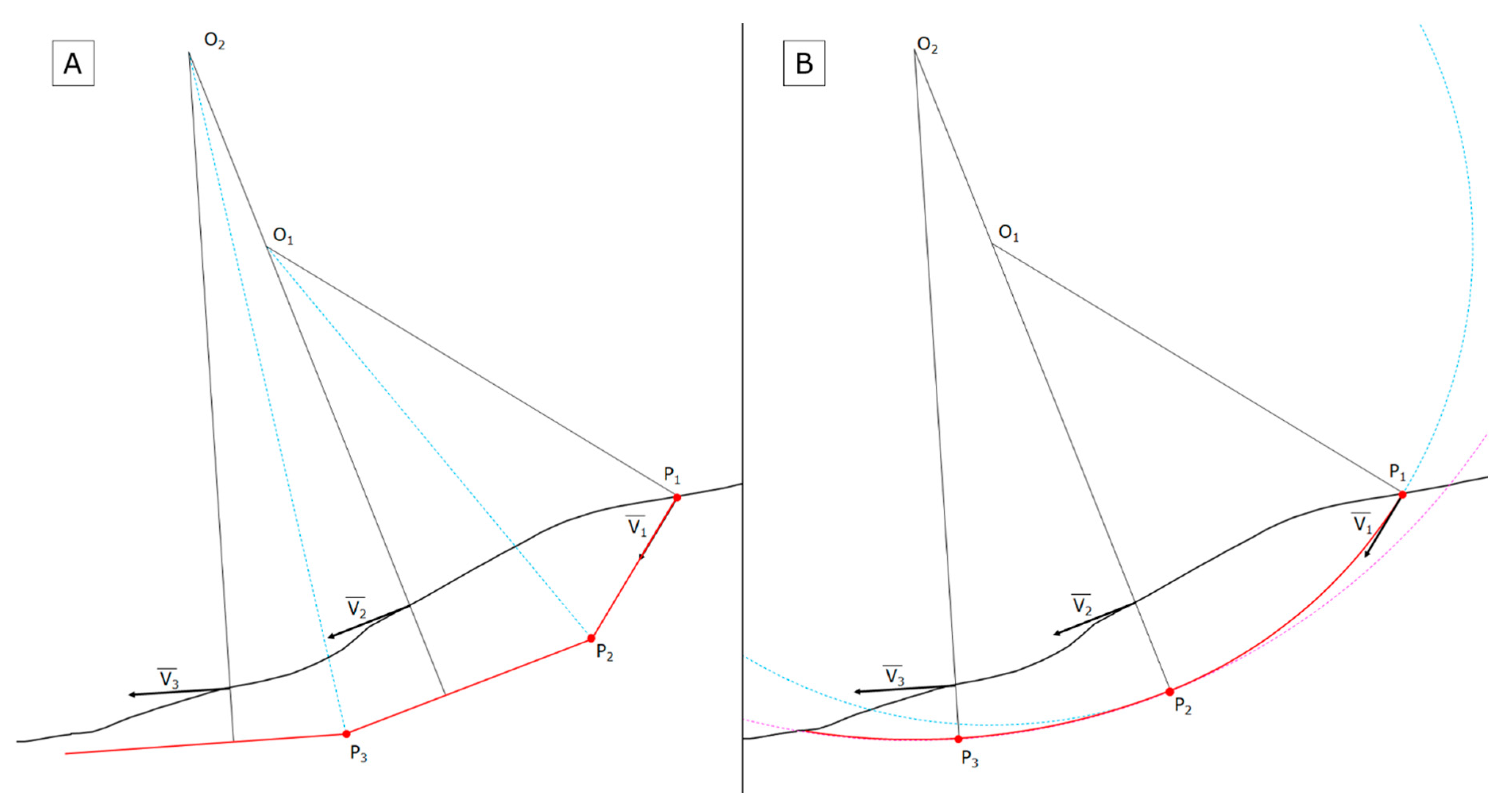
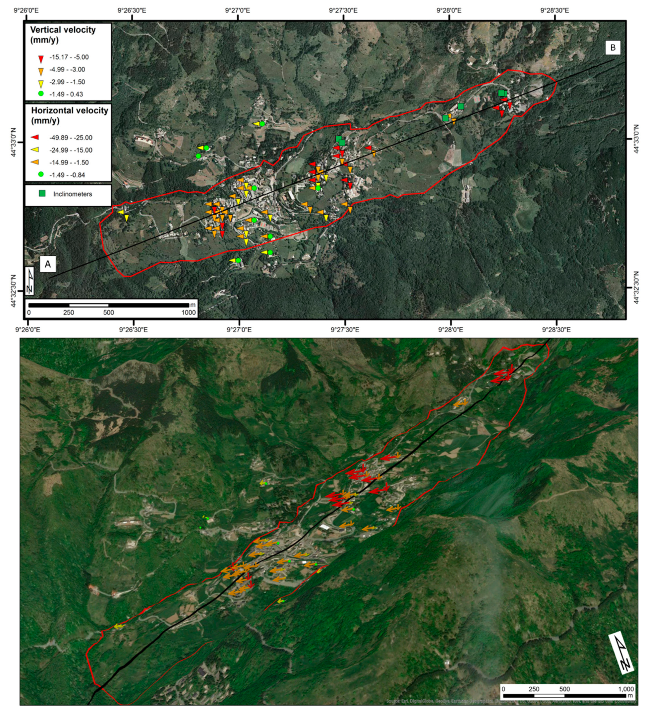
3.1. Santo Stefano d’Aveto Landslide

3.1.1. Santo Stefano d’Aveto General Description

The Santo Stefano d’Aveto landslide is located in the NE sector of the Genova province (Liguria region, northern Italy), in the Ligurian Apennine (Figure 2a). The landslide mainly involves unsorted glacial deposits, constituted of sandstone and ophiolitic clasts in a sandy-silty matrix, while the bedrock is constituted by the Ligurian Units, comprising a limestone, marls, sandstone and ophiolitic rocks [48].

This landslide is a complex slide-earth flow evolving from a height of about 1300 m a.s.l., where the main scarps are located, to about 825 m a.s.l. at the confluence of two small rivulets (the Rio Grosso and the Rio Freddo), which binds both the landslide flanks. The landslide body has an elongated shape, its main axis trends W-SW, with maximum length and width of 3.1 km and 600 m, respectively, and it has a total aerial extension of 1.3 km² and an estimated volume of around 10⁷ m³ [49]. The landslide cover consists of annual and permanent crops, deciduous and mixed forests and small urbanized areas—the village of Santo Stefano d’Aveto and the two small hamlets of Roncolungo and Rocca d’Aveto (Figure 2b,c). The landslide, which is extremely slow, has been classified as active in the uppermost sector and dormant in the lowermost, where the main part of the inhabited areas are located (Figure 2b); therefore, its effects are only related to moderate building damage. In fact, the buildings and the main roads have been extensively affected by cracks and damage and are often subject to repair and consolidation works. Six inclinometers and eleven piezometers have been installed inside the landslide perimeter, which took place during a geotechnical campaign carried out from 2000 to 2006 ([44]; Figure 2b,c).

3.1.2. Santo Stefano d’Aveto LSS Results

The sliding surface of the Santo Stefano d’Aveto landslide [44] has been inferred using ERS satellite data ranging from 16 May 1992 to 19 December 2000 (Figure 3). The distribution of MPs is not uniform as they are clustered in the central part of the landslide (where buildings are more numerous). Six inclinometers are installed in the top half of the landslide, which were used for validation (green dashes in Figure 4). The uphill two record the depth of the LSS respectively at 8.5 and 9 m, the two in the middle at 17 and 18.5 and the lowest two at 22.5 and 12.5 m (green dashes in Figure 4). This suggests the presence of a gradually deepening surface, which reaches its maximum depth (of around 20 m) not close to the crown but at one fourth of its total length.

Reconstruction performed using VIM suffers from a lack of MPs at the lower and upper bounds of the landslide and, so, the LSS was drawn only in the central part, using the MP uphill as the starting point (Figure 4). The vectors were approximately parallel to the slope, producing a planar surface the geometry of which is robustly based on data that are consistent with each other, showing all similar inclination values (red arrows in Figure 4). If interferometric data near the toe were available, these would be expected to become horizontal. The depth obtained from VIM was in good accordance with the in situ measurements (green dashes in Figure 4); furthermore, in order to intersect more MPs, the LSS was computed along the major axis of the landslide (where the maximum depth is expected), while the inclinometers were closer to the right boundary (where the landslide is expected to be shallower). It must also be noted that the two westernmost inclinometers are only 31.5 m afar but record a vertical difference of the LSS of 10 m, which gives an idea of the lateral variability of this landslide’s LSS.

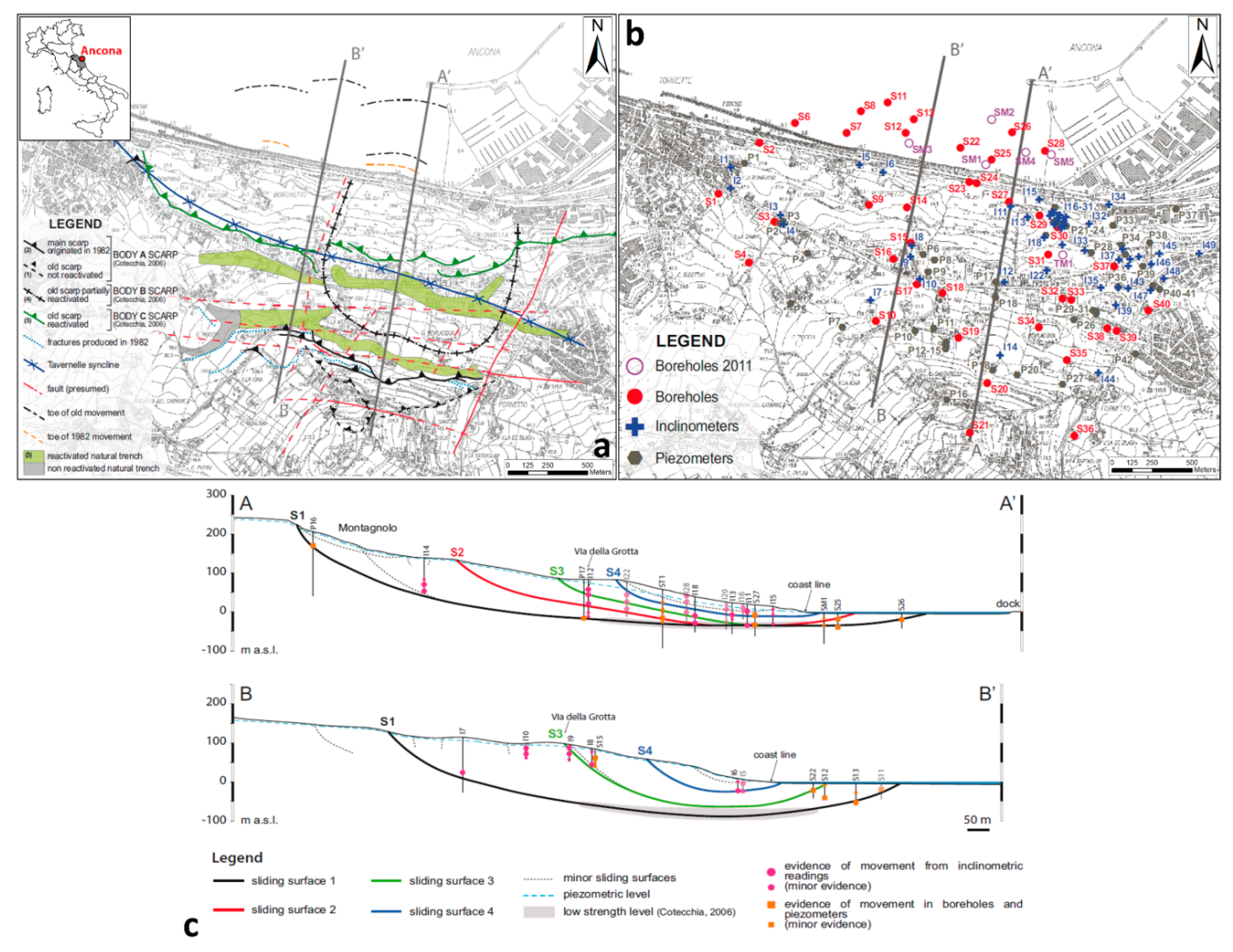
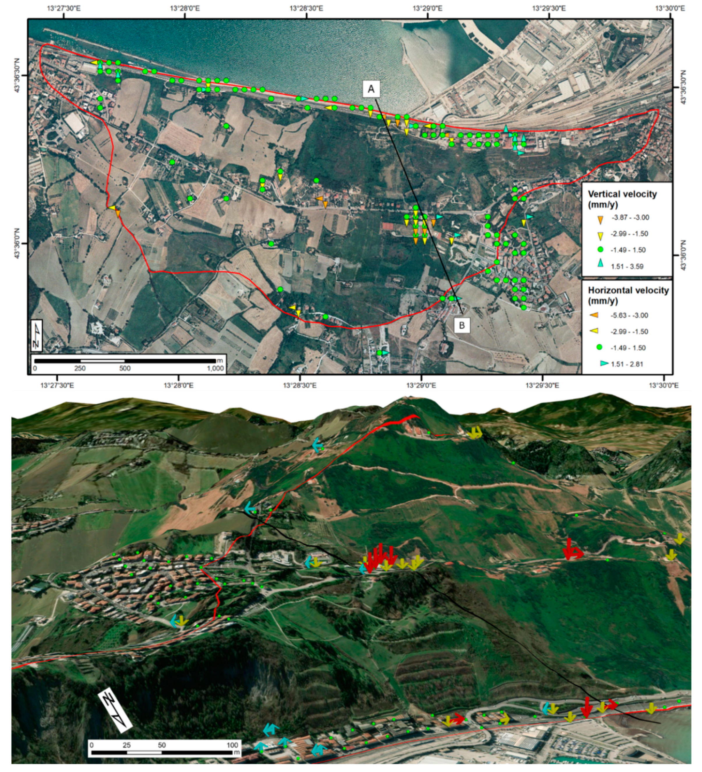
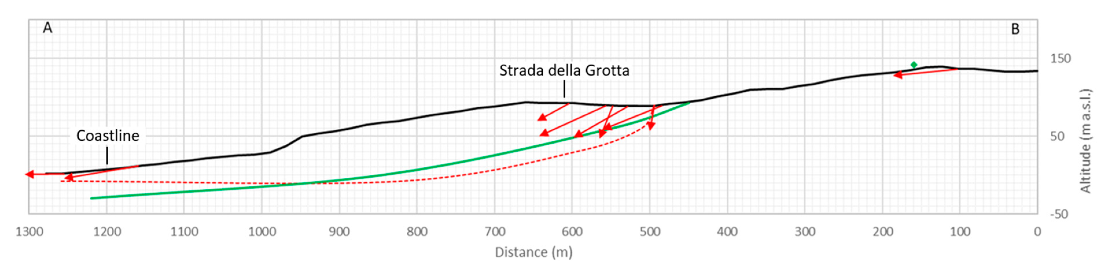
3.2. Ancona Landslide

3.2.1. Ancona Landslide General Description

The study area is located along the central Adriatic coastal area to the west of the city of Ancona (Marche region, central Italy; Figure 5a). The main recent reactivation of the landslide occurred on the N slope on the Montagnolo hill, an area historically affected by slope instabilities, on 13 December 1982. This event had an area of more than 3.4 km², which began near the top of the hill (at 170 m above sea level) reaching a maximum width of approximately 2 km near the coastline, and involved about 1.8 × 10⁸ m³ of material [50,51]. The landslide involved marly clay with thin sandy and silty interlayers, and a diffused eluvio-colluvial deposit cover [52].

The main direction of displacement was roughly S to N and it damaged or destroyed almost 280 buildings, involving the railway and the roads that run along the coast. Since 1983, monitoring instruments such as piezometers and inclinometers have been installed, and topographic leveling, geophysical investigations [53], and numerical and analytical modeling have been carried out (Figure 5b,c). These studies enabled a conceptual scheme of the landslide (Figure 5b), characterized by three main bodies showing rotational-translational movements: (i) body A, which is very deep and with very large areal dimensions, is defined by the upper scarps at the hilltop and was characterized by rather limited movements during the 1982 event; (ii) body B, superimposed on body A, involves the central part of the slope, which underwent more intense deformations during the 1982 event; and (iii) body C, delimited by the lower long scarp, which was partly reactivated in 1982 [51]. The sliding surfaces of the main landslides emerge offshore, at a maximum distance from the coastline of over 250 m (Figure 5c). The landslide features (extent of the area, the simultaneous occurrence of deformations, the presence of trenches, very old onset of movements, step-wise evolution, and independence of the movement from the surface morphology) indicate that the main movement of the studied landslide was deep-seated, probably at more than 100 m depth [54]. Therefore, the Ancona landslide can be defined as a deep-seated, multiple, compound (rotational–translational movement), and recurrent (slow, continuous movement with short and sudden accelerations) landslide. Considering the superficial flow and slide type landslides, the whole phenomenon can also be considered as a composite mass movement [51].

3.2.2. Ancona LSS Results

The data set used in this case consisted of ENVISAT data acquired between 15 December 2002 and 14 July 2010 (Figure 6). The density of MPs in both geometries, required for the vertical and horizontal composition, is high along the coast and in the SE part of the landslide, in an urbanized area. Therefore, the profile was drawn such that it crossed this area while being as aligned as possible to the direction of movement (roughly S-N) and to the geological profiles available (in particular to the profile AA’, in Figure 5).

The main cluster of MPs is located at the mid-upper part of the landslide. Here, two MPs on the W side of the cluster have a dip of 68°–80°. This steep immersion suggests the presence of the crown of a secondary LSS. The remaining MPs in this zone have a dip ranging from 22° to 30°, indicating the average inclination of the surface in this area. The two terminal MPs are almost horizontal toward the coastline (10° and less than 1°, respectively) (Figure 7). The complete absence of points in between prevents us from determining where the LSS begins to horizontalize, which influences volume estimations, therefore, in this case, the two inclinations were interpolated linearly such that the change of inclination roughly occurs midway.

Comparison with the profile AA’ reconstructed by [51] (Figure 5c) provides an interesting validation (Figure 7). In particular, the surface called S2 (relative to body B mentioned in Section 3.2.1) starts at the same location of the MP cluster, confirming that the steep displacement vectors can be related to this movement, although satellite data suggest a steeper crown. The two profiles have a comparable geometry. The profile reconstructed by [51] continues beyond the coastline (Figure 5c), while using radar interferometry, it is impossible to retrieve displacement information in the underwater sector of the landslide.

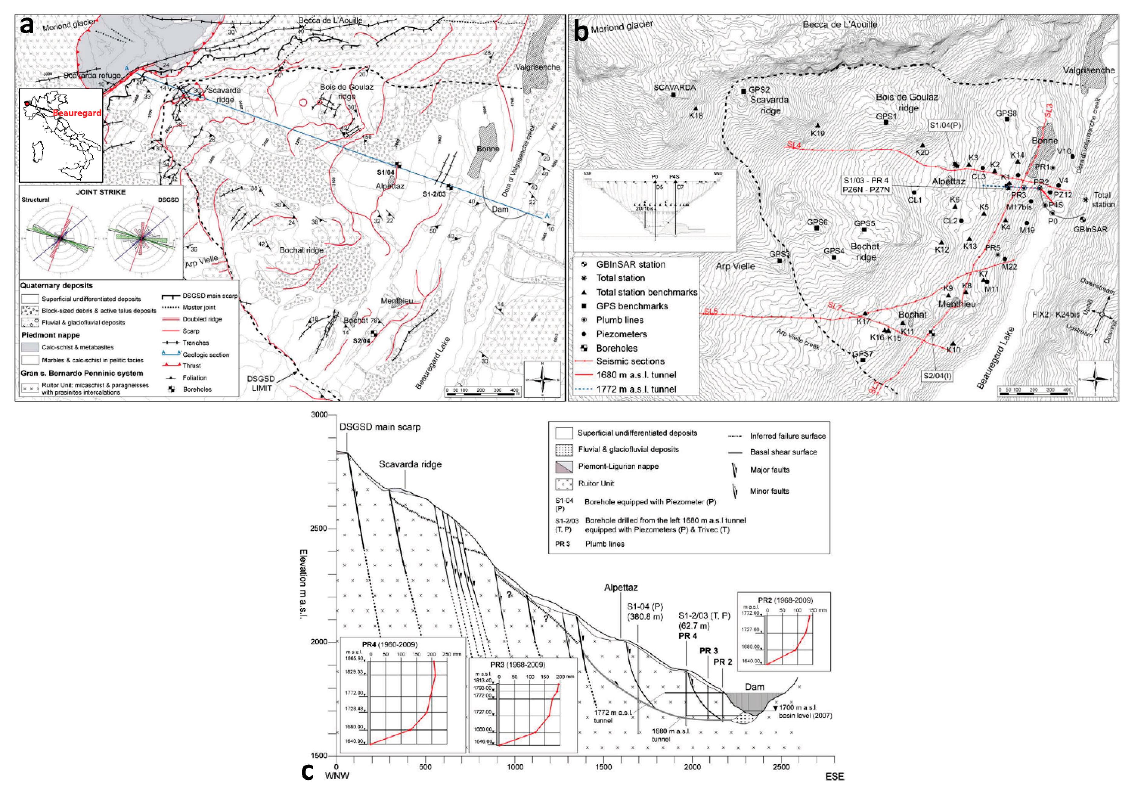
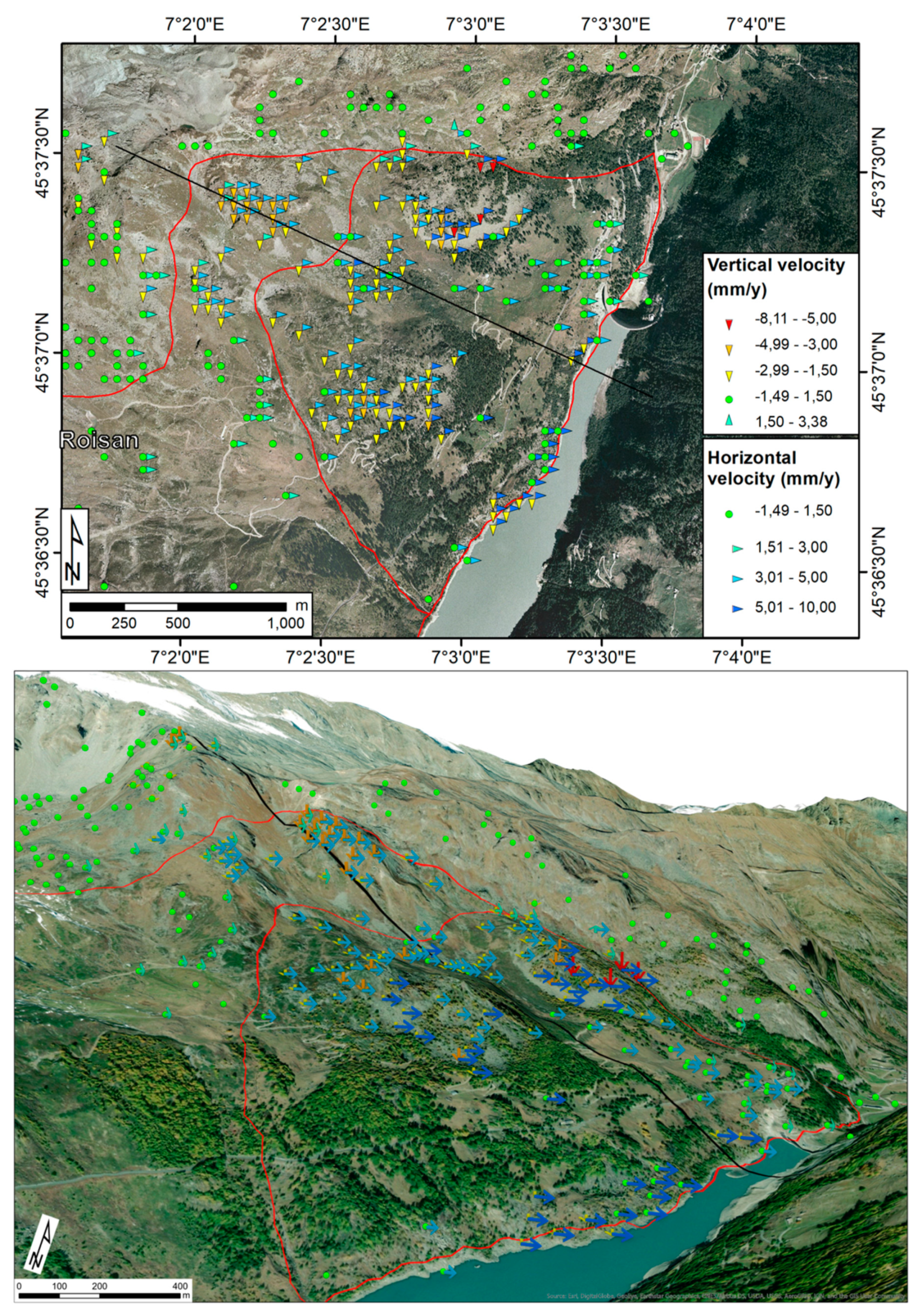
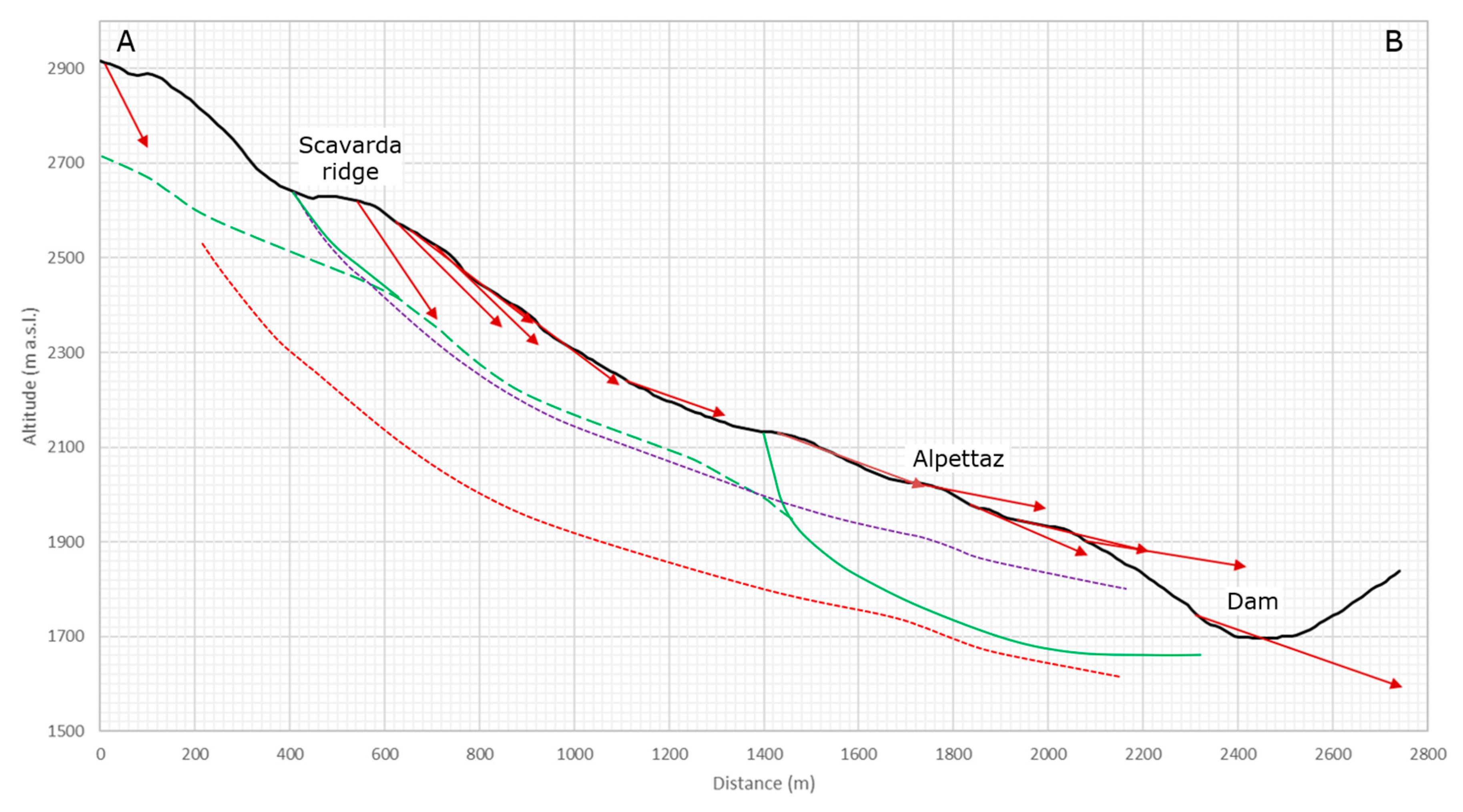
3.3. Beauregard Landslide

3.3.1. General Description

This landslide is located in the Aosta Valley (on the Dora di Valgrisenche river), in the Western Italian Alps (close to the Italian–French border) in NW Italy (Figure 8a). The phenomenon is an extremely slow-moving, deep-seated gravitational slope deformation (DSGSD) affecting the left slope of the valley and impinging on a 132 m-high concrete arch-gravity dam [55]. The metamorphic rocks cropping out all along the Valgrisenche valley belong to the Pre-Permian crystalline basement of the Ruitor Unit, which consists of predominant garnet micaschists and albite-bearing paragneiss with abundant intercalation of metabasites [56]. The basal portion of the left slope overlays a deep pocket of glaciofluvial sediments, which were completely replaced by concrete to a depth of 200 m into the left slope during the construction of the dam ([57]; Figure 8b). The presence of extended rock slices of the Ruitor Unit directly overlaying the remaining fluvio-glacial deposits is clear evidence that, after glacial debutressing, the valley left slope toe has slipped down.

Considering the geomorphologic and morphotectonic features, the deformation zone involves a significant portion of the slope and extends approximately 1500 m in height from the toe (1700 m a.s.l.) to the mountain ridge (3200 m a.s.l.), with a maximum of 2.3 km in length and a 1.9 km in width [55]. Its maximum thickness has been estimated to be 260 m [58]. The double ridge of Becca de L’Aouille Mt., interpreted as the main scarp delimiting the DSGSD surface of the rupture, bounds the N sector, trending E–W with a maximum relief of about 250 m. By the Scavarda Refuge the scarp turns to the S, forming a wide niche from which a rocky ridge (Scavarda ridge) has been lowered. In the upper part of the ridge (i.e., above the main DSGSD scarp), a swarm of trenches up to 3 m wide trending parallel to the valley is present. In the middle and lower portions of the landslide slope, it is possible to distinguish two ridges, one to the N (Bois De Goulaz) and one to the S (Bochat), characterized by bulging and convex profile. In the central slope sector, between 2000–2200 m a.s.l., one major concave scarp is present. At lower elevations (1800–2000 m a.s.l.), close to the reservoir, numerous minor linear scarps and counterscarps trending parallel to the valley axis can be recognized. Geological, hydrogeological and geotechnical investigations have underlined the presence of a deep-seated shear zone in the central lower sector (over 20 m and 8 m in correspondence to boreholes S1-04 and S1-03, respectively), while a third borehole in the lowermost southern sector highlighted a major shear zone at 147 m depth (Figure 8b,c). The slope movement is correlated to the dam response and has caused a state of damage in the structure. The occurrence of a nonhomogeneous surface displacement pattern across the Beauregard landslide, with larger displacements (35–40 mm/year) for the upper slope (Scavarda ridge) and small and steady displacements (10 mm/year) at the landslide toe, suggests two landslide sectors with different kinematic behaviors [55].

3.3.2. Beauregard LSS Results

Sentinel-1data processed with SqueeSAR algorithm [40] and spanning from 10 October 2014 to 7 March 2019 were employed for the Beauregard landslide, which has a good coverage of MPs (Figure 9). To validate the information about the depth and geometry of the LSS, the study provided by [59] was used. In [59], a cross-section of the landslide is provided, which was partly derived from two boreholes (visible in 4b and 4c) drilled in the bottom part (solid green line in Figure 10, at the toe bottom of the landslide) and partly interpreted from seismic surveys (dashed green line in Figure 10, at the middle and top part of the landslide). Notably, whereas the bottom part reaches a maximum depth of around 240 m, the part interpreted by geophysical surveys is shallower (from 100 to 200 m deep), resulting in an uncommon geometry. The trace of the cross-section proposed by [59] is shown in Figure 8a.

The Scavarda ridge was interpreted by [59], as the day-lite portion of the main DSGSD surface (also represented as a solid green line in Figure 10). At the same time, seismic surveys indicate a prosecution of the landslide uphill of the ridge. The presence of movements above the presumed landslide scarp was confirmed by interferometric data (Figure 9). Notably, according to [59] and possibly based on a geomorphological interpretation, the LSS progressively deepens quite suddenly between 1400 and 1600 m. The few interferometric MPs in this area do not indicate such variation of inclination; however, the lower density of points does not allow for conclusive results. Other minor scarps were included in the cross-section by [59], probably hypothesized based on slope changes of the topographic surface, which are not considered as relevant in this case. Given the uncertainty related to where the movement begins, two inversions using VIM were done, one assuming that the landslide starts at the Scavarda ridge (purple dotted line in Figure 10) and one assuming that it starts from the first MP showing a consistent displacement (red dotted line in Figure 10). As the interferometric data show a roughly constant inclination of the movement vectors, the calculated LSS did not result in any deepening towards the toe. Interestingly, the surface starting from Scavarda ridge fits the results provided by the seismic surveys very well. At the same time, the first vector at the left side in Figure 10 displayed a significant movement with a 63° of inclination, which cannot be dismissed. Calculating the LSS from here determines a good correspondence at the toe of the landslide, where VIM provides a 10% deeper result with respect to the surface obtained by [59]. As both calculated surfaces fit with one or another portion of the landslide, this may also suggest the possibility that two LSSs coexist in this case.

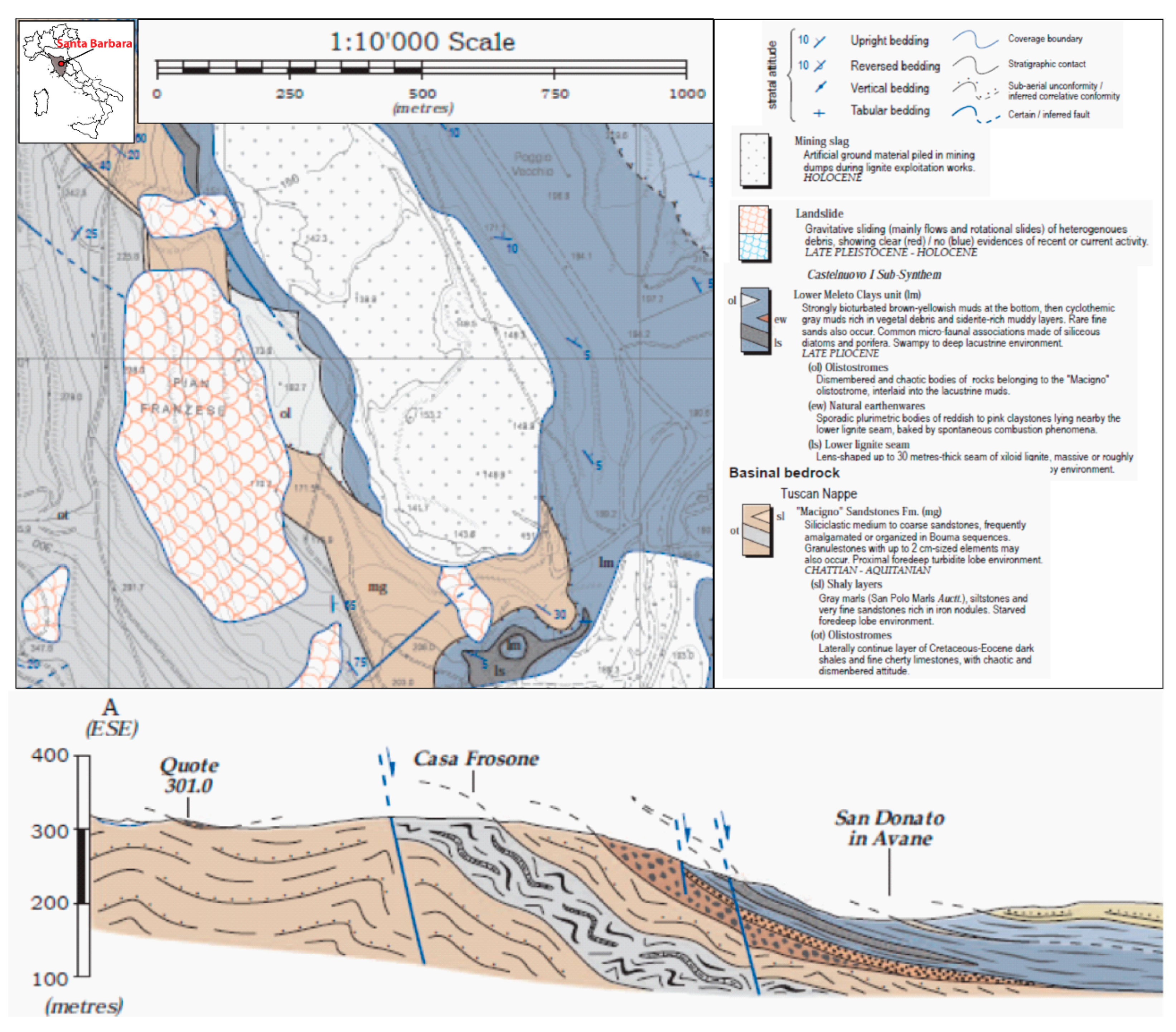
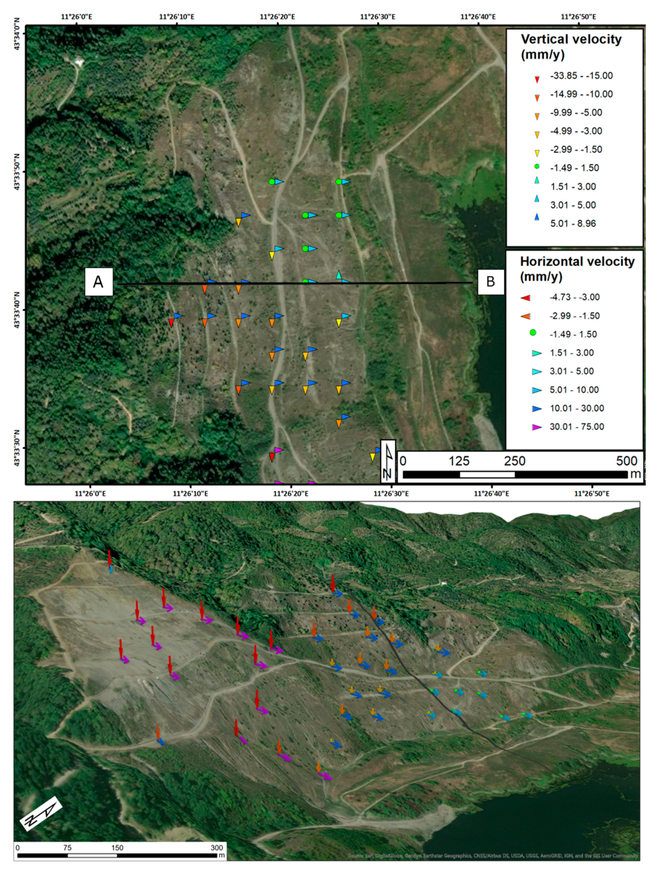
3.4. Santa Barbara Landslide

3.4.1. General Description

The Santa Barbara landslide is located in a small sub-basin (the Santa Barbara Basin) belonging to the Plio-Pleistocene Upper Valdarno Basin [60,61]. From a stratigraphic point of view, the basin bedrock is represented by turbidite sandstones, interbedded shaly olistostromes and locally gray marls (“Macigno” Sandstones Fm.; [62]) (Figure 11). In the study area the basin is filled with muds and lignite of the Lower Meleto Clay [63]. The Lower Meleto Clay unit has a maximum thickness of some 100 meters and has been related to a palustrine-to-lacustrine system, which is sporadically affected by gravitational basin borders collapses (olistostromes).

The landslide develops on a NW-facing slope in the “Pian Franzese” area. According to [63], an olistostrome of dismembered shale and limestone fragments, reaching in some boreholes up to 40 m in thickness, has been recognized (Figure 11). Mining slags cover the study area downslope with respect to Pian Franzese. From a structural point of view, the basin is represented by a gentle syncline dissected by normal faults. The basin sedimentary fill dips 5° to 10° towards E-NE (Figure 11).

3.4.2. Santa Barbara LSS Results

The data analyzed for Santa Barbara were from Sentinel-1 constellation, spanning from 12 October 2014 to 15 January 2020. This case study was chosen by giving priority to the criterion of having a good set of interferometric data even though no other validation information was available. Therefore, the result was evaluated according to the geological and geomorphological consistency of the determined shape of the LSS.

Data are well distributed along the slope but are absent at its foot. The inclination of the vectors gradually changes from 22° at the top, 10° in the middle and to almost horizontal (with a slight upward component) in the bottom part (Figure 12).

The shape of the LSS obtained is very regular and its depth depends on the point where its intersection with the ground surface is placed. The presence of an upward tract of the LSS is a strong indication that the toe is located nearby. Indications about the landslide’s boundaries can usually be retrieved by geomorphological evidence, however, in this case, the slope was heavily modeled by quarrying activities in a “bench and wall” fashion. The flat area at the foot of the slope is also affected by human intervention, with landfills and pits (now partially filled with water, as visible in Figure 12). The LSS was drawn at the foot of the slope considering the location of the bottom MP (Figure 13). The resulting landslide reaches a maximum thickness of 50 m and is consistent with the displacements of the at least 40 m-deep olistostrome occurring within the clays and dipping with low angles along the slope according to the geological information in [63].

4. Discussion

4.1. Case Studies

Each of the cases presented provides useful insight into the validity of VIM using satellite interferometric data. First of all, there was no apparent difference between the three types of satellites used (ERS, ENVISAT and Sentinel-1). Even though a higher resolution of a satellite sensor is linked to a higher MP density, the data coverage is also affected by other factors (such as land cover) and can be improved depending on the processing algorithm used. In general, the resolution of C-band satellites has been proved enough to achieve good results. For example, the ERS data used for the Santo Stefano d’Aveto landslide demonstrated the applicability of VIM to a translational slide; even without any previous knowledge of the LSS geometry, which may not be intuitive, considering that the method proposed by [32] is based on circular interpolations.

In the case of the Ancona landslide, using ENVISAT images, a reliable LSS was obtained despite some objective difficulties. First of all, the landslide movement is almost S-N oriented, while the decomposition of the ascending and descending displacement and their reprojection into vertical and horizontal (W-E) directions assumes the absence of S-N deformation (see Section 2.1). This means that only a small percentage of the actual movement was visible; however, it was sufficient to draw a LSS consistent with the boreholes and inclinometers data (Figure 7). This case was also particularly complex, owing to the coexistence of multiple LSSs, whereas [31] assumed a single surface. Figure 7 shows that, near the location of the crown, some MPs record very different angles. A possible explanation for this is that those movements represent lateral differences in the landslide (Figure 14). A complementary explanation is that this dual behavior could be the effect of two different LSSs. The verticality of the two MPs giving indication of the crown is so distinct that this information can be considered a data constraint to correct the original LSS and come up with a third, integrated, LSS which takes into account the VIM results for the upper part and the boreholes and inclinometers data for the bottom and submerged part.

In any case, since the result of VIM is in good accordance with the previous reconstruction of S2 sliding surface, the assumption made in [31] that this method cannot be applied in case of multiple LSS is somehow loosened. Given that MT-InSAR data are relative to superficial displacement they consider the cumulated effect of all the LSSs. Logically, if a specific surface (e.g., S2) is dominant, that is the deformation measured by satellites is mostly related to movement occurring along that surface, then VIM will produce an LSS very close to that surface. On the contrary, if two or more LSS are competing, we expect that the resulting geometry will be the weighted average between the most active surfaces. Therefore, the fact that for the Ancona landslide VIM provides a surface close to S2 gives us an additional information, that is S2 is the one where most of the deformation occurs. This outcome is confirmed in [50] who points out that the inclinometer that recorded the highest displacement during the 1982 reactivation is the one intercepting S2, while S1 barely reactivated and S3 and S4 exhibited small displacements.

An even more complex case was represented by the Beauregard landslide. Provided that the surface used as reference was affected by a certain degree of uncertainty (especially the tract interpreted from geophysical surveys, shown by the dashed green line in Figure 10), two different results were obtained with VIM, depending on where the LSS starting point was set. This proves that, while the geometry of the LSS was well constrained by movement data, its depth requires knowledge of the point (toe or crown) where the LSS emerges. In fact, [31] pointed out that the toe and backscarp of the slip must be known; then the LSS should be initiated from the first MP, under the assumption that it is located close to landslide boundaries. In reality this is not always the case and the LSS should not be completed and extrapolated up to the ground level if movement data are clustered only in the central part of the landslide (as was the case for the Santo Stefano d’Aveto landslide, Figure 4). In contrast, external information can be used to determine the points along the topographic profile where the LSS originated from, such as geomorphological features suggesting the presence of the crown (as done for the purple LSS of Beauregard, Figure 10) or the toe of the landslide (as done for the Santa Barbara case study, Figure 13). It is also possible that the displacement recorded by satellites on Beauregard landslide are simultaneously affected by multiple competing LSSs and movements occurring at different depths and therefore are not precisely relatable to a specific surface.

All the cases shown are in good agreement with the assumption that the mass must move as a rigid body. However, this does not mean that the LSS must be regular. In fact, VIM is able to reflect hummocks and irregularities in the LSS, as partially visible in the Beauregard case (Figure 10), as a result from vectors whose inclination does not monotonically decrease along the slope. Even landslides experiencing variation in duration and magnitude of motion along the body do not represent a problem, as VIM depends on the inclination of vectors, not on their modulus, so effects of seasonality or spatially heterogeneous accelerations do not hinder the results.

On the other hand, there would be issues in applying VIM to an earthflow. In this case, if the landslide exhibits intense internal deformation to the point that the amount of displacement varies with depth, this can be approximated as a translative landslide with many (infinite) LSSs distributed along the thickness of the moving mass. Even if, on the contrary, the basal surface is well defined and the mass exhibits a plug-flow deformation, the surface movement vectors would still be mostly parallel to the slope, with a consequent lack of movement vectors able to indicate the depth of the LSS, unless the earthflow initiates as rotational slide in the source area, from where the initial inclination of the LSS could be retrieved. For these reasons, VIM is not suitable for earthflows, for which other methods, such as the one used in [46] and based on a non-Newtonian viscous flow law or the one using Equation 2 and a Newtonian viscous flow model can be more proficiently applied [64].

4.2. Advantages and Limitations

Based on the aforementioned considerations, it is possible to infer some important requirements which determine the quality of the result, whenever an LSS is inferred using VIM exclusively. Such requirements influence the outcomes of the method, regardless of the monitoring technique is used (i.e., not only satellite interferometry):

• MP close to the landslide crown or toe: in absence of geomorphological information or other indications concerning the boundaries of the landslide, this is important for pointing out where the LSS emerges and helps to anchor the rest of the surface. In other words, if MPs are only clustered in the central part of a landslide, no indication of the extent of the landslide or of its behavior at the crown (which is typically where the inclination of the movement vectors is highest) is available, unless it comes from other sources (e.g., surveys).
• High density of MPs: VIM assumes a circular surface until the next MP corrects its shape and intersects it with a new arc. In the cases above this always resulted in compound or translative surfaces. At least in the areas where the LSS is more susceptible to changes in inclination (e.g., near the crown) it is important to have at least two MPs close to each other, such that changes in the LSS geometry can be immediately detected. When MPs are present only in the central part of a landslide, conclusions about the depth of the LSS must rely on assumptions or on external information (e.g., geomorphology, boreholes, etc.); however, its geometry will still be reliable as it is grounded on monitoring data.

Focusing on the application of MT-InSAR to VIM, the four cases reported in this paper demonstrate the potential and limitations of this approach. The limits can be summarized as follows:

• It is difficult to precisely attribute a MP to a portion of the ground, especially after they have been resampled to obtain the vertical and horizontal components. The data used represents spatially averaged value, which can be more representative but can also result in the loss of some information. Therefore, in general, even if the movement vectors are drawn along the cross-section, they are representative of a broader, difficult to define area.
• Satellite interferometry can be affected by atmospheric noise. However, as VIM is only conditioned by the angle of the movement vectors (and not by the modulus), an error in the reading of one or both components is relevant only when the angle changes significantly, which can occur with slowly moving MPs. Conversely, large vectors keep their angle relatively stable even if their components experience some noise.
• Interferometry only measures displacements along the LOS. This means that only a percentage of the total movement can be detected. This is not an intrinsic limitation concerning the application of VIM since, as explained above, only the angle and not the modulus of the movement vectors determines the geometry of the LSS. However, when the line of sight is particularly unfavorable, the measured movements can be so low that the noise can significantly alter the vector inclination (see above).
• Low spatial resolution, especially in low coherence environments (such as vegetated areas), can make it such that the requirements I) and II) explained above are not met.
• Radar interferometry measures surface movements. More than 20 years of studies in this technique applied to landslides have demonstrated that the recorded displacements are highly representative even for deep-seated landslides, however it is also possible that more superficial processes, such as soil creep, can be used to calculate the LSS.

On the other hand, the most evident advantages of using the VIM with satellite interferometry are that it enables to make an estimation of the LSS with a theoretical worldwide coverage, with no need for onsite instrumentation (or even direct access) and in a much shorter time than with in situ surveys and investigations. This is the case of Santa Barbara landslide, for which no in situ information, survey or measurement was available (except for the geological framing) and whose boundaries have been defined ad hoc in this paper using the Sentinel-1 data.

4.3. Comparison and Integration with Other Methods

All of the above points can explain the differences observed between the LSSs determined with VIM and those retrieved from the literature (Section 3),;however, it is also important to remember that the position of the profiles traces used for VIM do not correspond to those used for validation and, for the most part, do not intersect boreholes and inclinometers. Thus, a precise correspondence is impossible. Moreover, even the profiles obtained from literature are interpretations based on assumptions and single point surveys, sometimes taken in very complex systems (such as the Ancona and Beauregard landslides, characterized by multiple LSSs). It must be also underlined that the usage of VIM in this paper was aimed at testing the limits of the technique. In fact, we used this method with no other previous knowledge of the considered LSSs, such as that which may have resulted from boreholes, inclinometers or other sources of information. Used alone, VIM can be a fast tool to draw a hypothetical LSS. Conversely, when supplementary information is available, it can be used in synergy, in order to obtain better results. With respect to boreholes, which only give point-based information, the VIM provides a line, whose depth can be calibrated using direct surveys and whose geometry, based on actual monitoring data, can be used to link other points and extrapolate the full sliding surface. As already underlined, even geomorphological surveys can provide important input to adjust the LSS; in particular, if the position of the crown is known, it can be used as the starting point of the LSS.

Information about the geometry of the LSS is particularly useful for slope stability models such as limit equilibrium methods. The surface obtained can be used as the input to a model or to validate the results of a simulation which produces a series of possible surfaces as output. Refined LSS reconstruction obtained with integrated methods also contributes to the computation of the landslide volume which can be used for several applications, such as runout calculation and risk assessment. A better comprehension of the use of this methodology to determine the LSS will be reached with future applications done by the scientific community as well as using data from different satellites. This proposed approach of information integration is demonstrated in Figure 15.

5. Conclusions

In this work we applied and tested, using several case studies, a method existing in literature to assess landslide sliding surface (LSSs) by use of satellite interferometric data. This method, first developed in [31] and then reprised by [32], who provided a graphical explanation, is based on the inclination of movement vectors of measurements points (MPs) of a monitoring system, along a cross-section, in order to estimate the depth and geometry of the sliding surface. In this paper, this method is called Vector Inclination method (VIM). The VIM was applied to four landslides namely, Santo Stefano, Ancona, Beauregard, Santa Barbara landslides, by making use of Multi-temporal Interferometric Synthetic Aperture Radar (MT-InSAR) data, permitting the analysis of spatially dense and accurate point-wise measurements of the ground deformations.

The four selected landslides differed in type of movement, material and kinematics and are characterized by a good density of MPs in both ascending and descending geometry.

The availability of two acquisitions orbits allowed us to calculate the EW and vertical components of the movements, which were then used to apply VIM.

The Santo Stefano landslide, located in the Liguria region, is a complex slide-earth flow with a length of 3.1 km and width of 600 m. The results from this case study suffer from the nonuniform density of MPs, being clustered in the central part where the village is located. For this reason, the LSS was drawn only in the central part, obtaining a planar sliding surface with a depth in agreement with in situ measurements.

The Ancona landslide, located in the Marche region, is a rotational slide with multiple sliding surfaces. According to [51], four LSS have been identified, S1, S2, S3 and S4. The major event, which occurred in 1982, covered an area of more than 3.4 km² with a maximum width of 2 km. The LSS reconstruction with VIM is in good agreement with the S2 surface.

The Beauregard landslide, located in the Valle d’Aosta region, is an extremely slow moving deep-seated gravitational slope deformation. The landslide is 2.3 km long, 1.9 km wide and has a maximum thickness of 260 m. The results show in this case that two different LSS are obtained, depending on where the LSS starting points. The bottom part of one of the LSSs was in line with the sliding surface identified by [60], while the other LSS fits very well the results provided by the seismic surveys.

The Santa Barbara landslide, located in the Tuscany region, is a rotational slide developed in a substrate made of an olistostrome of shales and limestone. For this case study, Sentinel-1 data were used and no validation data were available. The shape of the LSS obtained was very regular and its depth depended on the point where its intersection with the ground surface is placed, which was determined by geomorphological considerations based on the digital elevation model. The resulting landslide reached a maximum thickness of 50 m, which is consistent with the displacements of the (at least 40 m-deep) olistostrome occurring within the clays, dipping with low angles along the slope.

The application of VIM with MT-InSAR data to the four landslides provided encouraging results. In general, we can state that VIM works better when all the portions of the cross-section of the landslide (the crown, the central part and the toe) are well represented by MPs. The application of VIM with MT-InSAR to has the main advantage that SAR satellite data provides MPs data with a theoretical worldwide coverage and with no need for onsite instrumentation or even direct access; moreover, data are available in a much shorter time than with in situ surveys and investigations. On the contrary, the main limitations of the MT-InSAR are represented by the displacement measurements along the LOS and by low MPs densities in low coherence environments. Concerning the MPs density, the real limitation is not much in the number of points (for Santa Barbara landslide five MPs were used but their information is partially redundant and only three MPs could have been enough, theoretically) rather in their distribution, that is the top, central and bottom parts of the landslide cross-section should be represented by at least one MP. The density comes into play when considering that the calculation of the horizontal and vertical components of the satellite data is only possible when at least an ascending and a descending MP are both present in the same grid cell, as described in Section 2.2. So, in practical terms, a high MPs density generally means that all the areas of the landslide are well represented in both geometries.

It must be underlined that in this work, the considered method was applied with no previous knowledge of the LSS. Investigation and monitoring data were used only to validate the results. Used alone, VIM can be a fast tool to draw a hypothetical LSS. On the other hand, when supplementary information is available, such as data from field surveys, geognostic investigations, or geophysical surveys, VIM can be used in synergy with this information, in order to obtain better results with the final aim of achieving the refined reconstruction of LSSs for slope stability analyses, support definition in event scenarios, planning of mitigation measures and traditional monitoring systems.

References

1. Jaboyedoff, M.; Derron, M.H. Methods to Estimate the Surfaces Geometry and Uncertainty of Landslide Failure Surface. In Engineering Geology for Society and Territory; Springer: Cham, Switzerland, 2015; Volume 2, pp. 339–343. [Google Scholar]
2. Pappalardo, G.; Mineo, S.; Angrisani, A.C.; Di Martire, D.; Calcaterra, D. Combining field data with infrared thermography and DInSAR surveys to evaluate the activity of landslides: The case study of Randazzo Landslide (NE Sicily). Landslides 2018, 15, 2173–2193. [Google Scholar] [CrossRef]
3. Lollino, G. Automated Inclinometric System. In Proceedings of the 6th International Symposium on Landslides, Christchurch, New Zealand, 10 February 1992; A.A. Balkema: Rotterdam, The Netherlands, 1992; pp. 1147–1150. [Google Scholar]
4. Lollino, G.; Arattano, M.; Cuccureddu, M. The use of the automatic inclinometric system for landslide early warning: The case of Cabella Ligure (North-Western Italy). Phys. Chem. Earth 2002, 27, 1545–1550. [Google Scholar] [CrossRef]
5. Kristensen, L.; Blikra, L.H. Monitoring Displacement on the Mannen Rockslide in Western Norway. In Landslide Science and Practice; Springer: Berlin/Heidelberg, Germany, 2013; pp. 251–256. [Google Scholar]
6. Lebourg, T.; Binet, S.; Tric, E.; Jomard, H.; El Bedoui, S. Geophysical survey to estimate the 3D sliding surface and the 4D evolution of the water pressure on part of a deep seated landslide. Terra Nova 2005, 17, 399–406. [Google Scholar] [CrossRef] [Green Version]
7. Pazzi, V.; Tanteri, L.; Bicocchi, G.; D’Ambrosio, M.; Caselli, A.; Fanti, R. H/V measurements as an effective tool for the reliable detection of landslide slip surfaces: Case studies of Castagnola (La Spezia, Italy) and Roccalbegna (Grosseto, Italy). Phys. Chem. Earth 2017, 98, 136–153. [Google Scholar] [CrossRef] [Green Version]
8. Rainone, M.L.; Torrese, P. HR Reflection Surveys for Seismic Imaging of Unstable Slopes. In Proceedings of the 20th EEGS Symposium on the Application of Geophysics to Engineering and Environmental Problems, Denver, CO, USA, 1–5 April 2007; European Association of Geoscientists & Engineers: Houten, The Netherlands, 2007; pp. 528–536. [Google Scholar]
9. Travelletti, J.; Demand, J.; Jaboyedoff, M.; Marillier, F. Mass movement characterization using a reflexion and refraction seismic survey with the sloping local base level concept. Geomorphology 2010, 116, 1–10. [Google Scholar] [CrossRef]
10. Pappalardo, G.; Imposa, S.; Barbano, M.S.; Grassi, S.; Mineo, S. Study of landslides at the archaeological site of Abakainon necropolis (NE Sicily) by geomorphological and geophysical investigations. Landslides 2018, 15, 1279–1297. [Google Scholar] [CrossRef]
11. Benedetto, A.; Benedetto, F.; Tosti, F. GPR applications for geotechnical stability of transportation infrastructures. Nondestruct. Test. Eval. 2012, 27, 253–262. [Google Scholar] [CrossRef]
12. Jongmans, D.; Garambois, S. Geophysical investigation of landslides: A review. Bull. Soc. Géol. France 2007, 178, 101–112. [Google Scholar] [CrossRef] [Green Version]
13. Jakobson, B. Landslide at Surte on the Göta River. R. Swed. Geotech. Inst. Proc. 1952, 5, 1–121. [Google Scholar]
14. Bishop, K.M. Determination of translational landslide slip surface depth using balanced cross sections. Environ. Eng. Geosci. 1999, 2, 147–156. [Google Scholar] [CrossRef]
15. Bally, A.W.; Gordy, P.L.; Stewart, G.A. Structure, seismic data and orogenic evolution of southern Canadian Rocky Mountains. Bull. Can. Petrol. Geol. 1966, 14, 337–381. [Google Scholar]
16. Woodward, N.B.; Boyer, S.E.; Suppe, J. Balanced Geological Cross-Sections: An Essential Technique. In Geological Research and Exploration; AGU: Washington, DC, USA, 1989. [Google Scholar]
17. Nikolaeva, E.; Walter, T.; Shirzaei, M.; Zschau, J. Landslide observation and volume estimation in central Georgia based on L-band InSAR. Nat. Hazards Earth Syst. Sci. 2014, 14, 675–688. [Google Scholar] [CrossRef] [Green Version]
18. Aryal, A.; Brooks, B.A.; Reid, M.E. Landslide subsurface slip geometry inferred from 3-D surface displacement fields. Geophys. Res. Lett. 2015, 42, 1411–1417. [Google Scholar] [CrossRef]
19. Fleming, R.W.; Johnson, A.M. Structures associated with strike-slip faults that bound landslide elements. Eng. Geol. 1989, 27, 39–114. [Google Scholar] [CrossRef]
20. Hu, X.; Lu, Z.; Pierson, T.C.; Kramer, R.; George, D.L. Combining InSAR and GPS to Determine Transient Movement and Thickness of a Seasonally Active Low-Gradient Translational Landslide. Geophys. Res. Lett. 2018, 45, 1453–1462. [Google Scholar] [CrossRef]
21. Booth, A.M.; Lamb, M.P.; Avouac, J.P.; Delacourt, C. Landslide velocity, thickness, and rheology from remote sensing: La Clapière landslide, France. Geophys. Res. Lett. 2013, 40, 4299–4304. [Google Scholar] [CrossRef] [Green Version]
22. Delbridge, B.G.; Bürgman, R.; Fielding, E.; Hensley, S.; Schulz, W.H. Three-dimensional surface deformation derived from airborne interferometric UAVSAR: Application to the Slumgullion Landslide. J. Geophys. Res. Solid Earth 2016, 121, 3951–3977. [Google Scholar] [CrossRef] [Green Version]
23. Huang, M.H.; Fielding, E.J.; Liang, C.; Milillo, P.; Bekaert, D.; Dreger, D.; Salzer, J. Coseismic deformation and triggered landslides of the 2016 Mw 6.2 Amatrice earthquake in Italy. Geophys. Res. Lett. 2017, 44, 1266–1274. [Google Scholar] [CrossRef] [Green Version]
24. Simonett, D.S. Landslide distribution and earthquakes in the Bewani and Torricelli Mountains, New Guinea. In Landform Studies from Australia and New Guinea; Jennings, J.N., Mabbutt, J.A., Eds.; Cambridge University Press: Cambridge, UK, 1967; pp. 64–84. [Google Scholar]
25. Hovius, N.; Stark, C.P.; Allen, P.A. Sediment flux from a mountain belt derived by landslide mapping. Geology 1997, 25, 231–234. [Google Scholar] [CrossRef] [Green Version]
26. Larsen, I.J.; Montgomery, D.R.; Korup, O. Landslide erosion controlled by hillslope material. Nat. Geosci. 2010, 3, 247–251. [Google Scholar] [CrossRef]
27. Fuyii, Y. Frequency distribution of landslides caused by heavy rain-fall. J. Seismol. Soc. Jpn. 1969, 22, 244–247. [Google Scholar] [CrossRef]
28. Dussauge, C.; Grasso, J.R.; Helmstetter, A. Statistical analysis of rockfall volume distributions: Implications for rockfall dynamics. J. Geophys. Res. 2003, 108, 2286. [Google Scholar] [CrossRef] [Green Version]
29. Simoni, A.; Ponza, A.; Picotti, V.; Berti, M.; Dinelli, E. Earthflow sediment production and Holocene sediment record in a large Apennine catchment. Geomorphology 2013, 188, 42–53. [Google Scholar] [CrossRef]
30. Handwerger, A.L.; Roering, J.J.; Schmidt, D.A. Controls on the seasonal deformation of slow-moving landslides. Earth Planet. Sci. Lett. 2013, 377, 239–247. [Google Scholar] [CrossRef]
31. Carter, M.; Bentley, S.P. The geometry of slip surfaces beneath landslides: Predictions from surface measurements. Can. Geotech. J. 1985, 22, 234–238. [Google Scholar] [CrossRef]
32. Cruden, D.M. The geometry of slip surfaces beneath landslides: Predictions from surface measurements: Discussion. Can. Geotech. J. 1986, 23, 94. [Google Scholar] [CrossRef]
33. Intrieri, E.; Carlà, T.; Farina, P.; Bardi, F.; Ketizmen, H.; Casagli, N. Satellite Interferometry as a Tool for Early Warning and Aiding Decision Making in an Open-Pit Mine. IEEE J. Sel. Top. Appl. Earth Obs. Remote Sens. 2019. [Google Scholar] [CrossRef]
34. Bardi, F.; Frodella, W.; Ciampalini, A.; Bianchini, S.; Del Ventisette, C.; Gigli, G.; Fanti, R.; Moretti, S.; Basile, G.; Casagli, N. Integration between ground based and satellite SAR data in landslide mapping: The San Fratello case study. Geomorphology 2014, 223, 45–60. [Google Scholar] [CrossRef]
35. Casagli, N.; Frodella, W.; Morelli, S.; Tofani, V.; Ciampalini, A.; Intrieri, E.; Raspini, F.; Rossi, G.; Tanteri, L.; Lu, P. Spaceborne, UAV and ground-based remote sensing techniques for landslide mapping, monitoring and early warning. Geoenviron. Disasters 2017, 4, 9. [Google Scholar] [CrossRef]
36. Crosetto, M.; Monserrat, O.; Cuevas-González, M.; Devanthéry, N.; Crippa, B. Persistent scatterer interferometry: A review. ISPRS J. Photogramm. Remote Sens. 2016, 115, 78–89. [Google Scholar] [CrossRef] [Green Version]
37. Costantini, M.; Ferretti, A.; Minati, F.; Falco, S.; Trillo, F.; Colombo, D.; Novali, F.; Malvarosa, F.; Mammone, C.; Vecchioli, F.; et al. Analysis of surface deformations over the whole Italian territory by interferometric processing of ERS, Envisat and COSMO-SkyMed radar data. Remote Sens. Environ. 2017, 202, 250–275. [Google Scholar] [CrossRef]
38. Costantini, M.; Falco, S.; Malvarosa, F.; Minati, F. A New Method for Identification and Analysis of Persistent Scatterers in Series of SAR Images. In Proceedings of the IEEE International Geoscience and Remote Sensing Symposium (IGARSS), Boston, MA, USA, 7–11 July 2008; IEEE: Piscataway, NJ, USA, 2008. [Google Scholar]
39. Ferretti, A.; Prati, C.; Rocca, F. Permanent scatterers in SAR interferometry. IEEE Trans. Geosci. Remote Sens. 2001, 39, 8–20. [Google Scholar] [CrossRef]
40. Ferretti, A.; Fumagalli, A.; Novali, F.; Prati, C.; Rocca, F.; Rucci, A. A new algorithm for processing interferometric data-stacks: SqueeSAR. IEEE Trans. Geosci. Remote Sens. 2011, 49, 3460–3470. [Google Scholar] [CrossRef]
41. De Zan, F.; Guarnieri, A.M. TOPSAR: Terrain observation by progressive scans. IEEE Trans. Geosci. Remote Sens. 2006, 44, 2352–2360. [Google Scholar] [CrossRef]
42. Torres, R.; Snoeij, P.; Geudtner, D.; Bibby, D.; Davidson, M.; Attema, E.; Potin, P.; Rommen, B.; Floury, N.; Brown, M. GMES Sentinel-1 mission. Remote Sens. Environ. 2012, 120, 9–24. [Google Scholar] [CrossRef]
43. Colesanti, C.; Ferretti, A.; Locatelli, R.; Novali, F.; Savio, G. Permanent Scatterers: Precision Assessment and Multi-Platform Analysis. In Proceedings of the IEEE International Geoscience and Remote Sensing Symposium (IGARSS), Toulouse, France, 21–25 July 2003; IEEE: Piscataway, NJ, USA, 2003. [Google Scholar]
44. Tofani, V.; Raspini, F.; Catani, F.; Casagli, N. Persistent Scatterer Interferometry (PSI) technique for landslide characterization and monitoring. Remote Sens. 2013, 5, 1045–1065. [Google Scholar] [CrossRef] [Green Version]
45. Carlà, T.; Tofani, V.; Lombardi, L.; Raspini, F.; Bianchini, S.; Bertolo, D.; Thuegaz, P.; Casagli, N. Combination of GNSS, satellite InSAR, and GBInSAR remote sensing monitoring to improve the understanding of a large landslide in high alpine environment. Geomorphology 2019, 335, 62–75. [Google Scholar] [CrossRef]
46. Handwerger, A.L.; Roering, J.J.; Schmidt, D.A.; Rempel, A.W. Kinematics of earthflows in the Northern California Coast Ranges using satellite interferometry. Geomorphology 2015, 246, 321–333. [Google Scholar] [CrossRef]
47. Carlà, T.; Macciotta, R.; Hendry, M.; Martin, D.; Edwards, T.; Evans, T.; Farina, P.; Intrieri, E.; Casagli, N. Displacement of a landslide retaining wall and application of an enhanced failure forecasting approach. Landslides 2018, 15, 489–505. [Google Scholar] [CrossRef] [Green Version]
48. CARG. Regione Liguria-Carta Geologica Regionale sc. 1:25000-tav. 215.4-S. Stefano D’Aveto. 2006. Available online: http://www.cartografia.regione.liguria.it/templateFogliaRC.asp?itemID=30208&level=3&label=INFORMAZIONI%20GEOSCIENTIFICHE (accessed on 30 August 2019).
49. Tofani, V.; Del Ventisette, C.; Moretti, S.; Casagli, N. Integration of remote sensing techniques for intensity zonation within a landslide area: A case study in the northern Apennines, Italy. Remote Sens. 2014, 6, 907–924. [Google Scholar] [CrossRef] [Green Version]
50. Cotecchia, V. The Second Hans Cloos Lecture. Experience drawn from the great Ancona landslide of 1982. Bull. Eng. Geol. Environ. 2006, 65, 1–41. [Google Scholar] [CrossRef]
51. Agostini, A.; Tofani, V.; Nolesini, T.; Gigli, G.; Tanteri, L.; Rosi, A.; Cardellini, S.; Casagli, N. A new appraisal of the Ancona landslide based on geotechnical investigations and stability modelling. Quart. J Eng. Geol. Hydrogeol. 2014, 47, 29–43. [Google Scholar] [CrossRef]
52. Cello, G.; Tondi, E. Note Illustrative Della Carta Geologica d’Italia Alla Scala 1:50.000, Foglio 282 Ancona; SELCA: Florence, Italy, 2013. [Google Scholar]
53. Stucchi, E.; Mazzotti, A. 2D seismic exploration of the Ancona landslide (Adriatic Coast, Italy). Geophysics 2009, 74, B139–B151. [Google Scholar] [CrossRef] [Green Version]
54. Crescenti, U.; Calista, M.; Mangifesta, M.; Sciarra, N. The Ancona landslide of December 1982. G. Geol. Appl. 2005, 1, 53–62. [Google Scholar]
55. Atzeni, C.; Barla, M.; Pieraccini, M.; Antolini, F. Early warning monitoring of natural and engineered slopes with ground-based synthetic-aperture radar. Rock Mech. Rock Eng. 2015, 48, 235–246. [Google Scholar] [CrossRef] [Green Version]
56. Fugenschuh, B.; Loprieno, A.; Ceriani, S.; Schmid, S. Structural analysis of the Subbriançonais and Valais Units in the area of Moûtiers (Savoy, Western Alps) paleogeographic and tectonic consequences. Int. J. Earth Sci. 1999, 8, 201–218. [Google Scholar]
57. Barla, G.; Antolini, F.; Barla, M.; Mensi, E.; Piovano, G. Monitoring of the Beauregard landslide (Aosta Valley, Italy) using advanced and conventional techniques. Eng. Geol. 2010, 116, 218–235. [Google Scholar] [CrossRef]
58. Kalenchuk, K.S.; Hutchinson, D.J.; Diederichs, M.S.; Barla, G.; Barla, M.; Piovano, G. Three-Dimensional Mixed Continuum-Discontinuum Numerical Simulation of the Beauregard Landslide. In Proceedings of the ISRM International Symposium-EUROC, Lausanne, Switzerland, 15–16 June 2010; International Society for Rock Mechanics and Rock Engineering: Lisbon, Portugal, 2010. [Google Scholar]
59. Barla, G. Numerical modeling of deep-seated landslides interacting with man-made structures. J. Rock Mech. Geotech. Eng. 2018, 10, 1020–1036. [Google Scholar] [CrossRef]
60. Martini, I.P.; Sagri, M. Tectono-sedimentary characteristics of Late Miocene-Quaternary extensional basin of Northern Apennines, Italy. Earth Sci. Rev. 1993, 34, 197–233. [Google Scholar] [CrossRef]
61. Fidolini, F.; Ghinassi, M.; Magi, M.; Papini, M.; Sagri, M. The Plio-Pleistocene fluvio-lacustrine Upper Valdarno Basin (central Italy): Stratigraphy and basin fill evolution. Ital. J. Geosci. 2013, 132, 13–32. [Google Scholar]
62. Ghibaudo, G. Deep-sea fan deposits in the Macigno Formation (middle-upper Oligocene) of the Gordana Valley, northern Apennines, Italy. J. Sediment. Res. 1980, 50, 723–741. [Google Scholar] [CrossRef]
63. Ielpi, A. Geological map of the Santa Barbara Basin (Northern Apennines, Italy). J. Maps 2011, 7, 614–625. [Google Scholar] [CrossRef] [Green Version]
64. Hu, X.; Bürgmann, R.; Lu, Z.; Handwerger, A.L.; Wang, T.; Miao, R. Mobility, thickness, and hydraulic diffusivity of the slow-moving Monroe landslide in California revealed by L-band satellite radar interferometry. J. Geophys. Res. Solid Earth 2019, 124, 7504–7518. [Google Scholar] [CrossRef] [Green Version]
Figure 1. Graphical methods to infer the sliding surface of a landslide from the inclination of movement vectors as proposed in (a) [31] and (b) [32]. The solid red line marks the LSS under the topographic cross-section (black solid line), while the other lines are used for the construction of the LSS.
Remotesensing 12 01462 g001
Figure 2. (a) Geomorphological setting, (b) geotechnical investigations and (c) geological model of Santo Stefano d’Aveto landslide (modified after [44]).
Remotesensing 12 01462 g002
Figure 3. Top: Santo Stefano landslide with indication of the inclinometers’ locations and of vertical and horizontal velocities derived from ERS data collected from 16 May 1992 to 19 December 2000. Bottom: three-dimensional map. The arrows indicate the vertical and horizontal velocities; their length increases with the velocity; their color scale is the same as the top part. The relief has a vertical exaggeration of 3 to 1.
Remotesensing 12 01462 g003
Figure 4. Top: cross-section reconstruction of the Santo Stefano landslide. The red dashed line is the LSS determined with vector inclination method (VIM) results. The trace of the cross-section is indicated in Figure 3. The green dashes indicate the depth measured by the inclinometers. The green diamonds represent the boundaries of the landslide (toe and crown locations along the cross-section). The red arrows are the displacement vectors of the MPs. The gray rectangle indicates the magnified area shown in the bottom part. Bottom: detail of the central part of the landslide profile.
Remotesensing 12 01462 g004
Figure 5. (a) Geomorphological setting; (b) geotechnical investigations; and (c) geotechnical cross-section of the Ancona landslide (modified after [51]).
Remotesensing 12 01462 g005
Figure 6. Top: Ancona landslide with indication of the vertical and horizontal velocities derived from ENVISAT data collected from 15 December 2002 to 14 July 2010. Bottom: three-dimensional map. The arrows indicate the vertical and horizontal velocities; their length increases with the velocity; and their color scale is the same as in the top part. The relief has a vertical exaggeration of 3 to 1.
Remotesensing 12 01462 g006
Figure 7. Cross-section reconstruction of the Ancona landslide. The red dashed line is the LSS determined with VIM. The trace of the cross-section is indicated in Figure 6. The green line is the projection of the S2 surface reconstructed by [51], which is also visible in Figure 8b (whose trace is drawn in Figure 5b). The green diamond represents the boundary of the body A landslide (sliding surface S1). The red arrows represent the displacement vectors of the measurements points (MPs).
Remotesensing 12 01462 g007
Figure 8. (a) Geomorphological setting; (b) geotechnical investigations; and (c) geological model of the Beauregard landslide (modified after [57]).
Remotesensing 12 01462 g008
Figure 9. Top: N part of the Beauregard landslide with indication of the vertical and horizontal velocities derived from Sentinel-1 data collected from 10 October 2014 to 7 March 2019. Bottom: three-dimensional map. The arrows indicate the vertical and horizontal velocity; their length increases with the velocity and their color scale is the same as the top part. The relief has no vertical exaggeration.
Remotesensing 12 01462 g009
Figure 10. Cross-section reconstruction of the Beauregard landslide. The trace of the cross-section is indicated in Figure 9. The dotted red and purple lines were calculated with VIM. The green lines are those hypothesized by [59] on a nearby profile based on seismic surveys (dashed line) and two boreholes (solid line at the toe) or geomorphological observations (solid line at Scavarda ridge). The trace of the cross-section drawn by [59] is indicated in Figure 2c. The red arrows represent the displacement vectors of the MPs.
Remotesensing 12 01462 g010
Figure 11. Geomorphological setting (top) and geological model (bottom) of Santa Barbara landslide.
Remotesensing 12 01462 g011
Figure 12. Top: Santa Barbara landslide with indication of the vertical and horizontal velocities derived from Sentinel-1 data collected from to 12 October 2014 to 15 January 2020. Bottom: three-dimensional map. The arrows indicate the vertical and horizontal velocities; their length increases with the velocity and their color scale is the same as the top part. The relief is a vertical exaggeration of 3 to 1.
Remotesensing 12 01462 g012
Figure 13. Cross-section reconstruction of the Santa Barbara landslide. The red dashed line is the sliding surface determined with VIM; the upper part of this surface is drawn with a thinner dotted line, in order to represent extrapolation. The trace of the cross-section is indicated in Figure 12. The red arrows represent the displacement vectors of the MPs.
Remotesensing 12 01462 g013
Figure 14. Explanation of how two MPs exhibiting the effects of the same feature (e.g., the main scarp of a landslide; red line) can intercept the cross-section (black line) in two points.
Remotesensing 12 01462 g014
Figure 15. Flowchart illustrating the integrated approach to obtain a refined LSS.
Remotesensing 12 01462 g015