A High-Resolution Cropland Map for the West African Sahel Based on High-Density Training Data, Google Earth Engine, and Locally Optimized Machine Learning


Abstract
1. Introduction
2. Materials and Methods
2.1. Reference Data
2.2. Google Earth Engine (GEE)
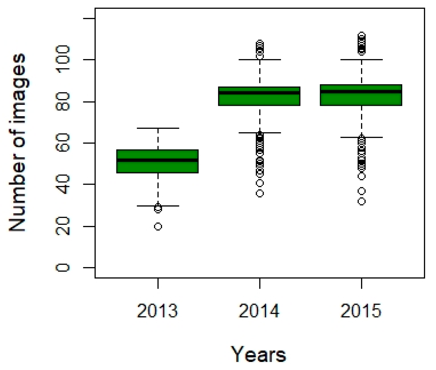
2.2.1. Landsat 8 Surface Reflectance (SR)
2.2.2. Vegetation Indices
2.3. Random Forest (RF)
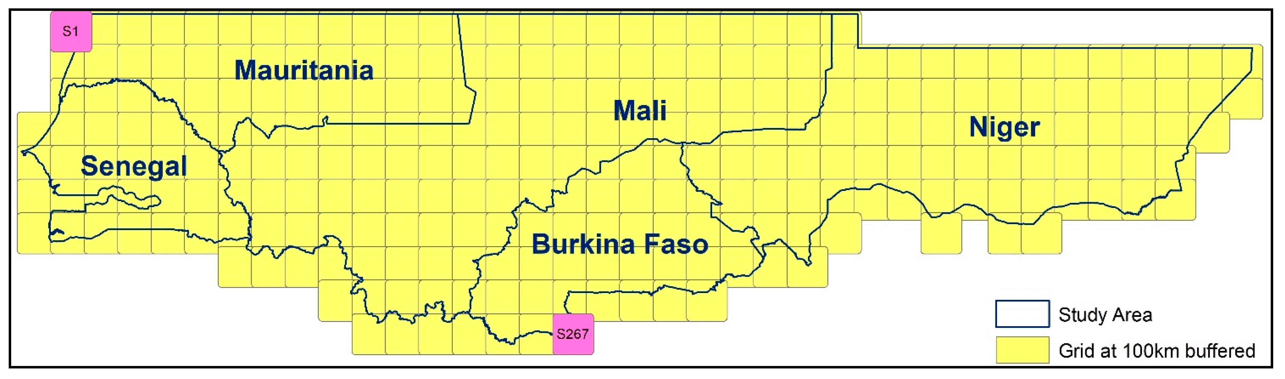
2.4. Gridding and Accuracy Metrics
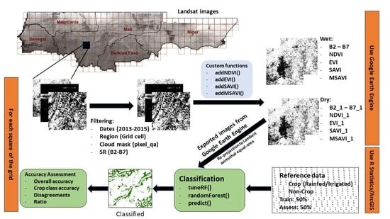
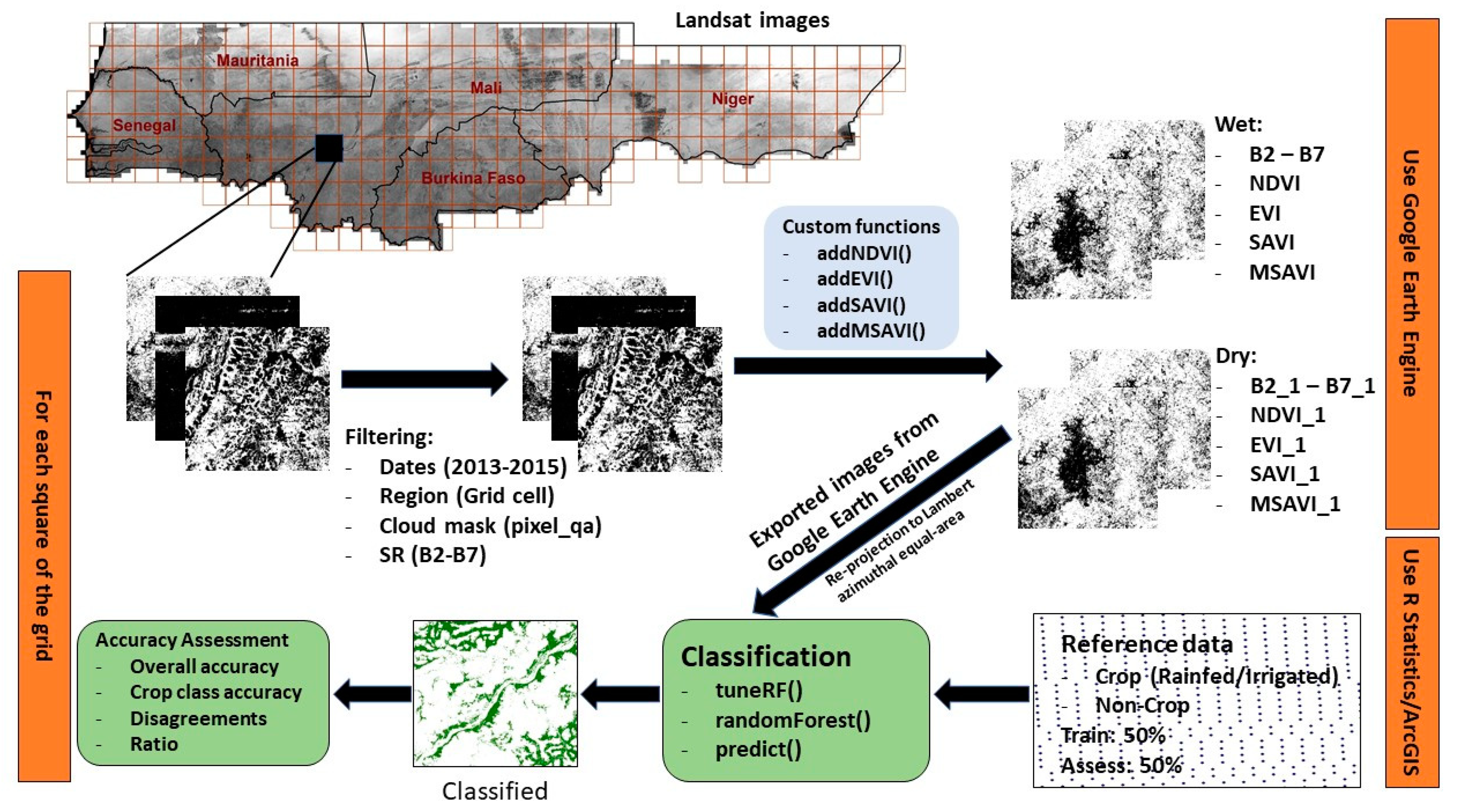
2.5. Workflow
3. Results
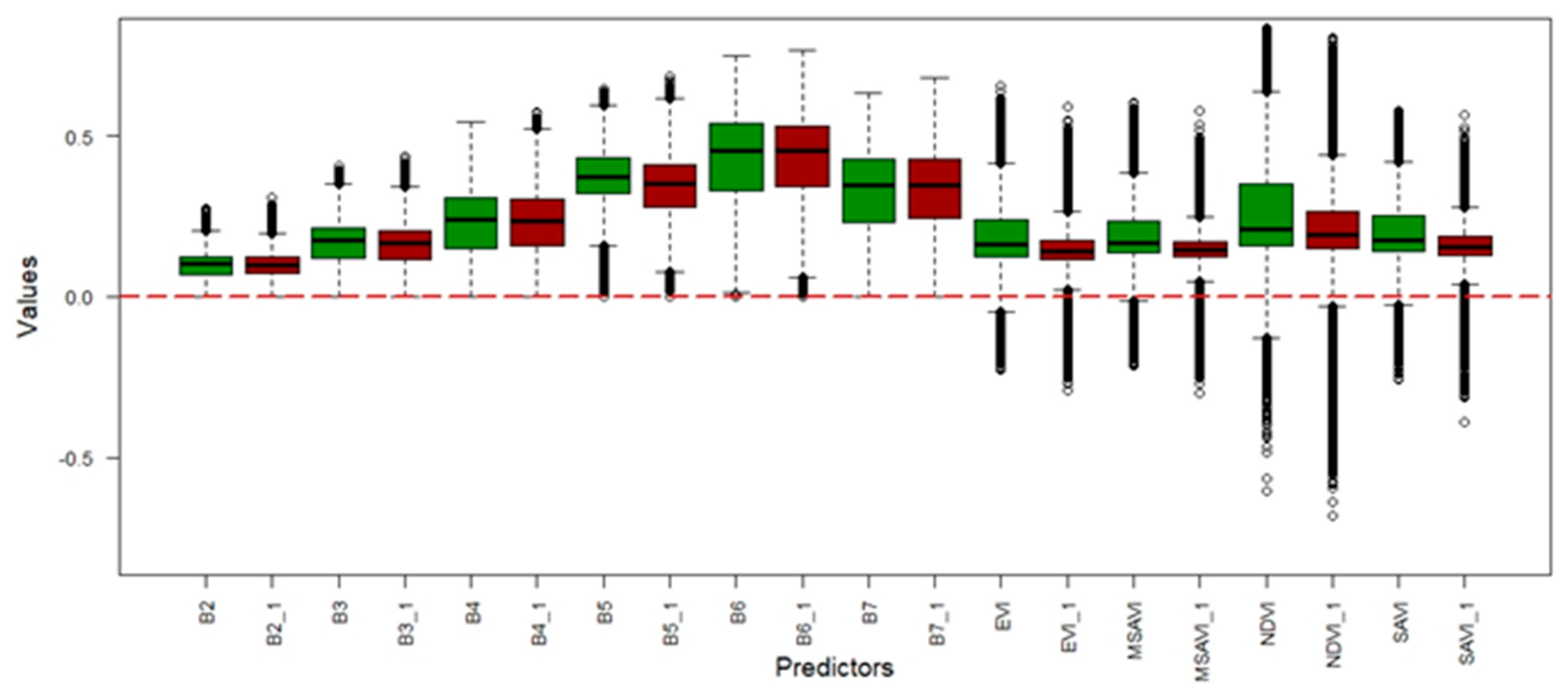
3.1. Predictors
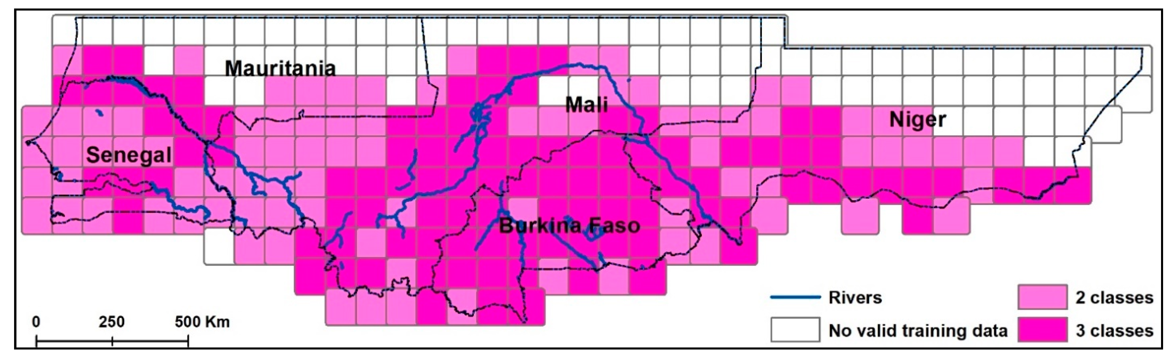
3.2. Reclassified Training Data
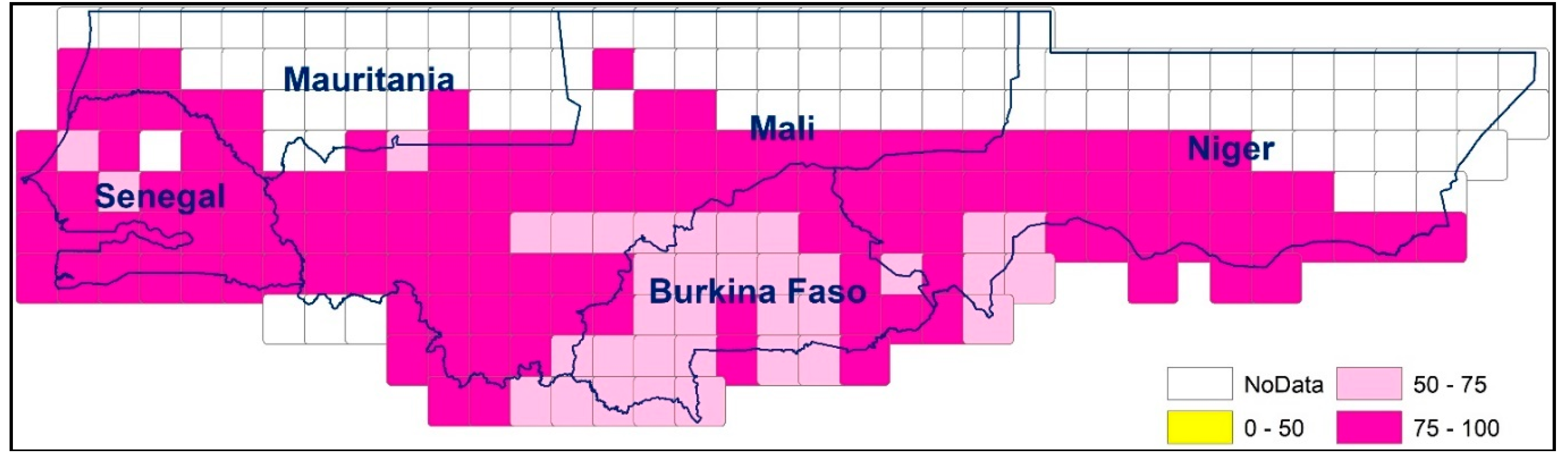
3.3. Accuracy at Grid Level
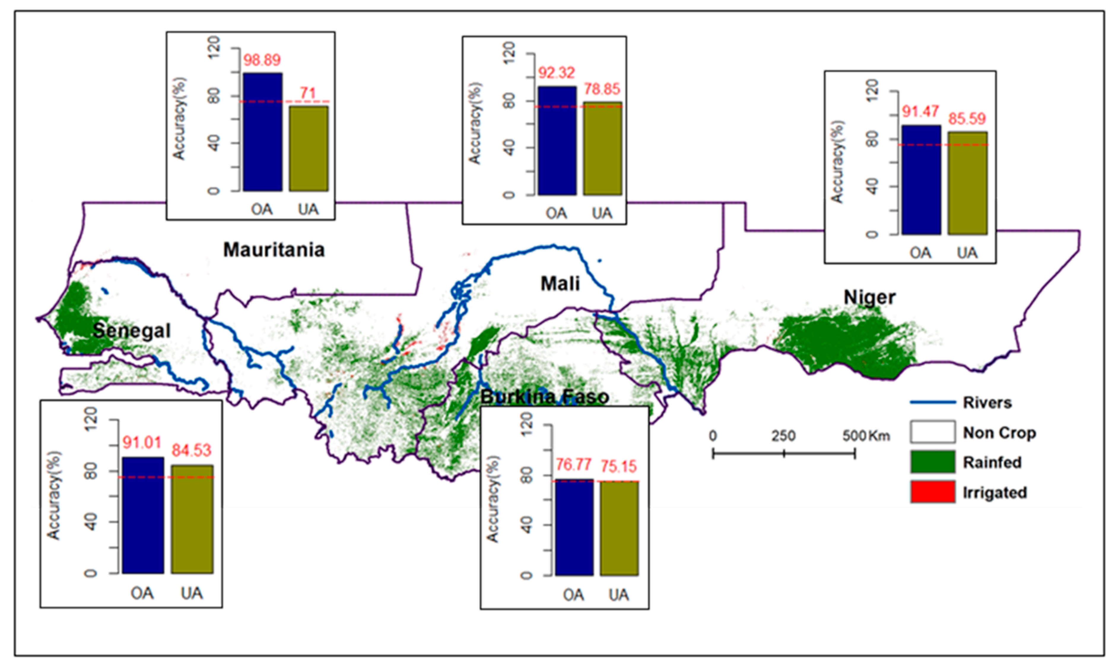
3.4. Accuracy at Country Level
4. Discussion
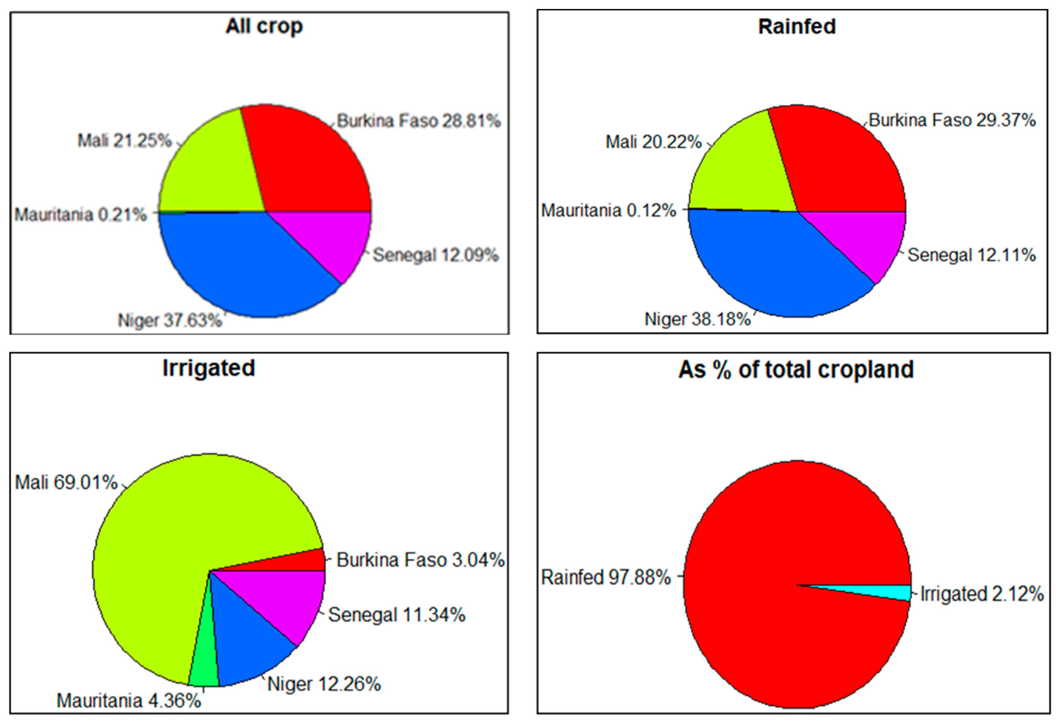
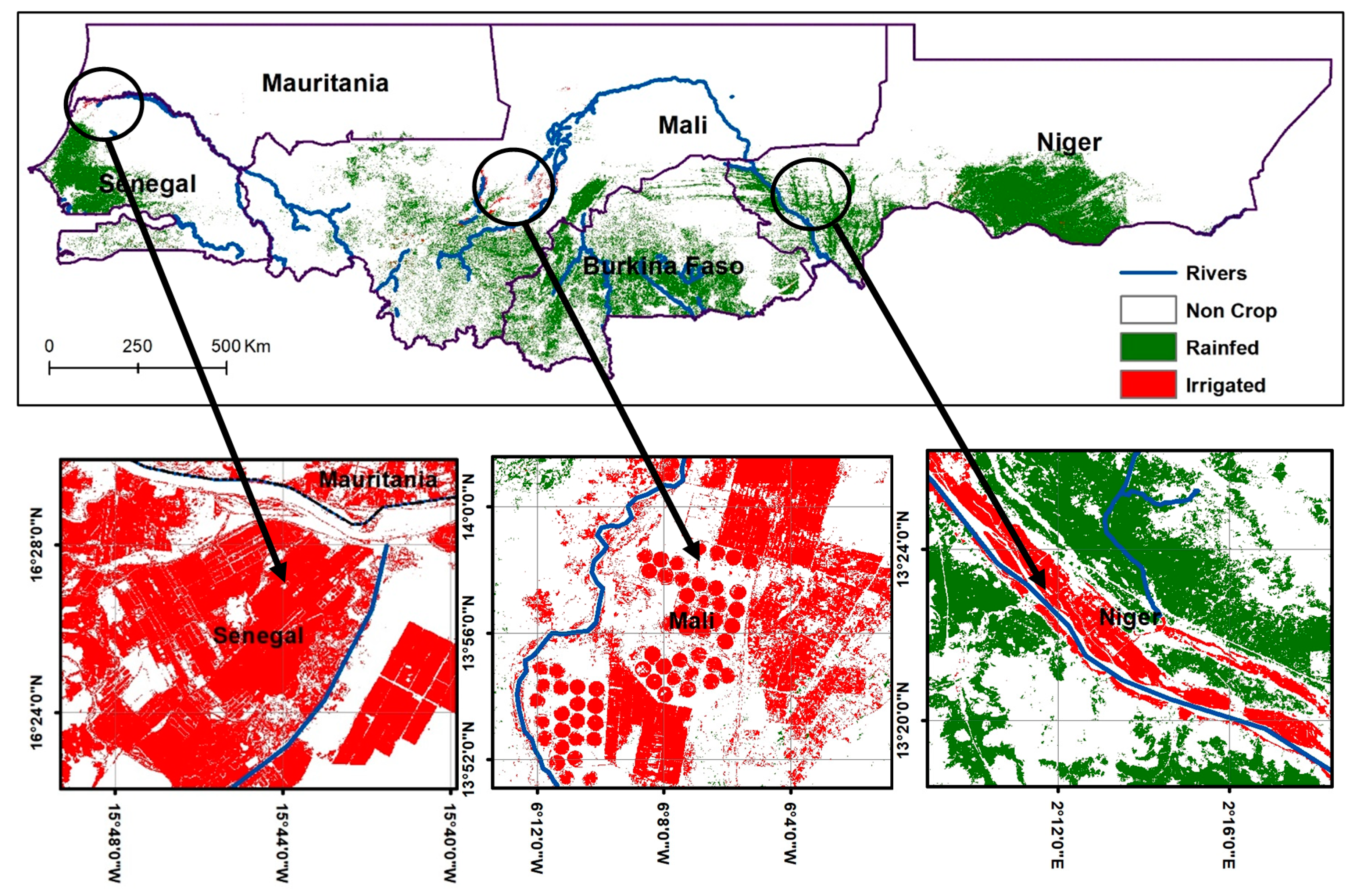
4.1. Irrigated Cropland
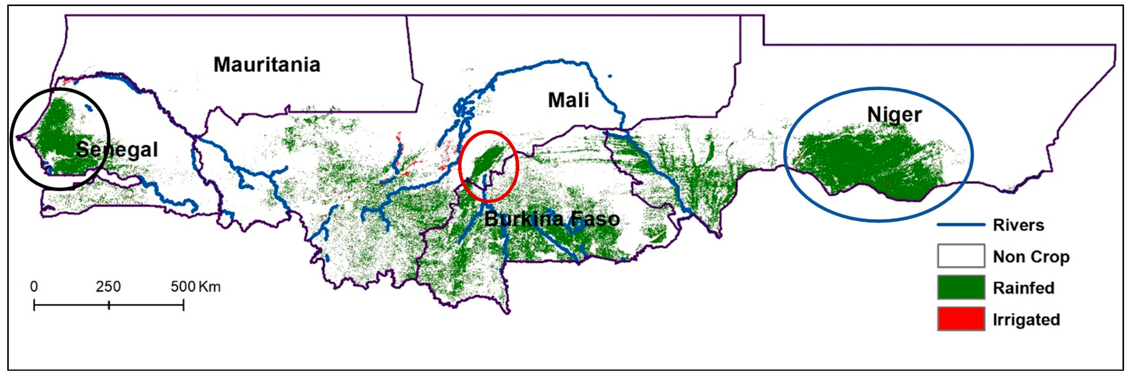
4.2. Intensive Rainfed Cropland Zones
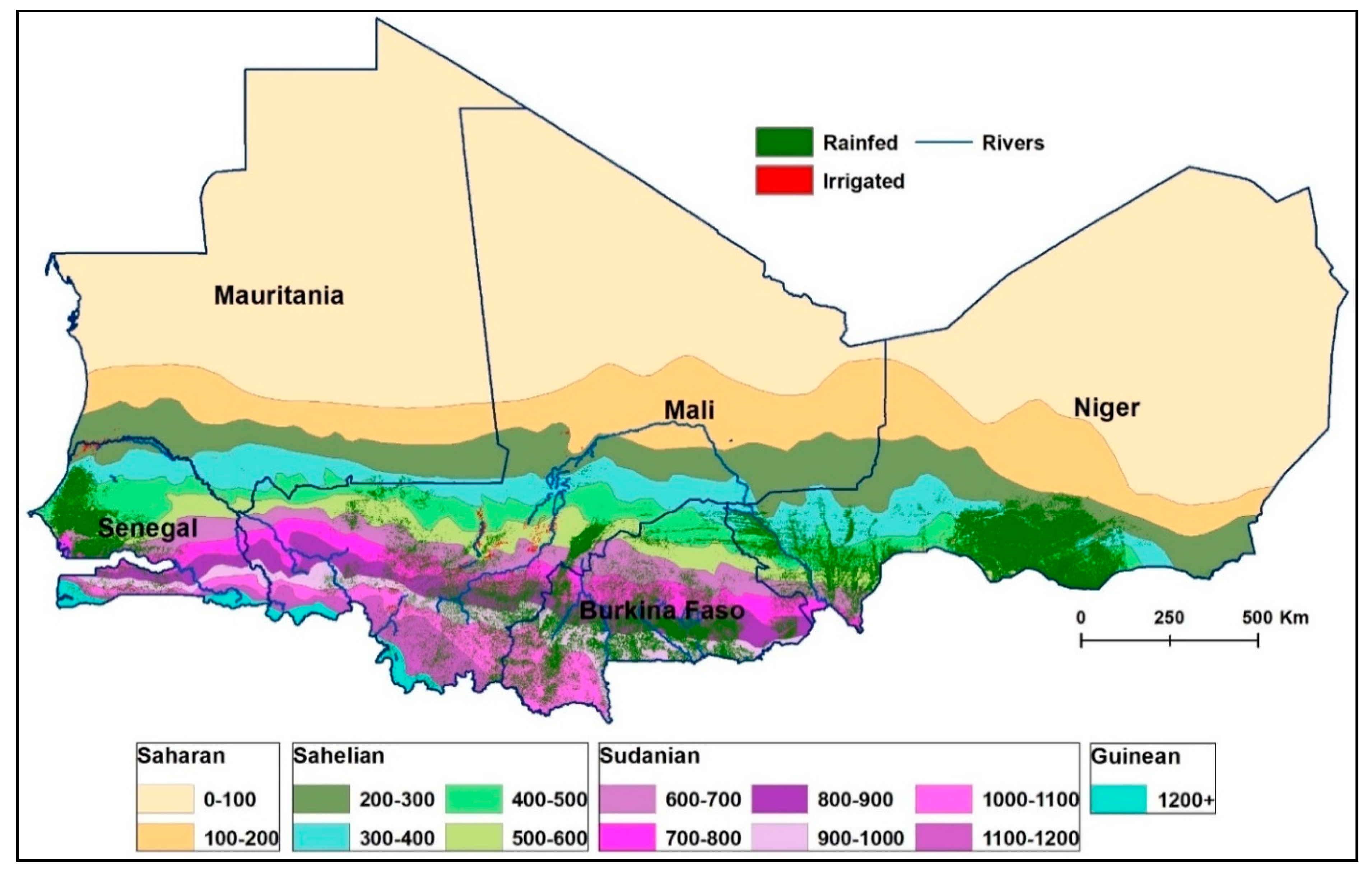
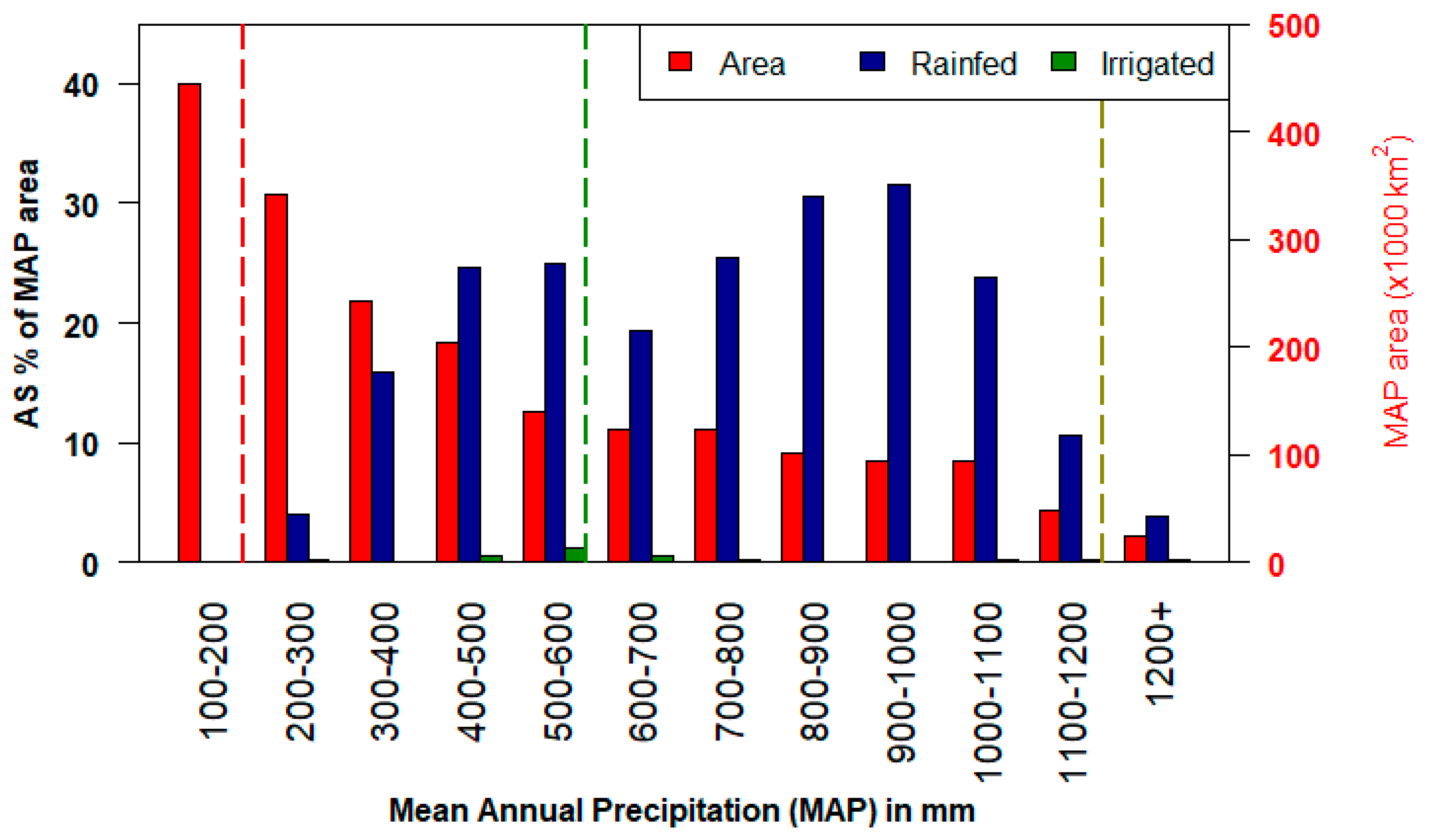
4.3. Cropland Distribution Relative to Climate and Climate Zones
4.4. Fallows in WASC30
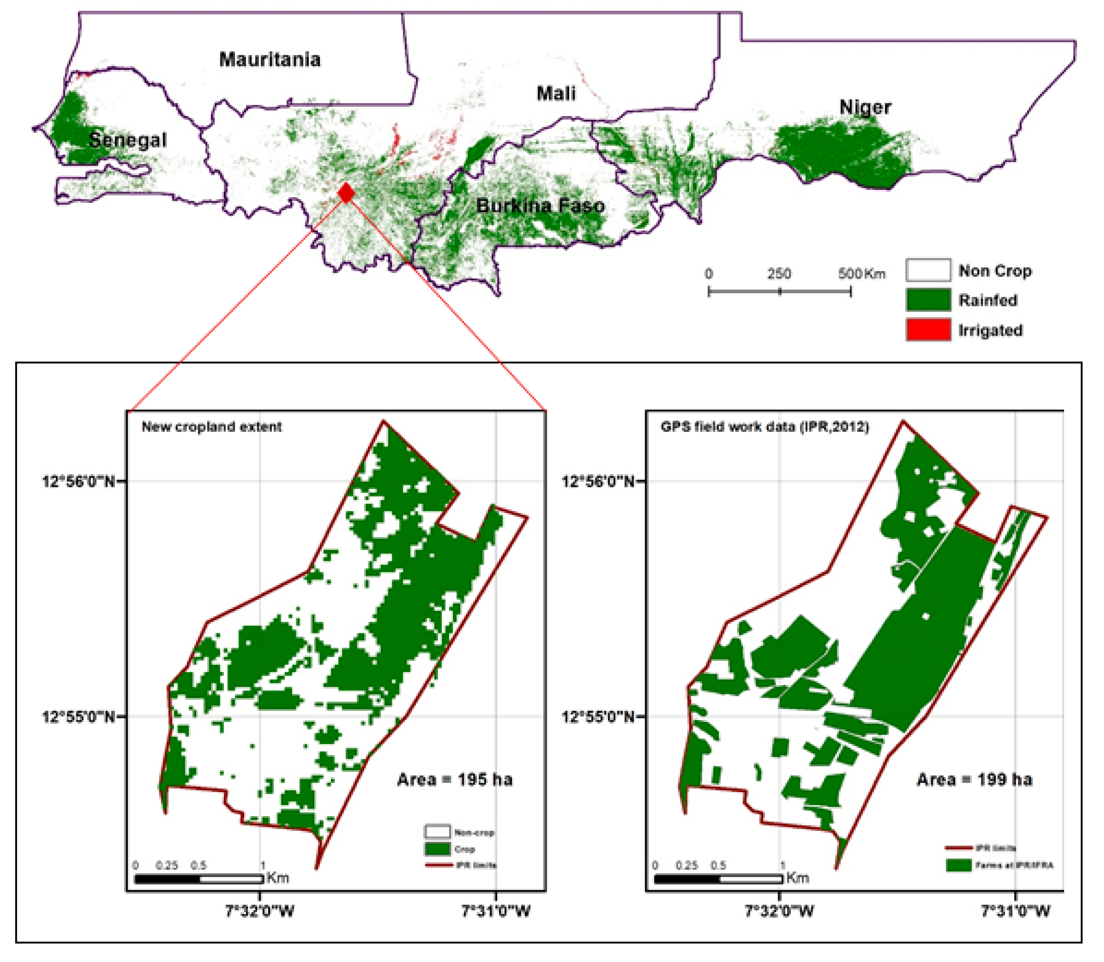
4.5. Validation Using Local Scale Data
5. Conclusions
Data Availability
Author Contributions
Funding
Acknowledgments
Conflicts of Interest
Appendix A
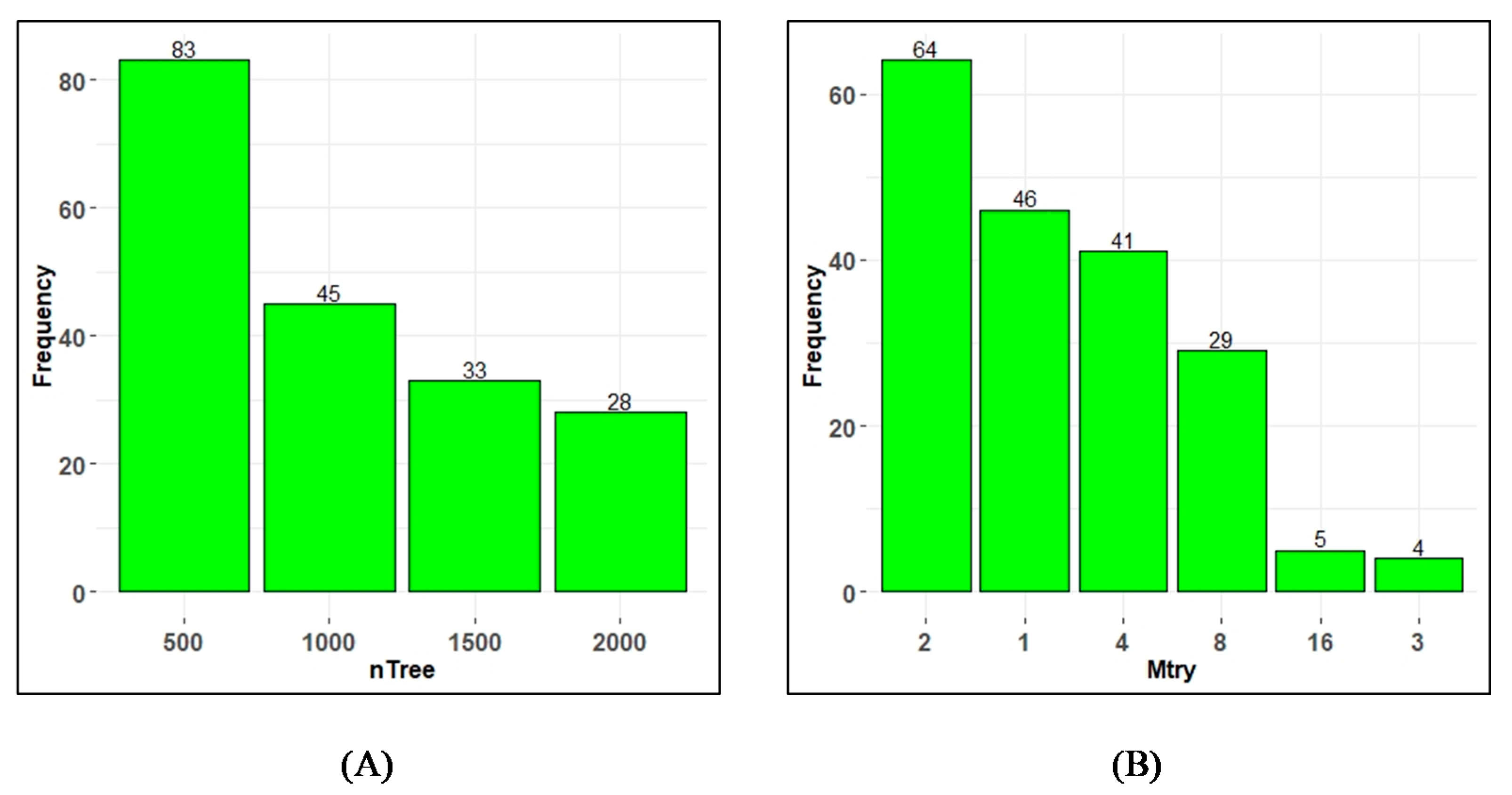
Appendix A.1. Tuning RF Major Parameters

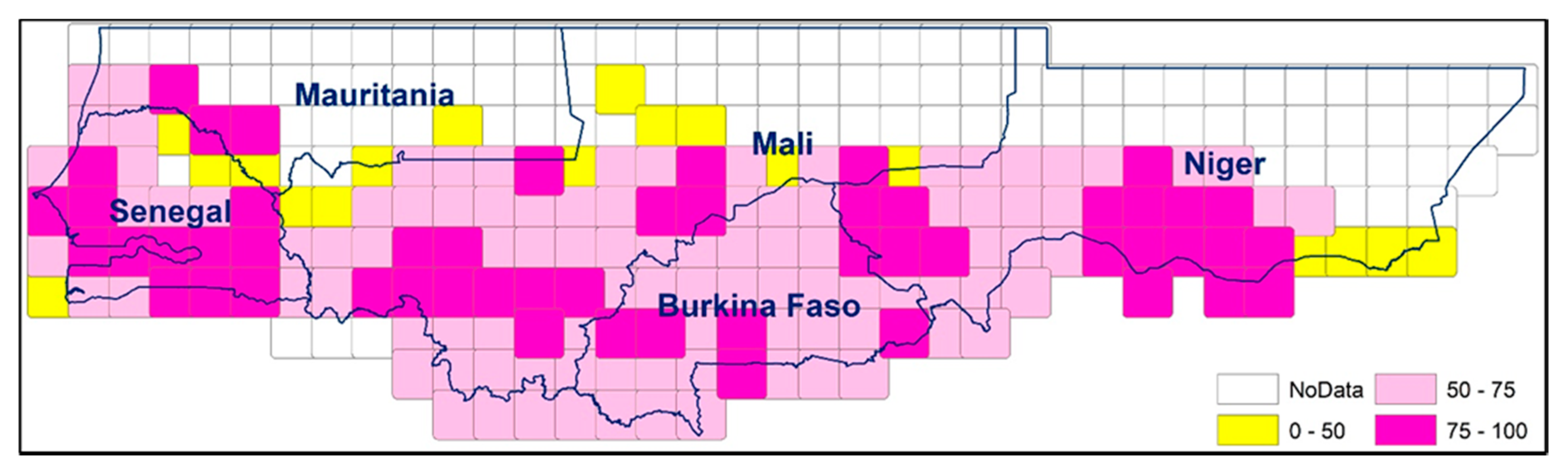
Appendix A.2. Accuracy at Grid Level


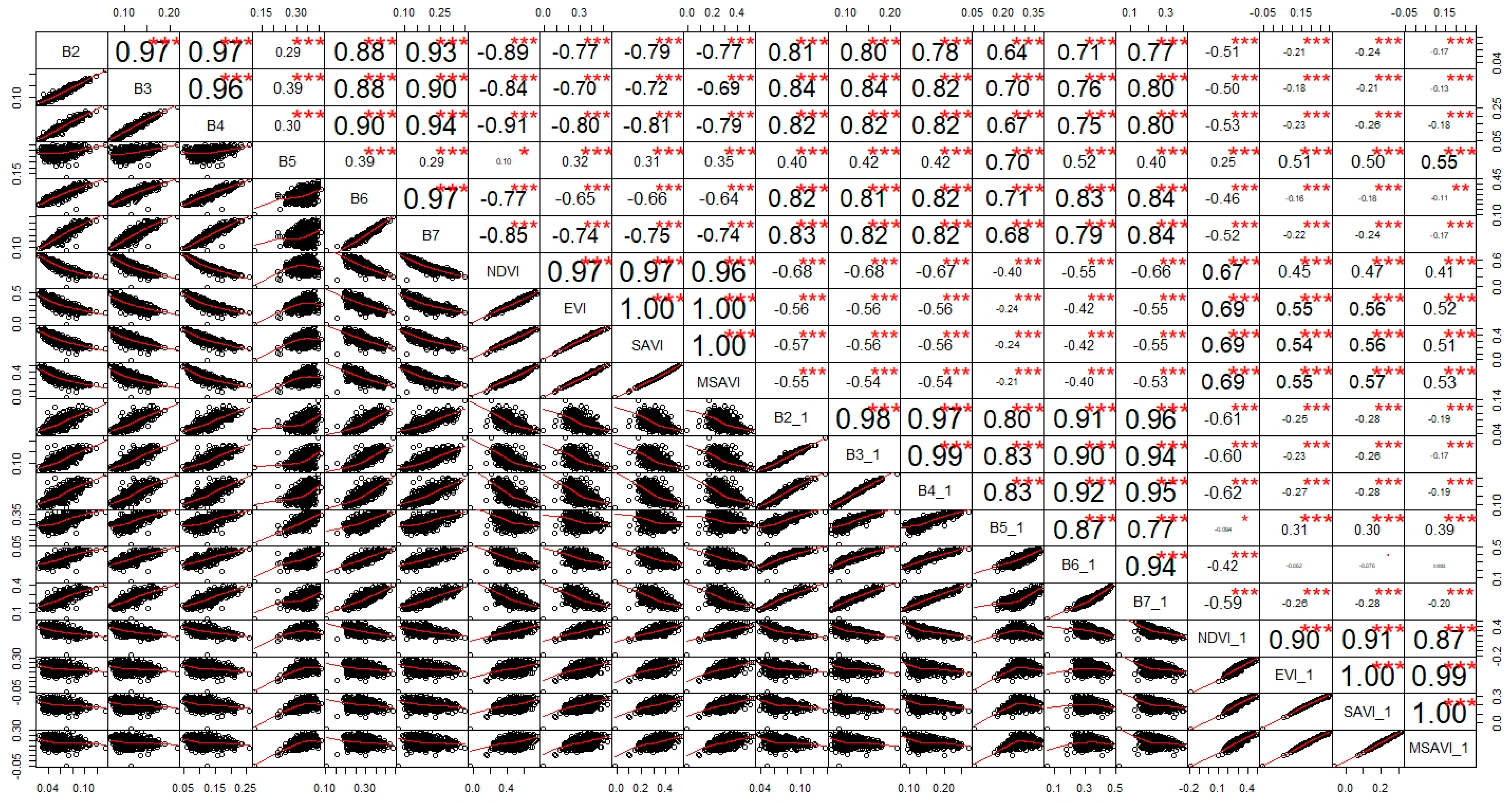
Appendix A.3. Correlated Variables/Predictors

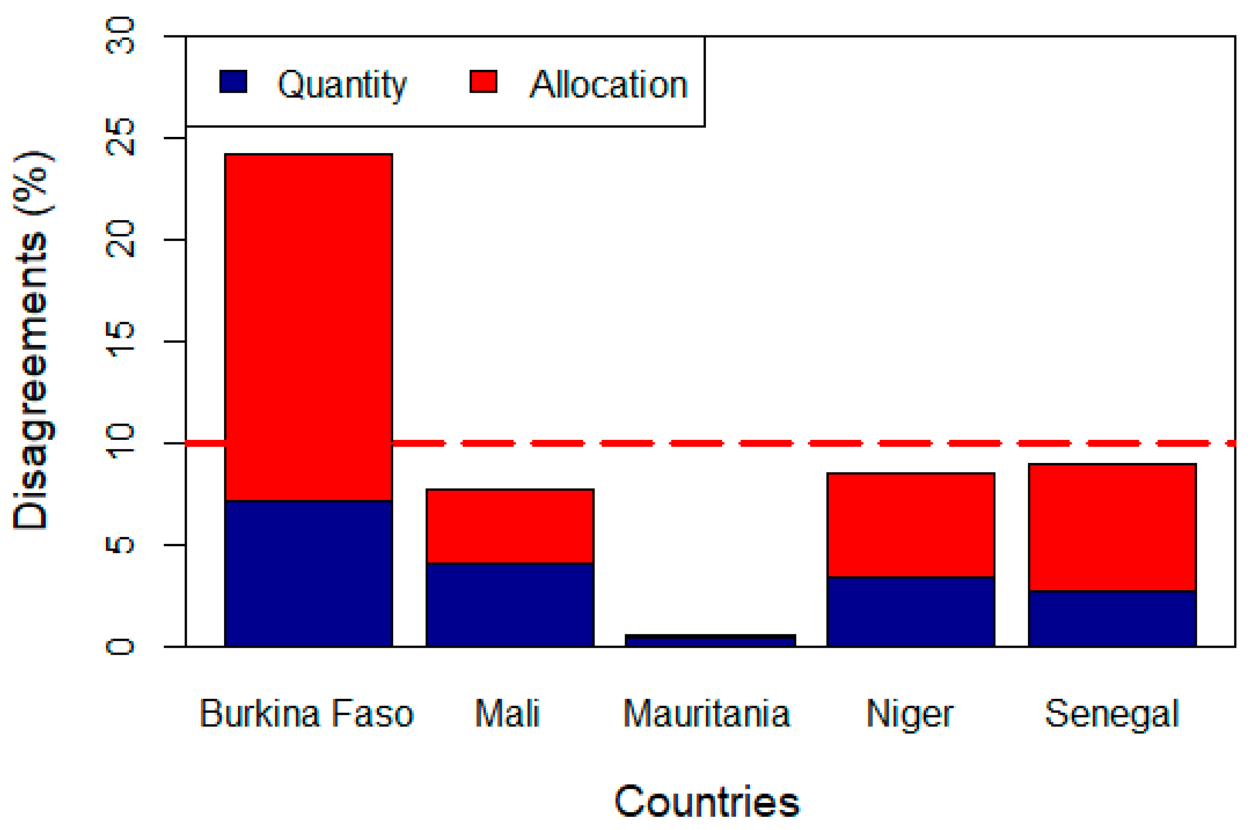
Appendix A.4. Disagreements Analysis

References
- Latham, J. FAO Land Cover Mapping Initiatives. In Proceedings of the North American Land Cover Summit, Washington, DC, USA, 20–22 September 2006; Environment and Natural Resources Service of the Food and Agriculture Organization of the United Nations (FAO): Rome, Italy, 2009; pp. 75–95. [Google Scholar]
- Thenkabail, P.; Lyon, J.G.; Turral, H.; Biradar, C. Remote Sensing of Global Croplands for Food Security; CRC Press: Boca Raton, FL, USA, 2009. [Google Scholar]
- Hollinger, F.; Staatz, J.M. Agricultural Growth in West Africa: Market and Policy Drivers; FAO: Rome, Italy; African Development Bank: Tunis, Tunisia; ECOWAS: Abuja, Nigeria, 2015. [Google Scholar]
- Atzberger, C. Advances in remote sensing of agriculture: Context description, existing operational monitoring systems and major information needs. Remote Sens. 2013, 5, 949–981. [Google Scholar] [CrossRef]
- Jones, H.G.; Vaughan, R.A. Remote Sensing of Vegetation: Principles, Techniques, and Applications; Oxford University Press: Oxford, UK, 2010. [Google Scholar]
- Lambert, M.J.; Waldner, F.; Defourny, P. Cropland mapping over Sahelian and Sudanian agrosystems: A Knowledge-based approach using PROBA-V time series at 100-m. Remote Sens. 2016, 8, 232. [Google Scholar] [CrossRef]
- Pérez-Hoyos, A.; Rembold, F.; Kerdiles, H.; Gallego, J. Comparison of global land cover datasets for cropland monitoring. Remote Sens. 2017, 9, 1118. [Google Scholar] [CrossRef]
- Xiong, J.; Thenkabail, P.S.; Tilton, J.C.; Gumma, M.K.; Teluguntla, P.; Oliphant, A.; Congalton, R.G.; Yadav, K.; Gorelick, N. Nominal 30-m cropland extent map of continental Africa by integrating pixel-based and object-based algorithms using Sentinel-2 and Landsat-8 data on google earth engine. Remote Sens. 2017, 9, 1065. [Google Scholar] [CrossRef]
- Burke, M.; Lobell, D.B. Satellite-based assessment of yield variation and its determinants in smallholder African systems. Proc. Natl. Acad. Sci. USA 2017, 114, 2189–2194. [Google Scholar] [CrossRef]
- Hong, C.; Jin, X.; Ren, J.; Gu, Z.; Zhou, Y. Satellite data indicates multidimensional variation of agricultural production in land consolidation area. Sci. Total Environ. 2019, 653, 735–747. [Google Scholar] [CrossRef]
- Löw, F.; Biradar, C.; Fliemann, E.; Lamers, J.P.A.; Conrad, C. Assessing gaps in irrigated agricultural productivity through satellite earth observations—A case study of the Fergana Valley, Central Asia. Int. J. Appl. Earth Obs. Geoinform. 2017, 59, 118–134. [Google Scholar] [CrossRef]
- Rembold, F.; Meroni, M.; Urbano, F.; Csak, G.; Kerdiles, H.; Perez-Hoyos, A.; Lemoine, G.; Leo, O.; Negre, T. ASAP: A new global early warning system to detect anomaly hot spots of agricultural production for food security analysis. Agric. Syst. 2019, 168, 247–257. [Google Scholar] [CrossRef]
- Kobayashi, N.; Tani, H.; Wang, X.; Sonobe, R. Crop classification using spectral indices derived from Sentinel-2A imagery. J. Inform. Telecommun. 2019, 1–24. [Google Scholar] [CrossRef]
- Xue, J.; Su, B. Significant remote sensing vegetation indices: A review of developments and applications. J. Sensors 2017. [Google Scholar] [CrossRef]
- Samasse, K.; Hanan, N.P.; Tappan, G.; Diallo, Y. Assessing cropland area in West Africa for agricultural yield analysis. Remote Sens. 2018, 10, 1785. [Google Scholar] [CrossRef]
- Arino, O.; Bicheron, P.; Achard, F.; Latham, J.; Witt, R.; Weber, J.L. The most detailed portrait of Earth. Eur. Space Agency 2008, 136, 25–31. [Google Scholar]
- Bartholome, E.; Belward, A.S. GLC2000: A new approach to global land cover mapping from Earth observation data. Int. J. Remote Sens. 2005, 26, 1959–1977. [Google Scholar] [CrossRef]
- Bontemps, S.; Boettcher, M.; Brockmann, C.; Kirches, G.; Lamarche, C.; Radoux, J.; Santoro, M.; Van Bogaert, E.; Wegmüller, U.; Herold, M.; et al. Multi-year global land cover mapping at 300 M and characterization for climate modelling: Achievements of the land cover component of the ESA climate change initiative. Int. Arch. Photogramm. Remote Sens. Spat. Inf. Sci. 2015, 40, 323–328. [Google Scholar] [CrossRef]
- Chen, J.; Chen, J.; Liao, A.; Cao, X.; Chen, L.; Chen, X.; He, C.; Han, G.; Peng, S.; Lu, M.; et al. Global land cover mapping at 30 m resolution: A POK-based operational approach. ISPRS J. Photogramm. Remote Sens. 2015, 103, 7–27. [Google Scholar] [CrossRef]
- Friedl, M.A.; Sulla-Menashe, D.; Tan, B.; Schneider, A.; Ramankutty, N.; Sibley, A.; Huang, X. MODIS Collection 5 global land cover: Algorithm refinements and characterization of new datasets. Remote Sens. Environ. 2010, 114, 168–182. [Google Scholar] [CrossRef]
- Fritz, S.; You, L.; Bun, A.; See, L.; McCallum, I.; Schill, C.; Perger, C.; Liu, J.; Hansen, M.; Obersteiner, M. Cropland for sub-Saharan Africa: A synergistic approach using five land cover data sets. Geophys. Res. Lett. 2011, 38. [Google Scholar] [CrossRef]
- Latham, J.; Cumani, R.; Rosati, I.; Bloise, M. Global Land Cover Share (GLC-SHARE) Database Beta-Release Version 1.0-2014; FAO: Rome, Italy, 2014. [Google Scholar]
- Tong, X.; Brandt, M.; Hiernaux, P.; Herrmann, S.; Rasmussen, L.V.; Rasmussen, K.; Tian, F.; Tagesson, T.; Zhang, W.; Fensholt, R. The forgotten land use class: Mapping of fallow fields across the Sahel using Sentinel-2. Remote Sens. Environ. 2020, 239, 111598. [Google Scholar] [CrossRef]
- Buchhorn, M.; Smets, B.; Bertels, L.; Lesiv, M.; Tsendbazar, N.E.; Herold, M.; Fritz, S. Copernicus Global Land Service: Land Cover 100 m: Epoch 2018: Africa Demo. Available online: https://zenodo.org/record/3518087#.XqgPLmgzZPY (accessed on 20 February 2020).
- Li, L.; Tsendbazar, N.; Herold, M.; Lesiv, M. Copernicus Global Land Operations “Vegetation and Energy”: Moderate Dynamic Land Cover Change Maps, Africa 2015–2018. Available online: https://land.copernicus.eu/global/sites/cgls.vito.be/files/products/CGLOPS1_PUM_LCC100m-V2.1_I3.10.pdf (accessed on 25 February 2020).
- Gorelick, N.; Hancher, M.; Dixon, M.; Ilyushchenko, S.; Thau, D.; Moore, R. Google Earth Engine: Planetary-scale geospatial analysis for everyone. Remote Sens. Environ. 2017, 202, 18–27. [Google Scholar] [CrossRef]
- Roy, D.P.; Wulder, M.A.; Loveland, T.R.; Woodcock, C.E.; Allen, R.G.; Anderson, M.C.; Helder, D.; Irons, J.R.; Johnson, D.M.; Kennedy, R.; et al. Landsat-8: Science and product vision for terrestrial global change research. Remote Sens. Environ. 2014, 145, 154–172. [Google Scholar] [CrossRef]
- Kumar, L.; Mutanga, O. Google Earth Engine applications since inception: Usage, trends, and potential. Remote Sens. 2018, 10, 1509. [Google Scholar] [CrossRef]
- Tappan, G.G.; Cushing, W.M.; Cotillon, S.E.; Mathis, M.L.; Hutchinson, J.A.; Dalsted, K. West Africa Land Use Land Cover Time Series; U.S. Geological Survey: Sioux Falls, SD, USA, 2016. [Google Scholar]
- Cotillon, S.E. West Africa Land Use and Land Cover Time Series; Fact Sheet 2017–3004; U.S. Geological Survey: Sioux Falls, SD, USA, 2017. [Google Scholar] [CrossRef]
- Cotillon, S.E.; Mathis, M.L. Mapping Land Cover Through Time with the Rapid Land Cover Mapper—Documentation and User Manual; Open File Report 2017–1012; U.S. Geological Survey: Sioux Falls, SD, USA, 2017; p. 23. [Google Scholar] [CrossRef]
- CILSS. Landscapes of West Africa—A Window on a Changing World; U.S. Geological Survey EROS: Garretson, SD, USA, 2016. [Google Scholar]
- Mardani, M.; Mardani, H.; De Simone, L.; Varas, S.; Kita, N.; Saito, T. Integration of Machine Learning and Open Access Geospatial Data for Land Cover Mapping. Remote Sens. 2019, 11, 1907. [Google Scholar] [CrossRef]
- Johnson, D.M. Using the Landsat archive to map crop cover history across the United States. Remote Sens. Environ. 2019, 232, 111286. [Google Scholar] [CrossRef]
- Azzari, G.; Lobell, D.B. Landsat-based classification in the cloud: An opportunity for a paradigm shift in land cover monitoring. Remote Sens. Environ. 2017, 202, 64–74. [Google Scholar] [CrossRef]
- Fensholt, R.; Rasmussen, K.; Nielsen, T.T.; Mbow, C. Evaluation of earth observation based long term vegetation trends—Intercomparing NDVI time series trend analysis consistency of Sahel from AVHRR GIMMS, Terra MODIS and SPOT VGT data. Remote Sens. Environ. 2009, 113, 1886–1898. [Google Scholar] [CrossRef]
- Olsson, L.; Eklundh, L.; Ardö, J. A recent greening of the Sahel—Trends, patterns and potential causes. J. Arid Environ. 2005, 63, 556–566. [Google Scholar] [CrossRef]
- Vintrou, E.; Desbrosse, A.; Bégué, A.; Traoré, S.; Baron, C.; Seen, D.L. Crop area mapping in West Africa using landscape stratification of MODIS time series and comparison with existing global land products. Int. J. Appl. Earth Obs. Geoinform. 2012, 14, 83–93. [Google Scholar] [CrossRef]
- Tucker, C.J. Red and photographic infrared linear combinations for monitoring vegetation. Remote Sens. Environ. 1979, 8, 127–150. [Google Scholar] [CrossRef]
- Huete, A.; Didan, K.; Miura, T.; Rodriguez, E.P.; Gao, X.; Ferreira, L.G. Overview of the radiometric and biophysical performance of the MODIS vegetation indices. Remote Sens. Environ. 2002, 83, 195–213. [Google Scholar] [CrossRef]
- Miura, T.; Huete, A.R.; Yoshioka, H.; Holben, B.N. An error and sensitivity analysis of atmospheric resistant vegetation indices derived from dark target-based atmospheric correction. Remote Sens. Environ. 2001, 78, 284–298. [Google Scholar] [CrossRef]
- Jiang, Z.; Huete, A.R.; Didan, K.; Miura, T. Development of a two-band enhanced vegetation index without a blue band. Remote Sens. Environ. 2008, 112, 3833–3845. [Google Scholar] [CrossRef]
- Huete, A.R. A soil-adjusted vegetation index (SAVI). Remote Sens. Environ. 1988, 25, 295–309. [Google Scholar] [CrossRef]
- Qi, J.; Chehbouni, A.; Huete, A.R.; Kerr, Y.H.; Sorooshian, S. A modified soil adjusted vegetation index. Remote Sens. Environ. 1994, 48, 119–126. [Google Scholar] [CrossRef]
- Breiman, L. Random forests. Mach. Learn. 2001, 45, 5–32. [Google Scholar] [CrossRef]
- Pontius, R.G.; Millones, M. Death to Kappa: Birth of quantity disagreement and allocation disagreement for accuracy assessment. Int. J. Remote Sens. 2011, 32, 4407–4429. [Google Scholar] [CrossRef]
- Zwart, S.J.; Leclert, L.M.C. A remote sensing-based irrigation performance assessment: A case study of the Office du Niger in Mali. Irrig. Sci. 2010, 28, 371–385. [Google Scholar] [CrossRef]
- van der Wijngaart, R.; Helming, J.; Jacobs, C.; Delvaux, P.A.G.; Hoek, S.; Gomez y Paloma, S. Irrigation and Irrigated Agriculture Potential in the Sahel: The Case of the Niger River Basin; JRC Technical Report; Publications Office of the European Union: Luxembourg, 2019. [Google Scholar]
- Woodhouse, P.; Ganho, A.S. Is Water the Hidden Agenda of Agricultural Land Acquisition in Sub-Saharan Africa. In Proceedings of the International Conference on Global Land Grabbing, Sussex, UK, 6–8 April 2018; Land Deals Politics Initiative: The Hague, The Netherlands, 2011; pp. 1–19. [Google Scholar]
- Thibaud, B. Le pays dogon au Mali: De l’enclavement à l’ouverture ? Espac. Popul. Soc. 2005, 1, 45–56. [Google Scholar] [CrossRef]
- Issoufou, W.S.; Mahamane, A.; Ousseini, I. La Surveillance Ecologique et Environnementale au Niger: Un instrument d’aide à la décision. Options Méditerr. Sér. B. Etudes Rech. 2012, 68, 219–230. [Google Scholar]
- RNCA-NIGER. Le Zonage Agro-Ecologique du NIGER. 2019. Available online: https://reca-niger.org/IMG/pdf/Le_zonage_agroecologique_du_Niger_Extraits.pdf (accessed on 15 January 2020).
- FALL, C.A. État des Ressources Phytogénétiques pour l’Alimentation et l’Agriculture dans le Monde: Contribution du Sénégal au Second Rapport. 2009. Available online: http://www.fao.org/pgrfa-gpa-archive/sen/docs/senegal2.pdf (accessed on 15 January 2020).
- Bouzidi, B. Viability of solar or wind for water pumping systems in the Algerian Sahara regions—Case study Adrar. Renew. Sustain. Energy Rev. 2011, 15, 4436–4442. [Google Scholar] [CrossRef]
- Hamidat, A.; Benyoucef, B.; Hartani, T. Small-scale irrigation with photovoltaic water pumping system in Sahara regions. Renew. Energy 2003, 28, 1081–1096. [Google Scholar] [CrossRef]
- Sidibe, A. L’Etat des Ressources Phytogénétiques pour l’Alimentation et l’Agriculture au Mali—2007; Deuxième Rapport National; FAO: Rome, Italy, 2007. [Google Scholar]
- Pal, M. Random forest classifier for remote sensing classification. Int. J. Remote Sens. 2005, 26, 217–222. [Google Scholar] [CrossRef]
- Richards, J.A.; Jia, X. Remote Sensing Digital Image Analysis; Springer Nature Switzerland AG: Basel, Switzerland, 1999; Volume 3. [Google Scholar]


| Name | Band description | Wavelength (μm) |
|---|---|---|
| B2 | Band 2 (blue) surface reflectance | 0.452–0.512 |
| B3 | Band 3 (green) surface reflectance | 0.533–0.590 |
| B4 | Band 4 (red) surface reflectance | 0.636–0.673 |
| B5 | Band 5 (near infrared) surface reflectance | 0.851–0.879 |
| B6 | Band 6 (shortwave infrared 1) surface reflectance | 1.566–1.651 |
| B7 | Band 7 (shortwave infrared 2) surface reflectance | 2.107–2.294 |
| pixel_qa | Pixel quality attributes generated from the CFMASK algorithm. | --- |
| Wet Period (Growing Period) | Dry period | |
|---|---|---|
| Surface Reflectance | B2, B3, B4, B5, B6, B7 | B2_1, B3_1, B4_1, B5_1, B6_1, B7_1, |
| Vegetation Indices | NDVI, EVI, SAVI, MSAVI | NDVI_1, EVI_1, SAVI_1, MSAVI_1 |
| Overall accuracy | ||||
|---|---|---|---|---|
| No data | 0–50 | 50–75 | 75–100 | |
| Number of cells | 99 | 0 | 36 | 132 |
| Average OA | - | - | 70.59 | 87.07 |
| User’s accuracy | ||||
| Number of cells | 99 | 18 | 98 | 52 |
| Average UA | - | 22.73 | 64.10 | 82.95 |
| Burkina Faso | Mali | Mauritania | Niger | Senegal | Total | |
|---|---|---|---|---|---|---|
| Rainfed crop (km2) | 90,799 | 62,513 | 372 | 118,022 | 37,434 | 309,139 |
| Irrigated crop (km2) | 203 | 4615 | 291 | 820 | 758 | 6688 |
| Total | 91,002 | 67,128 | 664 | 118,841 | 38,192 | 315,827 |
| Saharan | Sahelian | Sudanian | Guinean | |
|---|---|---|---|---|
| % Area | 61.02 | 23.50 | 14.85 | 0.63 |
| % Rainfed | 0.00 | 14.79 | 24.54 | 3.78 |
| % Irrigated | 0.01 | 0.48 | 0.26 | 0.17 |
| % All Cropland | 0.01 | 15.27 | 24.80 | 3.95 |
© 2020 by the authors. Licensee MDPI, Basel, Switzerland. This article is an open access article distributed under the terms and conditions of the Creative Commons Attribution (CC BY) license (http://creativecommons.org/licenses/by/4.0/).
Share and Cite
Samasse, K.; Hanan, N.P.; Anchang, J.Y.; Diallo, Y. A High-Resolution Cropland Map for the West African Sahel Based on High-Density Training Data, Google Earth Engine, and Locally Optimized Machine Learning. Remote Sens. 2020, 12, 1436. https://doi.org/10.3390/rs12091436
Samasse K, Hanan NP, Anchang JY, Diallo Y. A High-Resolution Cropland Map for the West African Sahel Based on High-Density Training Data, Google Earth Engine, and Locally Optimized Machine Learning. Remote Sensing. 2020; 12(9):1436. https://doi.org/10.3390/rs12091436
Chicago/Turabian StyleSamasse, Kaboro, Niall P. Hanan, Julius Y. Anchang, and Yacouba Diallo. 2020. "A High-Resolution Cropland Map for the West African Sahel Based on High-Density Training Data, Google Earth Engine, and Locally Optimized Machine Learning" Remote Sensing 12, no. 9: 1436. https://doi.org/10.3390/rs12091436
APA StyleSamasse, K., Hanan, N. P., Anchang, J. Y., & Diallo, Y. (2020). A High-Resolution Cropland Map for the West African Sahel Based on High-Density Training Data, Google Earth Engine, and Locally Optimized Machine Learning. Remote Sensing, 12(9), 1436. https://doi.org/10.3390/rs12091436