Article

Mapping Natural Forest Remnants with Multi-Source and Multi-Temporal Remote Sensing Data for More Informed Management of Global Biodiversity Hotspots

1
Department of Geography and Geology, University of Turku, FI-20014 Turku, Finland
2
Department of Geosciences and Geography, University of Helsinki, FI-00014 Helsinki, Finland
*
Author to whom correspondence should be addressed.
Remote Sens. 2020, 12(9), 1429; https://doi.org/10.3390/rs12091429
Submission received: 8 March 2020 / Revised: 25 April 2020 / Accepted: 29 April 2020 / Published: 1 May 2020
(This article belongs to the Section Remote Sensing Image Processing)

Abstract

:
Global terrestrial biodiversity hotspots (GBH) represent areas featuring exceptional concentrations of endemism and habitat loss in the world. Unfortunately, geospatial data of natural habitats of the GBHs are often outdated, imprecise, and coarse, and need updating for improved management and protection actions. Recent developments in satellite image availability, combined with enhanced machine learning algorithms and computing capacity, enable cost-efficient updating of geospatial information of these already severely fragmented habitats. This study aimed to develop a more accurate method for mapping closed canopy evergreen natural forest (CCEF) of the Eastern Arc Mountains (EAM) ecoregion in Tanzania and Kenya, and to update the knowledge on its spatial extent, level of fragmentation, and conservation status. We tested 1023 model possibilities stemming from a combination of Sentinel-1 (S1) and Sentinel-2 (S2) satellite imagery, spatial texture of S1 and S2, seasonality derived from Landsat-8 time series, and topographic information, using random forest modelling approach. We compared the best CCEF model with existing spatial forest products from the EAM through independent accuracy assessment. Finally, the CCEF model was used to estimate the fragmentation and conservation coverage of the EAM. The CCEF model has moderate accuracy measured in True Skill Statistic (0.57), and it clearly outperforms other similar products from the region. Based on this model, there are about 296,000 ha of Eastern Arc Forests (EAF) left. Furthermore, acknowledging small forest fragments (1–10 ha) implies that the EAFs are more fragmented than previously considered. Currently, the official protection of EAFs is disproportionally targeting well-studied mountain blocks, while less known areas and small fragments are underrepresented in the protected area network. Thus, the generated CCEF model should be used to design updates and more informed and detailed conservation allocation plans to balance this situation. The results highlight that spatial texture of S2, seasonality, and topography are the most important variables describing the EAFs, while spatial texture of S1 increases the model performance slightly. All in all, our work demonstrates that recent developments in Earth observation allows significant enhancements in mapping, which should be utilized in areas with outstanding biodiversity values for better forest and conservation planning.

Graphical Abstract

1. Introduction

Global terrestrial biodiversity hotspots (GBH) represent areas featuring exceptional concentrations of endemism and habitat loss in the world [1]. The 36 GBHs recognized today harbor 50% of vascular plants and 42% of terrestrial vertebrates in only 2.3% of the world’s land area. The majority of GBHs are tropical forest ecosystems that are not only valuable for their biodiversity but also for their role in hydrological and carbon cycles, moderating environmental extremes, and provision of other ecosystem services for hundreds of millions of people [1,2,3]. Habitat loss and fragmentation due to the expansion of anthropogenic land use is considered as the greatest contemporary threat to these forested GBHs [4,5,6,7]. Recent studies predict that fragmentation, i.e., the division of habitat into smaller and more isolated patches may become the future norm for tropical forest ecosystems [8,9,10]. It is widely accepted that limited conservation resources should be focused on these areas to prevent global environmental degradation and loss of biodiversity [1,11,12].
Forest fragmentation causes multiple impacts for ecological resilience of tropical forests through direct habitat loss, reduction of fragment size, increase in edge effects, and spatial isolation, while fragmented forests are also prone to further deforestation [8,9,13,14]. From a conservation perspective, small natural forest fragments are considered less important compared to large and intact natural forest patches [15,16,17]. However, small fragments are likely to harbor more irreplaceable unique or rare biodiversity values compared to an area of the same size in intact landscape [18,19]. Furthermore, they maintain the previous geographical extent of the habitat and act as stepping stones for wildlife contributing to short- and long-term species persistence [18,19]. In this context, the forest conservation and management plans should recognize the contribution of both small and large forest patches into the overall ecosystem persistence, especially in the areas of outstanding biodiversity values such as the GBHs [11,12].
Unfortunately, geospatial data on natural vegetation of GBHs are generally outdated, imprecise, and coarse [20]. While recent Landsat-based assessments have provided relatively fine-scale measures of global forest coverage and dynamics [21], global intact forest landscapes [22], and global hinterland forests [23], they represent weakly the forest habitats, in particular GBH due to, e.g., generalized semantics of forests or large minimum mappable unit. Especially in fragmented GBHs, small, linear, and isolated forest fragments are often underrepresented in such data sets [8,22,23,24]. To make well-informed decisions on management and conservation, geospatial data must be able to discriminate natural undisturbed forests from other forest types (e.g., plantations or degraded forests) and produce reliable estimations on forest coverage and fragmentation, which is not possible through some global data sets [20,21]. Thus, updated forest mapping methods increasing the spatial accuracy of the extent and boundaries of natural forest remnants are needed at contextually relevant scale. This is vital for the establishment of cost-efficient and accurate monitoring methods of forest changes such as detection of canopy disturbances [25,26].
Recent advances in satellite data availability and temporal, radiometric, and spatial resolution provided by the Sentinels, has made it possible to significantly improve the identification of small fragments in tropical forests [26,27]. Furthermore, methodological advances, such as time series analysis of optical satellite imagery or synergistic approaches that combine the advantages of optical and synthetic aperture radar (SAR) imagery, have shown to improve vegetation classification in tropical areas when detecting detailed vegetation characteristics [28,29,30,31,32]. Moreover, advances in machine learning algorithms, such as random forests, have improved models regarding forest distribution, types, and attributes [33,34]. The emergence of cloud computing platforms, such as Google Earth Engine (GEE), have made processing of enormous data volumes with complex algorithms technically possible [35]. The development of applications such as Google Earth and Bing maps allows access to global coverage of very high-resolution (VHR) satellite imagery, facilitating rigorous reference and validation sample collection over large areas [36]. Altogether, these developments have diversified the opportunities for repeatable high-resolution forest mapping and monitoring approaches [21,25]. Such approaches are vital, especially in the countries representing Global South where access to data and computing power is restricted.
The Eastern Arc Mountain (EAM) forests of Tanzania and Kenya are a major component of the East Afromontane biodiversity hotspot, one of the most fragmented GBHs in the world [37,38,39]. Previous studies have estimated that almost 80% of the EAM forests have been cleared [40,41,42,43]. Several studies have evaluated the historical and present forest coverage of Eastern Arc Forests (EAFs) [37,43,44,45]. More recently, Newmark and McNeally [39] evaluated the amount and distribution of natural forest fragments, reporting a higher number of smaller fragments across the EAM. However, the spatial distribution of small remnants, as well as open gaps within large intact forest patches, remains unknown in the EAM and their role in promoting connectivity and significance as nodal points for habitat regeneration and rehabilitation has been unaccounted [19,39,46].
In this study, we developed a high-resolution (10 m) closed canopy evergreen natural forest (CCEF) model (generated from 10–30 m data) across the EAM through testing optimal combinations of multi-temporal and multi-sensor satellite imagery and ancillary geospatial data. The CCEF model was then compared to previous spatial estimates of the EAF and used to evaluate the conservation status of the natural forests in the EAM. Results were discussed in the light of conservation and management actions. Furthermore, we discussed the need and potential of similar mapping approaches in updating the spatial information of other invaluable tropical forest ecosystems located in generally data-scarce Global South.

2. Methods and Study Area
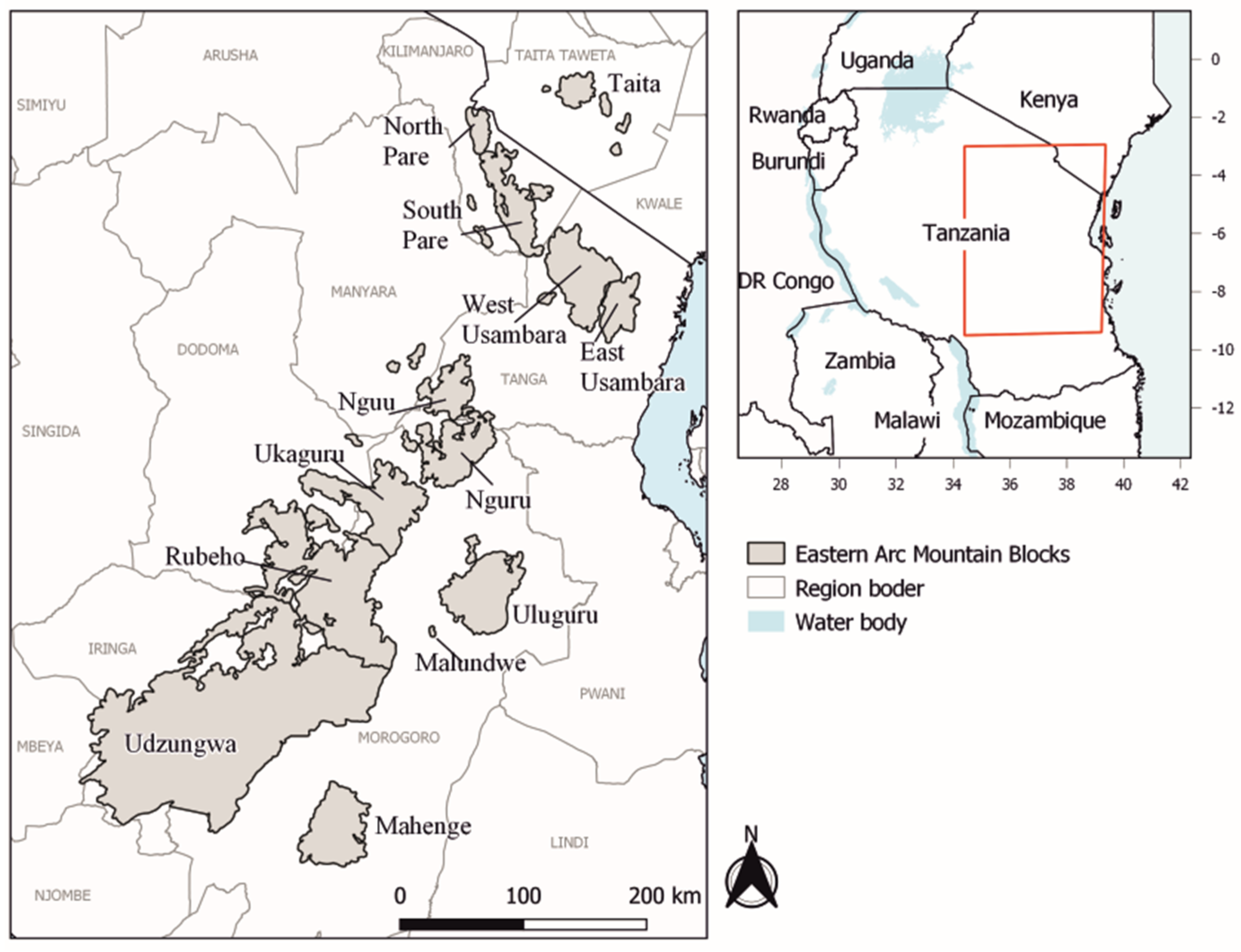
2.1. Study Area

The Eastern Arc Mountains consist of 13 separate mountain blocks that stretch geographically from southwest Tanzania to south Kenya (Figure 1). The mountains share similar geology and rainfall patterns, governed by the Indian Ocean climatic regime, supporting humid montane forest habitats [38,47]. The EAM area holds outstanding biodiversity value, globally ranked among the most important areas for the conservation of endemic birds and plants [11,42,48], and hosting at least 96 endemic vertebrate species [38] and four endemic or near-endemic primate species [49,50]. At the same time, millions of people depend for their livelihood on these tropical mountain forest ecosystems that provide a source of water, wood for fuel and construction, charcoal, handicrafts, and medicines [51,52]. Deforestation and forest degradation are the biggest threats to EAFs. Fortunately, a majority of the remaining EAFs are protected via government and private protection areas, and recently many of the nature and forest reserves have been coded into the International Union for Conservation of Nature (IUCN) system [53]. Nevertheless, approximately 25% of the EAFs are located outside of the protected areas [43,47,52].

2.2. Methods

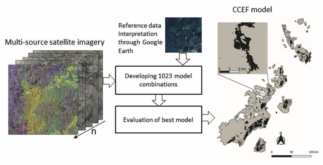
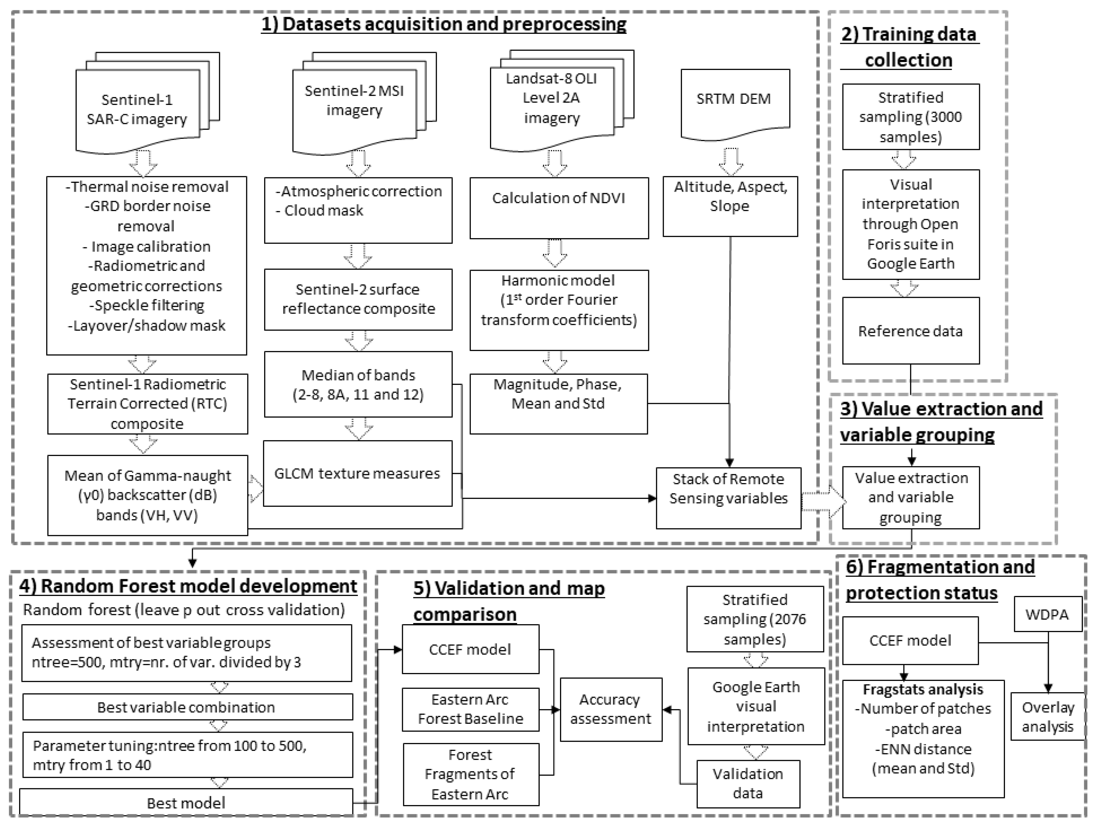
2.2.1. Methodological Design

The CCEF model was based on freely available satellite images and geospatial data sets. An overview of the methodological design is illustrated in Figure 2. The approach was divided into six phases: (1) Data sets’ acquisition and preprocessing, (2) training data collection, (3) value extraction and variable grouping, (4) random forest model development, (5) validation and map comparison, and (6) fragmentation and protection status. The sections below describe the phases in more detail.

2.2.2. Data Sets and Preprocessing

As optical Earth observation data, we used Sentinel-2 Multi-Spectral Instrument (MSI) imagery with spatial resolution of 10–20 m [54]. We screened visually the entire catalogue of Sentinel-2 imagery available for the study area to extract only images with low cloud coverage on the EAFs, as image pre-selection has shown to improve the quality of pixel-based composites [55]. Due to frequent cloud cover in the study area, we had to expand our image acquisition for multiple years (2016–2018). Altogether, 45 Sentinel-2 top-of-atmosphere (TOA) Level-1C images (Supplementary Materials, Table S1) were downloaded from the Copernicus Open Access Hub of European Space Agency (ESA) and atmospherically corrected with Sen2Cor processor. Sen2Cor algorithm associates image-derived atmospheric properties with the precomputed look-up tables [56]. Default settings of Sen2Cor were used. The corrected images were imported to GEE and masked for clouds and shadows using the available quality band of Sentinel-2 and blue band thresholding. To avoid remaining cloud and shadow effects, a median pixel composite was calculated from the images and all the visible (B2–B4), near-infrared (NIR), red edge (B8, B8a, B5–B7), and shortwave infrared (SWIR) bands (B11 and B12) were extracted for further analysis as these bands have shown to distinguish effectively spectral variance in forest canopies [57,58].
As radar data, we used the available Sentinel-1 SAR-C Level-1 Interferometric Wide (IW) ground range detected (GRD) dual-polarized VV (vertical transmit-vertical receive), VH (vertical transmit-horizontal receive) imagery with spatial resolution of 10 m, which were acquired from the Copernicus Open Access Hub [59]. Sentinel-1 bands are sensitive to surface structure and moisture content and have shown useful in forest coverage and structure mapping [60]. Altogether, 33 images were retrieved from 28 September 2008–30 September 2017 (Supplementary Materials, Table S1) since September represents the dry period throughout the study area with similar conditions considering vegetation phenology and land use practices. The number of images covering each block varied from three to five depending on the availability of images. The preprocessing of the SAR images was conducted in Sentinel Application Platform (SNAP) [61] and included thermal noise removal, image border noise removal, image calibration, radiometric and geometric corrections, and speckle filtering in order to derive gamma-naught backscatter values (dB) [62]. We used the default settings in each processing step. The images were imported to GEE and masked for layover and shadow. A mean pixel mosaic was calculated for the whole study area and VV and VH bands were extracted for further analysis.
Time series of Earth observation products have shown to capture seasonal trends of land cover features and improve land cover classifications [63]. Our aim was to derive annual phenological response of vegetation to discriminate between the closed canopy evergreen forest and other type of vegetation. We used Landsat-8 Operational Land Imager (OLI) Level 1A surface reflectance products to calculate Normalized Difference Vegetation Index (NDVI) for the entire Landsat-8 epoch in GEE. The NDVI time series was then fitted with a harmonic model using Fourier transform coefficients of first order constituting in simple phenological cycles [64]. Four seasonal variables (magnitude, phase, mean, and standard deviation) were derived from the fitted NDVI model.
Texture measures of satellite images are sensitive to forest structure (variation in crown size, crown shadow, spacing, and cover) [33]. We generated texture indices for Sentinel-1 and Sentinel-2 bands to assess the ability of the spatial texture to identify closed canopy evergreen forest. We chose three metrics from a descriptive group (mean, variance, and correlation), three metrics from a contrast group (contrast, dissimilarity, and homogeneity), and two metrics from an orderliness group (angular second moment and entropy), calculated based on gray-level co-occurrence matrix (GLCM) [65] as these texture metrics have shown to capture forest structure efficiently [33,66]. We used the default parameters in GEE with 3 × 3 pixel window size, resulting in four GLCM with offsets (−1, −1), (0, −1), (1, −1), and (−1, 0). The directional bands were averaged resulting in one average GLCM from which the statistics were derived.
Topographic variables have shown to improve models of forest cover [67]. We used global shuttle radar topographic mission (SRTM) digital elevation model (DEM) to derive altitude, slope, and aspect at 30-m resolution.

2.2.3. Training Data Collection

The 3000 training samples were randomly distributed to the landscape constrained by the area of EAM blocks [47] and stratified based on tree coverage percentage (50–70, 70–100) [68] and aspect [69] (north, east, south, west) to cover the variance within the natural forests in the samples (Supplementary Material, Table S2). Since our aim was to map closed canopy natural forests, areas with less than 50% of tree cover were neglected. We used Collect Earth tool of the Open Foris suite to manage the collection of the samples [70]. The Collect Earth tool allows automatic investigation of Google Earth, Bing Maps, and GEE from the sample location. The collection was done by interpreting VHR imagery in Google Earth and Bing Maps. The interpretation was conducted using 30-m grid cells to account for the mislocation of different data sets. We defined the natural forest as evergreen forest with canopy closure at least 75%, as we wanted to focus on the montane forests and rule out the semideciduous woodlands. Due to cloud cover, low image quality, and lack of recent image availability, we neglected 298 samples, resulting in a total of 2702 samples, of which 1081 represented natural forests. These samples were used as dependent variables in the modelling (Figure S1).

2.2.4. Value Extraction

Altogether, 115 variables were extracted from the training sample locations (Table 1) using the original resolution of each satellite data set.

2.2.5. Variable Grouping

Our aim was to test the best variable combination out of all possible combinations. However, testing all the possible variable combinations of the 115 independent variables would have led to billions of different combinations. To avoid this, the independent variables were grouped into 10 groups (Table 1) describing different properties of the vegetation. Grouping was considered a suitable approach to test all the possible multi-sensor combinations. Although within group multicollinearity complicates the estimates of variable importance with this approach, it does not influence the model predictions.
The Sentinel-2 median mosaic bands formed optical variables group containing 10 variables. The two bands from Sentinel-1 mean mosaic formed a microwave variables group. For Sentinel-2 bands, the calculated texture metrics were grouped based on the texture metrics groups described in Section 2.2.2, leading to three groups: Descriptive texture of optical, contrast texture of optical, and orderliness texture of optical. Similarly, the three texture groups were formed from Sentinel-1 bands. The four seasonal variables of NDVI time series formed seasonal group and altitude, slope, and aspect formed topography group.

2.2.6. Random Forest Model Development

Modelling was conducted with a random forest (RF) machine learning algorithm. RF has been widely used in forest modelling based on Earth observation data [33,34,71,72] for its nonparametric nature and capability to handle dimensionality, multicollinearity, and overfitting [73,74]. RF is an ensemble learning algorithm developed to improve the classification and regression (CART) method by building multiple decision trees simultaneously [75]. The final model prediction is made based on averaging the outcomes of all produced trees [74,75]. The main limitation of RF is its black box nature as split rules are unknown [73]. RF models have three main parameters: Number of regression trees (ntree), number of independent variables tested at each node (mtry), and minimum size of terminal nodes (node size) [73,75]. RF models were executed in two different platforms: Model development and cross-validation were conducted in R (version 3.2.2) with randomForest package, due to R’s statistical capabilities, while the final model was built in GEE.
The training samples (natural forest/other vegetation) were used as dependent variables in the modelling and all the 115 variables, organized in 10 variable groups, were used as independent variables. Model development included two main steps: Evaluation of best group combinations and parameter optimization. In the first step, the model performance was tested with each possible 1023 variable group combinations using default settings (ntree 500, mtry n/3). In the second step, ntree and mtry were optimized for the best variable group combination from step one [76]. We tested all mtry settings between 1 and 40, and the following numbers of trees: 100, 200, 500, 1000, 1500, 2000, 3000, and 5000. Both assessments were based on cross-validation with repeated leave-p-out cross-validation method where 75% of the sample observations was randomly assigned to training data and the remaining 25% was used as test data. To reduce the effects of permutation, this process was repeated 30 times.
The results were evaluated with the True Skill Statistic (TSS) as it is independent of prevalence, and thus a more reliable estimator compared to kappa [77]. For presence-absence model, TSS is calculated as:
a d b c ( a + c ) ( b + d )
where a is true positives, b is false positives, c is false negatives, and d is true negatives. For calculating the TSS, model predictions were divided into binary presence-absence data, which was done by selecting a threshold that would maximize the sum of sensitivity and specificity. In general, TSS values of 0.2–0.4 can be considered low, 0.4–0.6 moderate, 0.6–0.8 substantial, and 0.8–1.0 perfect [78].
As multicollinearity was not removed from the model, the relative importance of each variable or variable group could not be evaluated with traditional means. Instead, we used two approaches to evaluate the importance of variable groups in the models. Firstly, we calculated the frequency of each variable group in all the 1023 models and ranked based on TSS to find out the variable groups used most frequently in the best performing models. Secondly, we calculated the alone and drop contributions of each variable group used in the best model [79,80]. The alone contribution refers to TSS result of each variable group used alone, while drop contribution indicates the decrease in TSS when the variable group was removed from the final model.
The final model, developed based on the best variable group combination and model parameters, was built in GEE to utilize its cloud computing capabilities [35]. The classification target resolution was set to 10 m, meaning that the data being classified gets automatically resampled to 10-m resolution with nearest-neighbor method [72].

2.2.7. Validation and Map Comparison

Additional, independent assessment was conducted to estimate the accuracy of the CCEF model. Before the assessment, we removed the isolated pixels by running a majority filter using four neighboring cells. Furthermore, we removed manually all forest patches smaller than 1 hectare in size due to their lower potential biological value [39,81,82] and higher potential inaccuracies [22]. To evaluate the new information on EAFs gained by the CCEF model we also used the accuracy assessment samples to compare the CCEF model to two other products estimating the coverage of Eastern Arc Forests: Eastern Arc Forest Baseline [45] and Forest Fragments of Eastern Arc [39] data sets. The three forest cover layers were stacked as one forest layer and the samples were distributed according to CCEF model coverage within the stacked forest layer. In total, 2076 samples were randomly distributed to each block according to the stacked forest layer coverage per block (Supplementary Material, Table S3). The samples were interpreted through VHR imagery in Google Earth with a similar setup as in the training sample collection (Figure S3).

2.2.8. Fragmentation and Protection Status

To evaluate the fragmentation of the forest area we calculated number of patches (NP), patch area, mean, and standard deviation of Euclidean nearest neighbor distance between patches using Fragstats version 4 [83]. Furthermore, we estimated the protection status of the EAFs by overlaying the Geographic Information System (GIS) data of protected areas of World Database of Protected Areas (WDPA) with the CCEF model [53].

3. Results

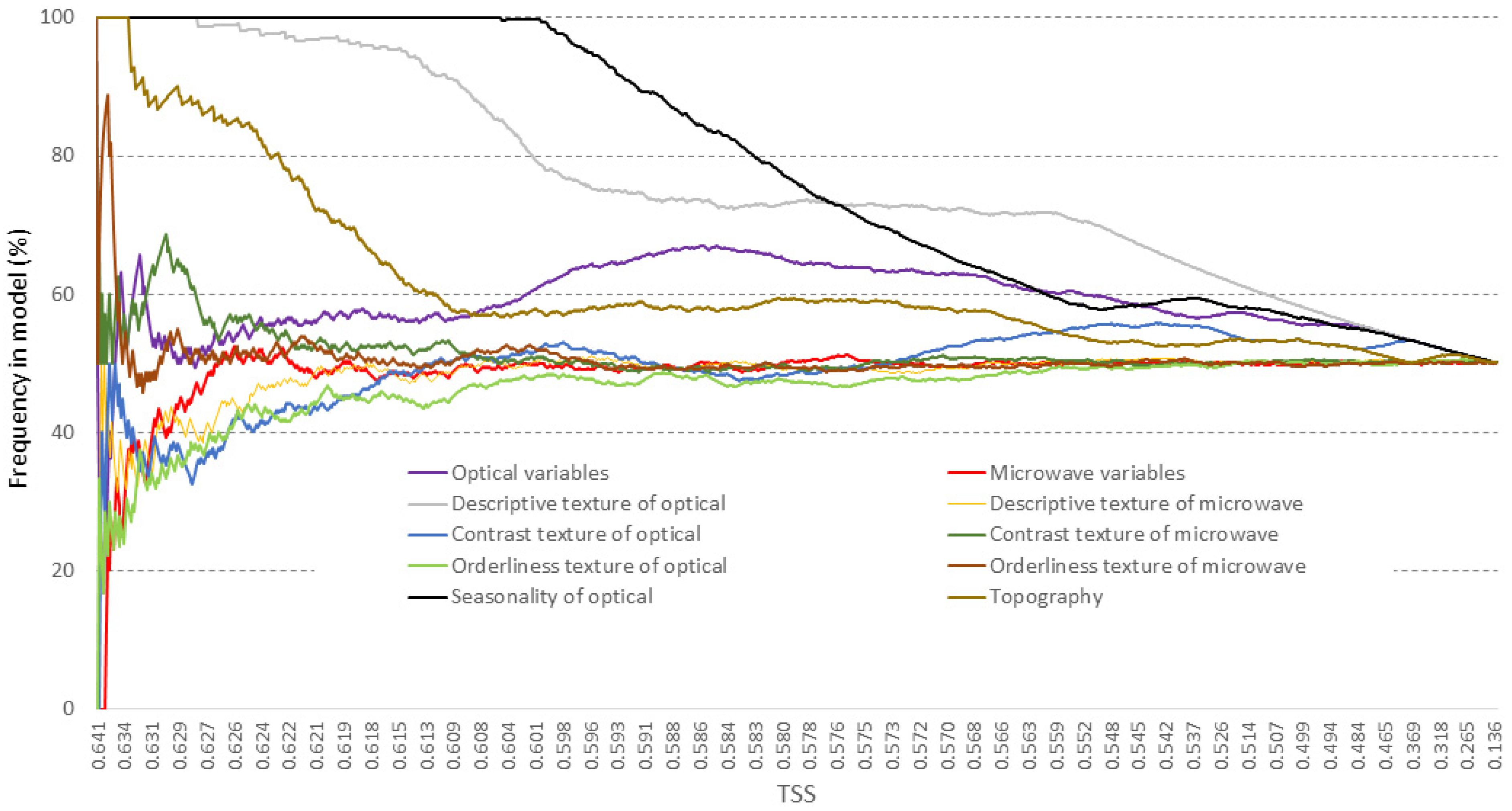
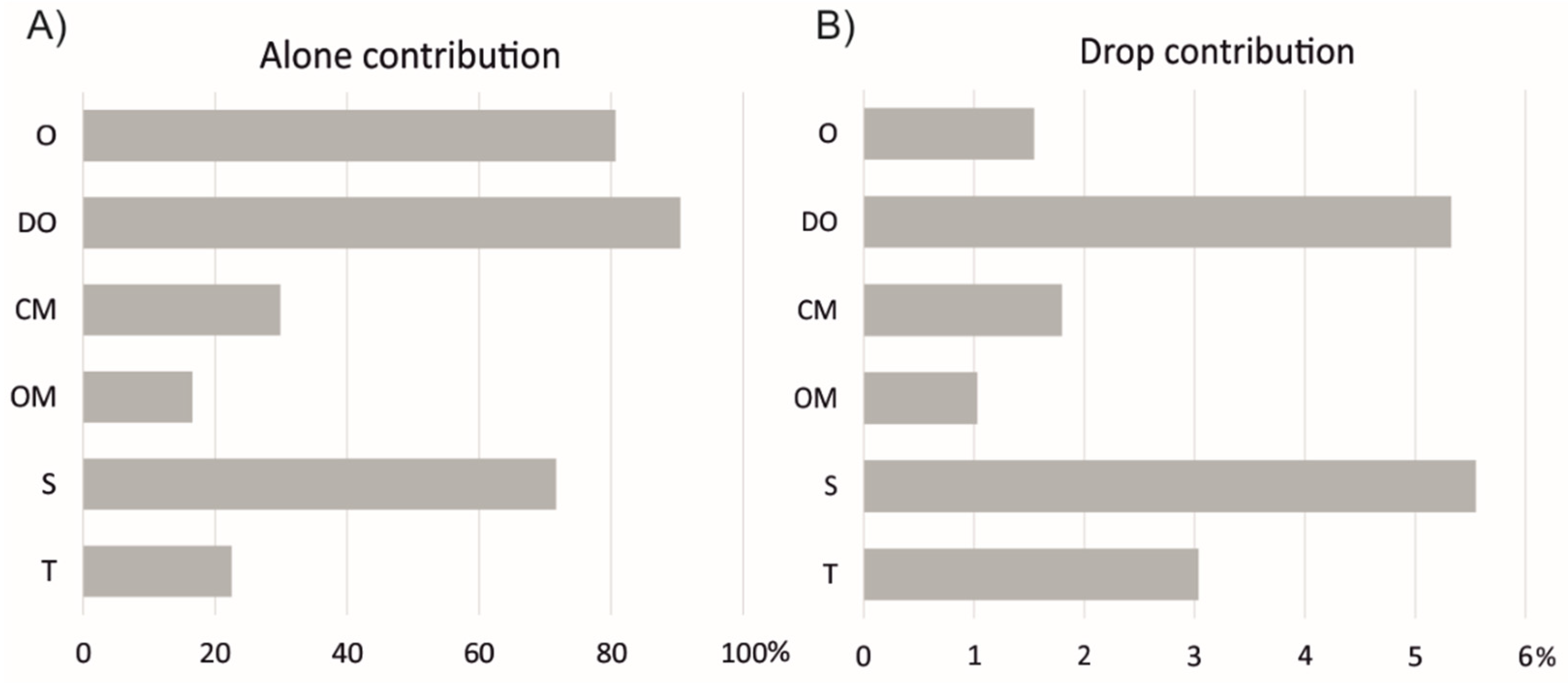
3.1. Variable Selection and Parameter Adjustment

The most frequent variable groups in the best performing models were seasonality, descriptive texture of optical, and topography (Figure 3). The best model (TSS 0.641) used six variable groups: Optical, descriptive texture of optical, contrast texture of microwave, orderliness texture of microwave, seasonality of optical, and topography. These variable groups showed different contributions in the best model. Descriptive texture of optical (90.5%), optical (80.6%), and seasonality (71.6%) showed the highest explanatory power based on alone contributions (Figure 4A), while seasonality (5.5%), descriptive texture of optical (5.3%), and topography (3.0%) had the highest importance in the drop contribution test (Figure 4B). The high and low contributions of optical group in alone and drop contributions test, respectively, indicated that the explanatory power of optical group overlapped with other variable group(s), and thus provided relatively minor added value to the final model. On the other hand, the low and relatively high contributions of topography group in alone and drop contributions test, respectively, indicated that the topography-related variables had poor explanatory power alone, but they bring significant value to the final model when combined with the other groups. Furthermore, the used microwave variable groups, descriptive texture of microwave and orderliness texture of microwave, had relatively modest alone and drop contributions.
The optimization of ntree and mtry parameters had minor effect on TSS (Supplementary Material, Figure S3). Highest TSS (0.647) was achieved with 3000 trees and 17 variables per node. However, the highest feasible result in terms of computation time was reached with 500 trees and 6 variables per node.

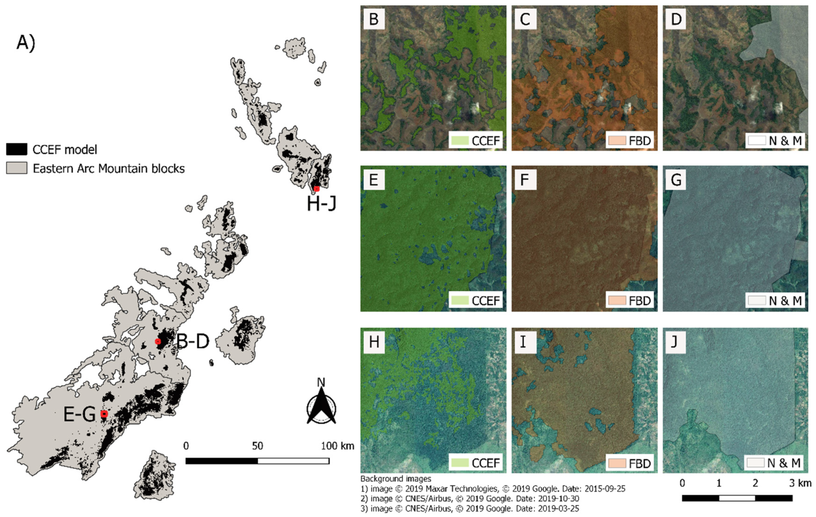
3.2. Coverage and Distribution of the Eastern Arc Forest

Based on CCEF model, approximately 296,000 ha of closed canopy natural forest remain in the EAM (Figure 5A and Table 2). The model area estimate for the whole EAM did not fit within error-adjusted area estimate calculated based on validation data indicating that the model was a conservative estimate of the remaining natural forests. Also, compared to the previous maps of EAF cover, CCEF model estimated less forest cover (Table 2). The overall accuracy (OA) of the CCEF model was 0.8 and TSS 0.57 tested with the independent validation data set. The accuracy of the CCEF model varied among the mountain blocks, being highest in Ukaguru and lowest in North Pare. In 10 out of 13 blocks, the CCEF model was the most accurate model compared to the previous forest maps from the EAM. Complete error matrices are reported in Supplementary Materials (Tables S4–S16).
The CCEF model captured the locations of small fragments and revealed the pattern of the remaining remnants effectively (Figure 5B–D). Moreover, the CCEF model identified the gaps of nonforested areas within the larger forest patches (Figure 5E–G). However, despite our multi-temporal and multi-sensor approach, some parts of CCEF model were still contaminated due to persistent cloud cover (Figure 5H–J).
The remaining EAFs were highly fragmented and isolated (Table 3). Approximately 23,500 ha (8%) of the forest area is in forest fragments smaller than 10 ha. East Usambara is spatially the most concise block with relatively small mean distances among forest patches and small standard deviation of the Euclidean distances. In Nguu, Ukaguru, and Rubeho, there exists multiple separate forest patch concentrations shown by relatively large mean patch size and high variation of distance between the patches. Mahenge is the most fragmented block with a high number of small size forest fragments.
The majority of the remaining EAF is protected (Table 3). However, the protection status varies among the blocks. In Malundwe, all of the forest areas are protected with IUCN, coded Mikumi National Park. Furthermore, in west and east Usambara over 70% of the forest is protected with IUCN-coded areas. On the other hand, in Uluguru over 80% of the forest is protected but only 1.3% of these areas are IUCN-coded and the rest of the forests are protected under national and village forest reserves. On average, the small remnants (<10 ha) are less protected. The most vulnerable blocks are Nguru and Mahenge where a vast majority of the forest is located outside the protected areas.
The CCEF model is freely available at Data Publisher for Earth & Environmental Science (PANGAEA) (https://doi.pangaea.de/10.1594/PANGAEA.914420).

4. Discussion

4.1. Extent, Fragmentation, and Protection of Eastern Arc Forests

The produced CCEF model showed that the EAF extent was lower than previous studies estimated, even though our study included the previously excluded small fragments (1–10 ha) [39,45]. The difference in the EAF coverage, compared to the previous estimations, is explained by the fact that the CCEF model identified the gaps of nonforested areas within the larger forest patches. Furthermore, the CCEF models improved the separation of closed canopy evergreen natural forests from other woody vegetation within the EAM including semideciduous woodlands, degraded forests, agroforests, and plantations. Furthermore, acknowledging the small fragments showed that the ecosystem is more fragmented, as previously considered. The number of fragments is over 30 times higher and the fragment size is one-third of the values reported previously [39]. However, on a positive side, the average distance from a fragment to the nearest fragment is less than previously reported.
Comparison of the CCEF model with the existing protected area network showed that some 24% is unprotected, confirming the previous estimates [43,47,52]. However, there are significant geographical differences in protected area coverage. Many previous studies on biodiversity values of the EAM have concentrated on the east and west Usambara, Uluguru, and Udzungwa, as these mountain blocks are considered most important for biodiversity [38]. In these mountain blocks, a vast majority of the forests are protected. However, in less-studied mountains of Nguru, Rubeho, or Mahenge [84] a vast majority of the forest remains unprotected.
In total, some 88% of forest patches less than 10 ha in size are unprotected. Although it is well known that significant conservation measures should be and have been targeted to the large forest fragments [39,82], there is a global tendency to underestimate the value of small fragments [19,46]. It is highly likely that many of the small fragments are holding significant extinction debt and their rehabilitation and connection to the larger fragments should be a priority. Therefore, we suggest that CCEF model should be used to evaluate and update the representativeness of the protected area network and target new inventories while acknowledging the limitations in available conservation resources.

4.2. Accuracy of the CCEF Model

Overall, the produced CCEF model had a moderate accuracy (TSS 0.57). The assessment was done with independent and statistically robust accuracy assessment following the state-of-the-art guidelines [85]. Since the confidence interval for the natural closed canopy forest did not include the value for the map area of CCEF model, the model can be considered a conservative estimate on the remaining EAFs. However, the discrepancy between the estimated area and map area was largely caused by the discrepancy of natural forest cover in Udzungwa. As the accuracy assessment of the previous forest estimates were based on expert opinion, our approach provided also a more robust assessment for previously mapped forest areas [39,45].
However, there were clear variations in model performance among EAM blocks, as shown by the TSS value range (0.36–0.87) (Table 2). The availability of cloud-free and temporally consistent data is a key prerequisite for developing a consistent model. In cloud-prone areas, the pixel-based median mosaic may be temporally inconsistent, as several images are needed to construct a cloud-free mosaic. This may have caused lower performance of the CCEF model in some blocks and can explain the discrepancy of area between the model and error-adjusted area estimate calculated based on validation samples. Furthermore, some clouds remained in the median mosaics, especially in the northern parts of the study area, leaving gaps in the CCEF model. As the Sentinel-2 image archives update, the availability of cloud-free images from the EAM will increase. Thus, updating the model every 2–3 years enables identification of the dynamics of EAFs and increases the reliability of the coverage.
The number of small fragments in the CCEF model was large and to some extent caused by the methodological approach. At some areas, natural closed canopy forests were found in patches surrounded by forests of sparser canopy cover. Such areas were found, e.g., in Mahenge and in Udzungwa scarp, where the forest cover is variating in terms of canopy cover and structure. In such areas, the CCEF model was only identifying the closed canopy patches, leading to a highly fragmented structure. These forest blocks showed also the highest discrepancies in forest area compared to Newmark and McNeally’s [39] work as they used human interpretation to define the forest borders. However, we argue that the spatial pattern of closed canopy forest patches is valuable information for conservation and management purposes. Future studies should concentrate on the forest disturbance dynamics within these areas and study the processes behind the sparser canopy cover areas.

4.3. Optimal Modelling Setup for Detecting Closed Canopy Natural Forests

The results of our study demonstrated that combining data from multiple sensors (optical, microwave) and of multiple natures (texture, topography, seasonality) improves the detection of closed canopy natural forests in a tropical environment. However, certain variable groups are clearly more valuable in increasing the model performance.
We found that texture metrics of Sentinel-2 imagery are highly meaningful predictors of closed canopy natural forest. This suggests that the heterogeneous texture of the natural forest canopy, caused by different age and height structures and different phenological phases of different species, can be identified with the texture metrics accounting for the neighborhood reflectance relationships. The importance of texture metrics has also been reported by other recent studies mapping forest types and species [33,70,86,87]. In addition to the texture, we found adding variables describing seasonality and topographical variance increases model performance, also reported by previous land cover classification studies [71,88,89]. In EAMs, many of the blocks are surrounded by deciduous woodlands with different temporal spectral signature compared to evergreen forests [38], which explains the importance of seasonality group in the model. Furthermore, as the EAFs locate at variating and rugged terrain, the hydrological conditions and solar radiation may vary substantially in small geographical areas [90], which explains the importance of topographical variables in the CCEF model.
Recent studies have shown that combining radar with optical data improves detection of tropical rainforests [88], mangrove forests [91], forest plantations [33], and upland vegetation [92], as well as forest attributes such as above-ground biomass or volume-growing stock [30,34,93]. Results of this study are in concordance with this knowledge as the best performing model included two microwave texture variable groups. However, their influence on the model’s performance was modest in both alone and drop contributions test. Furthermore, radar variables were not frequently present in the best models. Considering the tedious preprocessing of radar data, its use in similar studies should be carefully considered.
Bundling independent variables to groups caused certain limitations for assessing variables’ importance, though it was a necessity for computational reasons. Few variables, such as mean of texture and mean of seasonality, correlated with the band reflectance values [66] as they are simple descriptive statistical measures. Thus, these variables could have been grouped to multiple groups. The texture and seasonality groups, where these variables were eventually placed, had high average TSS and alone and drop contribution test results. However, it can be questioned if these groups would have had similar contribution on the model’s performance if these correlating variables had placed to Optical group instead. The grouping of the variables also limited the possibility to run standard statistical tests for variable importance due to the collinearity between the groups. Therefore, this study was only able to provide indicative guidance on the importance of the variable groups instead of full statistical evidence on independent variables.
On the modelling side, it is uncertain if 30 repetitions were enough to remove randomness caused by permutation from the averaged results. Alternative options could be repeated by random subsampling cross-validation with only a fraction of the observations used at each repetition or out-of-bag error estimates integrated to RF, though the reliability and independence of the latter is still debated [73,80]. Furthermore, in our case, modifying the RF model parameters ntree and mtry had negligible impact on model performance. The TSS variations were so minor that they could fit into the stochasticity caused by permutation. However, optimizing these parameters is an important step in the model development as their importance is context dependent [76].

4.4. Global Considerations

As is shown by this study, combining the advantages of multiple Earth observation sensors, machine learning approaches, and cloud computing has a significant potential to improve mapping of highly valuable fragmented evergreen forests. Previous studies have shown this potential in other key habitats, such as wetlands and heathlands [91,92,94,95].
Even though spatial information on most of the tropical forest ecosystems and GBHs exists, this information is often outdated and coarse [20,96,97,98]. Meanwhile, highly accurate baseline data are becoming a prerequisite for advanced Earth observation-based forest monitoring, such as detection of canopy disturbance and forest degradation [25] or in detailed ecological studies on the movements of those endangered species inhabiting these habitats, such as the primates of EAM [49]. Thus, there is a continuous need to improve the mapping of GBHs. We urge researchers and practitioners to consider the need to update the spatial information of other areas with outstanding biodiversity values.

5. Conclusions

This study demonstrated that recent developments in Earth observation regarding image availability, quality, and processing capacity, allow significant enhancements in mapping accuracies of fragmented tropical forests over large geographic areas. The results show that texture metrics of Sentinel-2 imagery, seasonality metrics derived from Landsat-8 time series, and topography metrics derived from SRTM DEM are highly meaningful predictors of closed canopy natural forest in the EAM of Tanzania and Kenya. Furthermore, texture metrics of Sentinel-1 imagery were found to improve the model performance slightly. The developed CCEF model shows that the coverage of the EAF is smaller than previously estimated, the remaining forests are more fragmented with 88% of the remnants being less than 10 ha in size, and that 24% of the natural forests are outside of a current conservation network. Therefore, the CCEF model facilitates evaluation and updates on the representativeness of the protected area network in this valuable GBH. The methodological setup was based on open source data and tools, providing a feasible approach for mapping and monitoring tropical forest remnants, especially relevant in the countries representing Global South where access to data and computing power has previously prohibited developing efficient and cost-effective approaches.

Supplementary Materials

The following are available online at https://www.mdpi.com/2072-4292/12/9/1429/s1, Table S1: Satellite imagery and ancillary geospatial data set used. Table S2: Training sample distribution based on tree cover and aspect. Table S3: Validation sample distribution to the EAF blocks. Table S4: Error matrix of Taita populated by the estimated proportion of area for each category. Table S5: Error matrix of North Pare. Table S6: Error matrix of South Pare. Table S7: Error matrix of West Usambara. Table S8: Error matrix of East Usambara. Table S9: Error matrix of Nguu. Table S10: Error matrix of Nguru. Table S11: Error matrix of Uluguru. Table S12: Error matrix of Ukaguru. Table S13: Error matrix of Rubeho. Table S14: Error matrix of Malundwe. Table S15: Error matrix of Mahenge. Table S16: Error matrix of Udzungwa. Figure S1: Spatial distribution of training samples. Figure S2: Spatial distribution of validation samples. Figure S3: TSS values of all the tested mtry and ntree combinations using the best variable group selection.

Author Contributions

Research design, J.K. and M.K.; data acquisition and preprocessing, J.K.; analysis, J.K. and M.K.; manuscript writing, J.K. and M.K.; manuscript comments N.K.; revision J.K.; supervision N.K. All authors have read and agreed to the published version of the manuscript.

Funding

The research was funded by the Academy of Finland (project: Sustainability, scale relations and structure-function-benefit chains in the landscape systems of the Tanzanian Southern Highlands (SUSLAND), 276126).

Acknowledgments

The authors wish to thank the University of Turku, Department of Geography and Geology and the University of Turku (UTU) Geospatial Labs (geospatial.utu.fi) for facilitating this research.

Conflicts of Interest

The authors declare no conflict of interest.

References

  1. Myers, N.; Mittermeier, R.A.; Mittermeier, C.G.; Da Fonseca, G.A.B.; Kent, J. Biodiversity hotspots for conservation priorities. Nature 2000, 403, 853–858. [Google Scholar] [CrossRef] [PubMed]
  2. Bradshaw, C.; Sodhi, N.; Peh, K.; Brook, B. Global evidence that deforestation amplifies flood risk and severity in the developing world. Glob. Chang. Biol. 2007, 13, 2379–2395. [Google Scholar] [CrossRef]
  3. Brinck, K.; Fischer, R.; Groeneveld, J.; Lehmann, S.; Dantas De Paula, M.; Pütz, S.; Sexton, J.O.; Song, D.; Huth, A. High resolution analysis of tropical forest fragmentation and its impact on the global carbon cycle. Nat. Commun. 2017, 8, 14855. [Google Scholar] [CrossRef] [PubMed] [Green Version]
  4. Brook, B.W.; Sodhi, N.S.; Bradshaw, C.J.A. Synergies among extinction drivers under global change. Trends Ecol. Evol. 2008, 23, 453–460. [Google Scholar] [CrossRef]
  5. Bellard, C.; Bertelsmeier, C.; Leadley, P.; Thuiller, W.; Courchamp, F. Impacts of climate change on the future of biodiversity. Ecol. Lett. 2012, 15, 365–377. [Google Scholar] [CrossRef] [Green Version]
  6. Garcia, R.A.; Cabeza, M.; Rahbek, C.; Araújo, M.B. Multiple Dimensions of Climate Change and Their Implications for Biodiversity. Science 2014, 344, 6183. [Google Scholar] [CrossRef] [Green Version]
  7. Cartwright, J. Ecological islands: Conserving biodiversity hotspots in a changing climate. Front. Ecol Environ. 2019, 17, 331–340. [Google Scholar] [CrossRef] [Green Version]
  8. Haddad, N.M.; Brudvig, L.A.; Clobert, J.; Davies, K.F.; Gonzalez, A.; Holt, R.D.; Lovejoy, T.E.; Sexton, J.O.; Austin, M.P.; Collins, C.D.; et al. Habitat fragmentation and its lasting impact on Earth’s ecosystems. Sci. Adv. 2015, 1, e1500052. [Google Scholar] [CrossRef] [Green Version]
  9. Taubert, F.; Fischer, R.; Groeneveld, J.; Lehmann, S.; Müller, M.S.; Rödig, E.; Wiegand, T.; Huth, A. Global patterns of tropical forest fragmentation. Nature 2018, 554, 519–522. [Google Scholar] [CrossRef]
  10. Ganivet, E.; Bloomberg, M. Towards rapid assessments of tree species diversity and structure in fragmented tropical forests: A review of perspectives offered by remotely sensed and field-based data. For. Ecol. Manag. 2019, 432, 40–53. [Google Scholar] [CrossRef]
  11. Mittermeier, R.A.; Turner, W.R.; Larsen, F.W.; Brooks, T.M.; Gascon, C. Global biodiversity conservation: The critical role of hotspots. In Biodiversity Hotspots–Distribution and Protection of Conservation Priority Areas; Zachos, F.E., Habel, J.C., Eds.; Springer: Berlin, Germany, 2011; pp. 3–22. [Google Scholar]
  12. Hrdina, A.; Romportl, D. Evaluating global biodiversity hotspots–Very rich and even more endangered. J. Landsc. Ecol. 2017, 10, 108–115. [Google Scholar] [CrossRef] [Green Version]
  13. Fahrig, L. Effects of habitat fragmentation on biodiversity. Annu. Rev. Ecol. Evol. Syst. 2003, 34, 487–515. [Google Scholar] [CrossRef] [Green Version]
  14. Decocq, G.; Andrieu, E.; Brunet, J.; Chabrerie, O.; De Frenne, P.; De Smedt, P.; Deconchat, M.; Diekmann, M.; Ehrmann, S.; Giffard, B.; et al. Ecosystem services from small forest patches in agricultural landscapes. Curr. For. Rep. 2016, 2, 30–44. [Google Scholar] [CrossRef] [Green Version]
  15. MacArthur, R.H.; Wilson, E.O. The Theory of Island Biogeography; Princeton University Press: Princeton, NJ, USA, 1967. [Google Scholar]
  16. Gibson, L.; Lynam, A.J.; Bradshaw, C.J.A.; He, F.; Bickford, D.P.; Woodruff, D.S.; Bumrungsri, S.; Laurance, W.F. Near-complete extinction of native small mammal fauna 25 years after forest fragmentation. Science 2013, 341, 1508–1510. [Google Scholar] [CrossRef]
  17. Pimm, S.L.; Brooks, T. Conservation: Forest Fragments, Facts, and Fallacies. Curr. Biol. 2014, 23, R1098–R1101. [Google Scholar] [CrossRef] [Green Version]
  18. Tulloch, A.I.T.; Barnes, M.D.; Ringma, J.; Fuller, R.A.; Watson, J.E.M. Understanding the importance of small patches of habitat for conservation. J. Appl. Ecol. 2016, 53, 418–429. [Google Scholar] [CrossRef] [Green Version]
  19. Wintle, B.A.; Kujala, H.; Whitehead, A.; Cameron, A.; Veloz, S.; Kukkala, A.; Moilanen, A.; Gordon, A.; Lentini, P.E.; Cadenhead, N.C.R.; et al. Global synthesis of conservation studies reveals the importance of small habitat patches for biodiversity. Proc. Natl. Acad. Sci. USA 2019, 116, 909–914. [Google Scholar] [CrossRef] [Green Version]
  20. Sloan, S.; Jenkins, C.N.; Joppa, L.N.; Gaveau, D.L.A.; Lawrence, W.F. Remaining natural vegetation in the global biodiversity hotspots. Biol. Conserv. 2014, 177, 12–24. [Google Scholar] [CrossRef]
  21. Hansen, M.C.; Potapov, P.V.; Moore, R.; Hancher, M.; Turubanova, S.A.; Tyukavina, A.; Thau, D.; Stehman, S.V.; Goetz, S.J.; Loveland, T.R.; et al. High-resolution global maps of 21st-century forest cover change. Science 2013, 342, 851–853. [Google Scholar] [CrossRef] [Green Version]
  22. Potapov, P.; Hansen, M.C.; Lastadius, L.; Turubanova, S.; Yaroshenko, A.; Thies, C.; Smith, W.; Zhuravleva, I.; Komarova, A.; Minnemeyer, S.; et al. The last frontiers of wilderness: Tracking loss of intact forest landscapes from 2017, 2000 to 2013. Sci. Adv. 2017, 3, e1600821. [Google Scholar] [CrossRef] [Green Version]
  23. Tuykavina, A.; Hansen, M.C.; Potapov, P.V.; Krylov, A.M.; Goetz, S.J. Pan-tropical hinterland forests: Mapping minimally disturbed forests. Glob. Ecol. Biogeogr. 2016, 25, 151–163. [Google Scholar] [CrossRef]
  24. Lechner, A.M.; Stein, A.; Jones, S.D.; Ferwerda, J.G. Remote sensing of small and linear features: Quantifying the effects of patch size and length, grid position and detectability on land cover mapping. Remote Sens. Environ. 2009, 113, 2194–2204. [Google Scholar] [CrossRef]
  25. Langner, A.; Miettinen, J.; Kukkonen, M.; Vancutsem, C.; Simonetti, D.; Vieilledent, G.; Verhegghen, A.; Gallego, J.; Stibig, H.-J. Towards Operational Monitoring of Forest Canopy Disturbance in Evergreen Rain Forests: A Test Case in Continental Southeast Asia. Remote Sens. 2018, 10, 544. [Google Scholar] [CrossRef] [Green Version]
  26. Lima, T.A.; Beuchle, R.; Lagner, A.; Grecchi, R.C.; Griess, V.C.; Achard, F. Comparing Sentinel-2 MSI and Landsat 8 OLI Imagery for Monitoring Selective Logging in the Brazilian Amazon. Remote Sens. 2019, 11, 961. [Google Scholar] [CrossRef] [Green Version]
  27. Laurin, G.V.; Puletti, N.; Hawthorne, W.; Liesenberg, V.; Corona, P.; Papale, D.; Chen, Q.; Valentini, R. Discrimination of tropical forest types, dominant species, and mapping of functional guilds by hyperspectral and simulated multispectral Sentinel-2 data. Remote Sens. Environ. 2016, 176, 163–176. [Google Scholar] [CrossRef] [Green Version]
  28. Banskota, A.; Kayastha, N.; Falkowski, M.J.; Wulder, M.A.; Froese, R.E.; White, J.C. Forest monitoring using landsat time series data: A review. Can. J. Remote Sens. 2014, 40, 362–384. [Google Scholar] [CrossRef]
  29. Laurin, G.V.; Balling, J.; Corona, P.; Mattioli, W.; Papale, D.; Puletti, N.; Rizzo, M.; Truckenbrodt, J.; Urban, M. Above-ground biomass prediction by sentinel-1 multitemporal data in central Italy with integration of alos2 and sentinel-2 data. J. Appl. Remote Sens. 2018, 12, 016008. [Google Scholar] [CrossRef]
  30. Vafaei, S.; Soosani, J.; Adeli, K.; Fadaei, H.; Naghavi, H.; Pham, T.D.; Bui, T.D. Improving accuracy estimation of forest aboveground biomass based on incorporation of alos-2 palsar-2 and sentinel-2a imagery and machine learning: A case study of the hyrcanian forest area (Iran). Remote Sens. 2018, 10, 172. [Google Scholar] [CrossRef] [Green Version]
  31. Marston, C.; Giraudoux, P. On the Synergistic Use of Optical and SAR Time-Series Satellite Data for Small Mammal Disease Host Mapping. Remote Sens. 2019, 11, 39. [Google Scholar] [CrossRef] [Green Version]
  32. Whyte, A.; Ferentinos, K.P.; Petropoulos, G.P. A new synergistic approach for monitoring wetlands using Sentinels-1 and 2 data with object-based machine learning algorithms. Environ. Model. Softw. 2018, 104, 40–54. [Google Scholar] [CrossRef] [Green Version]
  33. Torbick, N.; Ledoux, L.; Salas, W.; Zhao, M. Regional mapping of plantation extent using multisensor imagery. Remote Sens. 2016, 8, 236. [Google Scholar] [CrossRef] [Green Version]
  34. Ghosh, S.M.; Behera, M.D. Aboveground biomass estimation using multi-sensor data synergy and machine learning algorithms in a dense tropical forest. Appl. Geogr. 2018, 96, 29–40. [Google Scholar] [CrossRef]
  35. Gorelick, N.; Hancher, M.; Dixon, M.; Ilyushchenko, S.; Thau, D.; Moore, R. Google Earth Engine: Planetary-scale geospatial analysis for everyone. Remote Sens. Environ. 2017, 202, 18–27. [Google Scholar] [CrossRef]
  36. Schepaschenko, D.; See, L.; Lesiv, M.; Bastin, J.-F.; Mollicone, D.; Tsendbazar, N.E.; Bastin, L.; McCallum, I.; Laso Bayas, J.C.; Baklanov, A.; et al. Recent advances in forest observation with visual interpretation of very high-resolution imagery. Surv. Geophys. 2019, 40, 839–862. [Google Scholar] [CrossRef] [Green Version]
  37. Newmark, W.D. Forest Area, Fragmentation, and Loss in the Eastern Arc Mountains: Implications for the Conservation of Biological Diversity. J. East. Afr. Nat. Hist. 1998, 87, 29–36. [Google Scholar] [CrossRef]
  38. Burgess, N.D.; Butynski, T.M.; Cordeiro, N.J.; Doggart, N.H.; Fjeldsa, J.; Howell, K.M.; Kilahama, F.B.; Loader, S.P.; Lovett, J.C.; Mbilinyi, B.; et al. The biological importance of the Eastern Arc Mountains of Tanzania and Kenya. Biol. Conserv. 2007, 134, 209–231. [Google Scholar] [CrossRef]
  39. Newmark, W.D.; McNeally, P.B. Impact of habitat fragmentation on the spatial structure of the Eastern Arc forests in East Africa: Implications for biodiversity conservation. Biodivers. Conserv. 2018, 27, 1387–1402. [Google Scholar] [CrossRef]
  40. Balmford, A.; Moore, J.L.; Brooks, T.; Burgess, N.; Hansen, L.A.; Williams, P.; Rahbek, C. Conservation Conflicts Across Africa. Science 2001, 291, 2616–2619. [Google Scholar] [CrossRef]
  41. Brooks, T.M.; Mittermeier, R.A.; Mittermeier, C.G.; da Fonseca, G.A.; Rylands, A.B.; Konstant, W.R.; Flick, P.; Pilgrim, J.; Oldfield, S.; Magin, G.; et al. Habitat loss and extinction in the hotspots of biodiversity. Conserv. Biol. 2002, 16, 909–923. [Google Scholar] [CrossRef] [Green Version]
  42. Burgess, N.D.; Lovett, J.; Rodgers, A.; Kilahama, F.; Nashanda, E.; Davenport, T.; Butynski, T. Eastern Arc Mountains and Southern Rift. In Hotspots Revisited: Earth’s Biologically Richest and Most Endangered Ecoregions, 2nd ed.; Mittermeier, R.A., Robles-Gil, P., Hoffmann, M., Pilgrim, J.D., Brooks, T.M., Mittermeier, C.G., Lamoreux, J.L., Fonseca, G.A.B., Eds.; Cemex: San Pedro Garza, Mexico, 2004; pp. 245–255. [Google Scholar]
  43. Hall, J.; Burgess, N.D.; Lovett, J.; Mbilinyi, B.; Gereau, R.E. Conservation implications of deforestation across an elevational gradient in the Eastern Arc Mountains, Tanzania. Biol. Conserv. 2009, 142, 2510–2521. [Google Scholar] [CrossRef]
  44. Newmark, W.D. Conserving Biodiversity in East African forests: A study of the Eastern Arc Mountains. In Ecological Studies; Springer: Heidelberg, Germany, 2002; Volume 155, p. 195. [Google Scholar]
  45. Forestry and Beekeeping Division. Forest Area Baseline for the Eastern Arc Mountains; Mbilinyi, B.P., Malimbwi, R.E., Shemwetta, D.T.K., Songorwa, Zahabu, E., Katani, J.Z., Kashaigili, J., Eds.; For Conservation and Management of the Eastern Arc Mountain Forests; Forestry and Beekeeping Division: Dar es Salaam, Tanzania, 2006. [Google Scholar]
  46. Lindenmayer, D. Small patches make critical contributions to biodiversity conservation. Proc. Natl. Acad. Sci. USA 2019, 116, 717–719. [Google Scholar] [CrossRef] [PubMed] [Green Version]
  47. Platts, P.J.; Burgess, N.D.; Gereau, R.E.; Lovett, J.C.; Marshall, A.R.; McClean, C.J.; Pellikka, P.K.E.; Swetnam, R.D.; Marchant, R. Delimiting tropical mountain ecoregions for conservation. Environ. Conserv. 2011, 38, 312–332. [Google Scholar] [CrossRef] [Green Version]
  48. Lovett, J.C. Importance of the Eastern Arc Mountains for Vascular Plants. J. E. Afr. Nat. Hist. 1998, 87, 59–74. [Google Scholar] [CrossRef] [Green Version]
  49. Davenport, T.R.B.; Stanley, W.T.; Sargis, E.J.; De Luca, D.W.; Mpunga, N.E.; Machaga, S.J.; Olson, L.E. A new genus of African Monkey, Rungwecebus: Morphology, ecology, and molecular phylogenetics. Science 2006, 312, 1378–1381. [Google Scholar] [CrossRef] [PubMed] [Green Version]
  50. Rovero, F.; Marshall, A.R.; Jones, T.; Perkin, A. The primates of Udzungwa mountains: Diversity, ecology and conservation. J. Anthropol. Sci. 2009, 87, 93–126. [Google Scholar] [PubMed]
  51. Swetnam, R.D.; Fisher, B.; Mbilinyi, B.; Munishi, P.K.T.; Willcock, S.; Ricketts, T.; Mwakalila, S.; Balmford, A.; Burgess, N.D.; Marshall, A.R. Mapping socio-economic scenarios of land cover change: A GIS method to enable ecosystem service modelling. J. Environ. Manag. 2011, 92, 563–574. [Google Scholar] [CrossRef] [PubMed]
  52. Green, J.M.H.; Larrosa, C.; Burgess, N.D.; Balmford, A.; Johnston, A.; Mbilinyi, B.; Platts, P.J.; Coad, L. Deforestation in an African biodiversity hotspot: Extent, variation and the effectiveness of protected areas. Biol. Conserv. 2013, 164, 62–72. [Google Scholar] [CrossRef]
  53. Protected Planet, UNEP-WCMC and IUCN. The World Database on Protected Areas (WDPA) UNEP-WCMC and IUCN. 2019. Available online: www.protectedplanet.net (accessed on 12 December 2019).
  54. Drusch, M.; Del Bello, U.; Carlier, S.; Colin, O.; Fernandez, V.; Gascon, F.; Hoersch, B.; Isola, C.; Laberinti, P.; Martimort, P.; et al. Sentinel-2: ESA’s Optical High-Resolution Mission for GMES Operational Services. Remote Sens. Environ. 2012, 120, 25–36. [Google Scholar] [CrossRef]
  55. Kempeneers, P.; Soille, P. Optimizing Sentinel-2 image selection in a Big Data context. Big Earth Data 2017, 1, 145–148. [Google Scholar] [CrossRef]
  56. Martins, V.S.; Barbosa, C.C.F.; de Carvalho, L.A.S.; Jorge, D.S.F.; Lobo, F.D.L.; de Moraes Novo, E.M.L. Assessment of atmospheric correction methods for Sentinel-2 MSI images applied to Amazon floodplain lakes. Remote Sens. 2017, 9, 322. [Google Scholar] [CrossRef] [Green Version]
  57. Grabska, E.; Hostert, P.; Pflugmacher, D.; Ostapowicz, K. Forest Stand Species Mapping Using the Sentinel-2 Time Series. Remote Sens. 2019, 11, 1197. [Google Scholar] [CrossRef] [Green Version]
  58. Ottosen, T.-B.; Petch, G.; Hason, M.; Skjøth, C.A. Tree cover mapping based on Sentinel-2 images demonstrate high thematic accuracy in Europe. Int. J. Appl. Earth Obs. Geoinf. 2020, 84, 101947. [Google Scholar] [CrossRef]
  59. Torres, R.; Snoeij, P.; Geudtner, D.; Bibby, D.; Davidson, M.; Attema, E.; Potin, P.; Rommen, B.; Floury, N.; Brown, M. Gmes sentinel-1 mission. Remote Sens. Environ. 2012, 120, 9–24. [Google Scholar] [CrossRef]
  60. Dostálová, A.; Wagner, W.; Milenković, M.; Hollaus, M. Annual seasonality in Sentinel-1 signal for forest mapping and forest type classification. Int. J. Remote Sens. 2018, 39, 7738–7760. [Google Scholar] [CrossRef]
  61. SNAP-ESA Sentinel Application Platform v6.0. Available online: http://step.esa.int (accessed on 7 September 2018).
  62. Filipponi, F. Sentinel-1 GRD Preprocessing Workflow. Proceedings 2019, 18, 11. [Google Scholar] [CrossRef] [Green Version]
  63. Gómez, C.; White, J.C.; Wulder, M.A. Optical remotely sensed time series data for land cover classification: A review. ISPRS J. Photogramm. Remote Sens. 2016, 116, 55–72. [Google Scholar] [CrossRef] [Green Version]
  64. Jakubauskas, M.E.; Legates, D.R.; Kastens, J.H. Harmonic analysis of time-series AVHRR NDVI data. Photogramm. Eng. Remote Sens. 2001, 67, 461–470. [Google Scholar]
  65. Haralick, R.M.; Shanmugam, K.; Dinstein, I. Texture features for image classification. IEEE Trans. Syst. Man Cybern. 1973, 3, 610–621. [Google Scholar] [CrossRef] [Green Version]
  66. Hall-Beyer, M. Practical guidelines for choosing GLCM textures to use in landscape classification tasks over a range of moderate spatial scales. Int. J. Remote Sens. 2017, 38, 5. [Google Scholar] [CrossRef]
  67. Sesnie, S.E.; Gessler, P.E.; Finegan, B.; Thessler, S. Integrating Landsat TM and SRTM-DEM derived variables with decision trees for habitat classification and change detection in complex neotropical environments. Remote Sens. Environ. 2008, 112, 2145–2159. [Google Scholar] [CrossRef]
  68. Sexton, J.O.; Song, X.-P.; Feng, M.; Noojipady, P.; Anand, A.; Huang, C.; Kim, D.-H.; Collins, K.M.; Channan, S.; DiMiceli, C.; et al. Global, 30-m resolution continuous fields of tree cover: Landsat-based rescaling of MODIS vegetation continuous fields with lidar-based estimates of error. Int. J. Dig. Earth 2013, 6, 427–448. [Google Scholar] [CrossRef] [Green Version]
  69. Jarvis, A.; Reuter, H.I.; Nelson, A.; Guevara, E. Hole-Filled Seamless SRTM Data (Online) V4. International Centre for Tropical Agriculture (CIAT). 2008. Available online: http://srtm.csi.cgiar.org (accessed on 7 January 2019).
  70. Saah, D.; Johnson, G.; Ashmall, B.; Tondapu, G.; Tenneson, K.; Patterson, M.; Poortinga, A.; Markert, K.; Quyen, N.H.; San Aung, K.; et al. Collect Earth: An online tool for systematic reference data collection in land cover and use applications. Environ. Model. Softw. 2019, 118, 166–171. [Google Scholar] [CrossRef]
  71. Dong, J.; Xiao, X.; Chen, B.; Torbick, N.; Jin, C.; Zhang, G.; Biradar, C. Mapping deciduous rubber plantations through integration of PALSAR and multitemporal Landsat imagery. Remote Sens. Environ. 2013, 134, 392–402. [Google Scholar] [CrossRef]
  72. Koskinen, J.; Leinonen, U.; Vollrath, A.; Ortmann, A.; Lindquist, E.; d’Annunzio, R.; Pekkarinen, A.; Käyhkö, N. Participatory mapping of forest plantations with Open Foris and Google Earth Engine. ISPRS J. Photogramm. Remote Sens. 2019, 148, 63–74. [Google Scholar] [CrossRef]
  73. Rodriguez-Galiano, V.F.; Ghimire, B.; Rogan, J.; Chica-Olmo, M.J.; Rigol-Sanchez, P. An assessment of the effectiveness of a random forest classifier for land-cover classification. ISPRS J. Photogramm. Remote Sens. 2012, 67, 93–104. [Google Scholar] [CrossRef]
  74. Belgiu, M.; Drăguţ, L. Random forest in remote sensing: A review of applications and future directions. ISPRS J. Photogramm. Remote Sens. 2016, 114, 24–31. [Google Scholar] [CrossRef]
  75. Breiman, L. Random forests. Mach. Learn. 2001, 45, 5–32. [Google Scholar] [CrossRef] [Green Version]
  76. Mutanga, O.; Adam, E.; Cho, M.A. High density biomass estimation for wetland vegetation using WorldView-2 imagery and random forest regression algorithm. Int. J. Appl. Earth Obs. Geoinf. 2012, 18, 399–406. [Google Scholar] [CrossRef]
  77. Allouche, O.; Tsoar, A.; Kadmon, R. Assessing the accuracy of species distribution models: Prevalence, kappa and true skill statistic (TSS). J. Appl. Ecol. 2006, 43, 1223–1232. [Google Scholar] [CrossRef]
  78. Landis, J.R.; Koch, G.G. The Measurement of Observer Agreement for Categorical Data. Biometrics 1977, 33, 159–174. [Google Scholar] [CrossRef] [Green Version]
  79. Lusk, C.H.; McGlone, M.S.; Overton, J.M. Climate predicts the proportion of divaricate plant species in New Zealand arborescent assemblages. J. Biogeogr. 2016, 43, 1881–1892. [Google Scholar] [CrossRef]
  80. Kukkonen, M.O.; Muhammad, M.J.; Käyhkö, N.; Luoto, M. Urban expansion in Zanzibar City, Tanzania: Analyzing quantity, spatial patterns and effects of alternative planning approaches. Land Use Policy 2018, 71, 554–565. [Google Scholar] [CrossRef]
  81. Korfanta, N.; Newmark, W.D.; Kaufman, M.J. Long-term demographic consequences of habitat fragmentation to a tropical understory bird community. Ecology 2012, 93, 2548–2559. [Google Scholar] [CrossRef] [PubMed]
  82. Cordeiro, N.J.; Borghesio, L.; Joho, M.P.; Monoski, T.J.; Mkongewa, V.J.; Dampf, C.J. Forest fragmentation in an African biodiversity hotspot impacts mixed-species bird flocks. Biol. Conserv. 2015, 188, 61–71. [Google Scholar] [CrossRef] [Green Version]
  83. McGarigal, K.; Cushman, S.A.; Ene, E. FRAGSTATS v4: Spatial Pattern Analysis Program for Categorical and Continuous Maps. Computer Software Program Produced by the Authors at the University of Massachusetts, Amherst. 2012. Available online: http://www.umass.edu/landeco/research/fragstats/fragstats.html (accessed on 20 September 2019).
  84. Doggart, N.; Perkin, A.; Kiure, J.; Fjeldså, J.; Poynton, J.; Burgess, N. Changing places: How the results of new field work in the Rubeho Mountains influence conservation priorities in the Eastern Arc Mountains of Tanzania. Afr. J. Ecol. 2006, 44, 134–144. [Google Scholar] [CrossRef]
  85. Olofsson, P.; Foody, G.M.; Herold, M.; Stehman, S.V.; Woodcock, C.E.; Wulder, M.A. Good practices for estimating area and assessing accuracy of land change. Remote Sens. Environ. 2014, 148, 42–57. [Google Scholar] [CrossRef]
  86. Lu, D.; Li, G.; Moran, E.; Dutra, E.; Batistella, M. The roles of textural images in improving land-cover classification in the Brazilian Amazon. Int. J. Remote Sens. 2014, 35, 24. [Google Scholar] [CrossRef] [Green Version]
  87. Erinjery, J.J.; Singh, M.; Kent, R. Mapping and assessment of vegetation types in the tropical rainforests of the Western Ghats using multispectral Sentinel-2 and SAR Sentinel-1 satellite imagery. Remote Sens. Environ. 2018, 216, 345–354. [Google Scholar] [CrossRef]
  88. Jin, Y.; Liu, X.; Chen, Y.; Liang, X. Land-cover mapping using Random Forest classification and incorporating NDVI time-series and texture: A case study of central Shandong. Int. J. Remote Sens. 2018, 39, 23. [Google Scholar] [CrossRef]
  89. Chiang, S.-H.; Valdez, M. Tree Species Classification by Integrating Satellite Imagery and Topographic Variables Using Maximum Entropy Method in a Mongolian Forest. Forests 2019, 10, 961. [Google Scholar] [CrossRef] [Green Version]
  90. Aguilar, C.; Herrero, J.; Polo, M. Topographic effects on solar radiation distribution in mountainous watersheds and their influence on reference evapotranspiration estimates at watershed scale. Hydrol. Earth Syst. Sci. 2010, 14, 2479–2494. [Google Scholar] [CrossRef] [Green Version]
  91. Crowson, M.; Warren-Thomas, E.; Hill, J.K.; Hariyadi, B.; Agu, F.; Saad, A.; Hamer, K.C.; Hodgson, J.A.; Kartika, W.D.; Lucey, J.; et al. A comparison of satellite remote sensing data fusion methods to map peat swamp forest loss in Sumatra, Indonesia. Remote Sens. Ecol. Conserv. 2018, 5, 247–258. [Google Scholar] [CrossRef] [Green Version]
  92. Barrett, B.; Raab, C.; Cawkwell, F.; Green, S. Upland vegetation mapping using Random Forests with optical and radar satellite data. Remote Sens. Ecol. Conserv. 2016, 2, 212–231. [Google Scholar] [CrossRef] [PubMed]
  93. Mauya, E.W.; Koskinen, J.; Tegel, K.; Hämäläinen, J.; Kauranne, T.; Käyhkö, N. Modelling and Predicting the Growing Stock Volume in Small-Scale Plantation Forests of Tanzania Using Multi-Sensor Image Synergy. Forests 2019, 10, 279. [Google Scholar] [CrossRef] [Green Version]
  94. Corbane, C.; Lang, S.; Pipkins, K.; Alleaume, S.; Deshayes, M.; Millán, V.E.G.; Strasser, T.; Borre, J.V.; Toon, S.; Förster, M. Remote sensing for mapping natural habitats and their conservation status−New opportunities and challenges. Int. J. Appl. Earth Obs. Geoinf. 2015, 37, 7–16. [Google Scholar] [CrossRef]
  95. Schmidt, J.; Fassnacht, F.E.; Forster, M.; Schmidtlein, S. Synergetic use of Sentinel-1 and Sentinel-2 for assessments of heathland conservation status. Remote Sens. Ecol. Conserv. 2018, 4, 225–239. [Google Scholar] [CrossRef] [Green Version]
  96. Harris, G.M.; Jenkins, C.N.; Pimm, S.L. Refining biodiversity conservation priorities. Conserv. Biol. 2005, 19, 1957–1968. [Google Scholar] [CrossRef]
  97. Murray-Smith, C.; Brummitt, N.A.; Oliveira-Filho, A.T.; Bachman, S.; Moat, J.; Lughadha, E.M.N.; Lucas, E.J. Plant diversity hotspots in the Atlantic Coastal Forests of Brazil. Conserv. Biol. 2009, 23, 151–163. [Google Scholar] [CrossRef]
  98. Noroozi, J.; Talebi, A.; Doostmohammadi, M.; Rumpf, S.B.; Linder, H.P.; Schneeweiss, G.M. Hotspots within a global biodiversity hotspot-areas of endemism are associated with high mountain ranges. Sci. Rep. 2018, 8, 10345. [Google Scholar] [CrossRef] [Green Version]
Figure 1. Eastern Arc Mountains consist of 13 blocks located in Tanzania and Kenya [47].
Remotesensing 12 01429 g001
Figure 2. Illustration of methodological design and its six phases. In phase 1, GRD (ground range detected), GLCM (gray-level co-occurrence matrix), and NDVI (normalized difference vegetation index). In phase 4, ntree (number of trees) and mtry (number of variables per node). In phase 5, CCEF (closed canopy evergreen natural forest). In phase 6, ENN (Euclidean nearest neighbor) distance and WDPA (World Database of Protected Areas).
Remotesensing 12 01429 g002
Figure 3. Frequency of variable groups used in the 1023 models ranked against the True Skill Statistic (TSS). Each variable group was used in 512 models and, thus, the frequency of each variable group converged to 50% when all models were considered. Seasonality, descriptive texture of optical, and topography were most frequently used in the best models (highest TSS) while microwave variables, orderliness, and contrast texture of optical groups were less frequent in the best models. All the models were built with default parameters (ntree = 500, mtry n/3).
Remotesensing 12 01429 g003
Figure 4. Alone (A) and drop (B) contributions of the variable groups in the best model proportioned against the TSS. O (optical), DO (descriptive texture of optical), CM (contrast texture of microwave), OM (orderliness texture of microwave), S (seasonality), and T (topography).
Remotesensing 12 01429 g004
Figure 5. Highlighted features of CCEF model (A) compared with the forest map of Forestry and Beekeebing Division (FBD) [45] (center), and Newmark and McNeally [39] (right) in 1:80,000 scale. Figures (BD) illustrate the potential of the products for accurate small forest fragment detection, figures (EG) illustrate the potential to detect gaps of open or sparsely forested areas within large fragments, and figures (HJ) illustrate the gaps in the CCEF model caused by persistent cloud cover.
Remotesensing 12 01429 g005
Table 1. Variable groups, variables within group, and number of variables in each group.
GroupVariables within GroupNumber of Variables
Optical variablesSentinel-2 bands (B2–B8A, B11–B12)10
Microwave variablesSentinel-1 bands (VH, VV)2
Descriptive texture of opticalDescriptive group haralicks (mean, variance, correlation) of Sentinel-2 bands30
Descriptive texture of microwaveDescriptive group haralicks (mean, variance, correlation) of Sentinel-1 bands6
Contrast texture of opticalContrast group haralicks (contrast, dissimilarity, homogeneity) of Sentinel-2 bands30
Contrast texture of microwaveContrast group haralicks (contrast, dissimilarity, homogeneity) of Sentinel-1 bands6
Orderliness texture of opticalOrderliness group haralicks (energy, entropy) of Sentinel-2 bands20
Orderliness texture of microwaveOrderliness group haralicks (energy, entropy) of Sentinel-1 bands4
Seasonality of opticalSeasonality of Landsat-8 derived NDVI (magnitude, phase, mean, std)4
TopographyTopography (altitude, slope, aspect)3
Table 2. Area estimates and accuracy of forest maps of the Eastern Arc Mountain (EAM) blocks evaluated based on independent validation data.
CCEF ModelFBD [45]Newmark and McNeally [39]
Estimated Area (ha)Map Area (ha)Map OAMap TSSMap Area (ha)Map OAMap TSSMap Area (ha)Map OAMap TSS
Taita607 ± 736230.760.36---5900.760.34
North Pare2287 ± 29526480.70.3927000.80.5915460.80.61
South Pare11,174 ± 83410,9420.870.7213,8000.750.3411,3800.780.47
West Usambara23,116 ± 135223,5780.830.6231,9000.660.1728,2130.760.39
East Usambara25,995 ± 160321,7790.720.5526,3000.590.0930,1100.860.57
Nguu12,472 ± 76611,7990.890.8218,8000.690.2316,1700.780.48
Nguru21,897 ± 134022,6660.840.6329,7000.690.2329,9270.730.28
Uluguru22,704 ± 129125,2430.830.5626,6980.740.3825,9630.870.68
Ukaguru12,993 ± 67813,7000.930.8717,2710.60.0117,7420.80.50
Rubeho35,212 ± 151932,3940.880.7347,1310.690.2142,2740.760.38
Malundwe803 ± 683440.90.771740.520.1811410.580
Mahenge11,789 ± 123511,2140.770.4819180.420.1754740.3−0.38
Udzungwa150,254 ± 5000119,2790.750.50135,2760.60.20195,3210.660.20
Total333,978 ± 5621296,2090.80.57351,6680.630.21405,8510.720.41
Table 3. Fragmentation and isolation metrics and protection estimation status of the Eastern Arc forests.
Fragmentation and IsolationProtection Status
Num.of Patches Num.of Patches (<10 ha)Forest Area (<10 ha) (%)ENN Mean (m)ENN StD (m)Mean Forest Patch Area (ha)Small Forest Patches (1–10 ha) Unprotected (%)Forests Unprotected (%)Forest Protected with IUCN (%)Forests Protected (%)
Taita645826.822447710100100--
North Pare92747268486296641.153.958.9
South Pare2261955.1260569486213.4386.6
West Usambara4113423.9191507576323.375.676.7
East Usambara4914334.9120170445327.872.272.2
Nguu1671473.54161683713513.370.886.7
Nguru2982622.8199298769277.721.822.3
Uluguru7326916.5204463348719.31.180.7
Ukaguru1771523371895777915.631.884.4
Rubeho570496425079757353854.762
Malundwe292822.91712721200100100
Mahenge156914463320435179789.50.210.5
Udzungwa525947399.8190-22196.444.893.6
Total/Mean10,08590637.7203581298823.942.176.1
ENN = Euclidean nearest neighbor distance.

