Lake Ice-Water Classification of RADARSAT-2 Images by Integrating IRGS Segmentation with Pixel-Based Random Forest Labeling


Abstract
1. Introduction
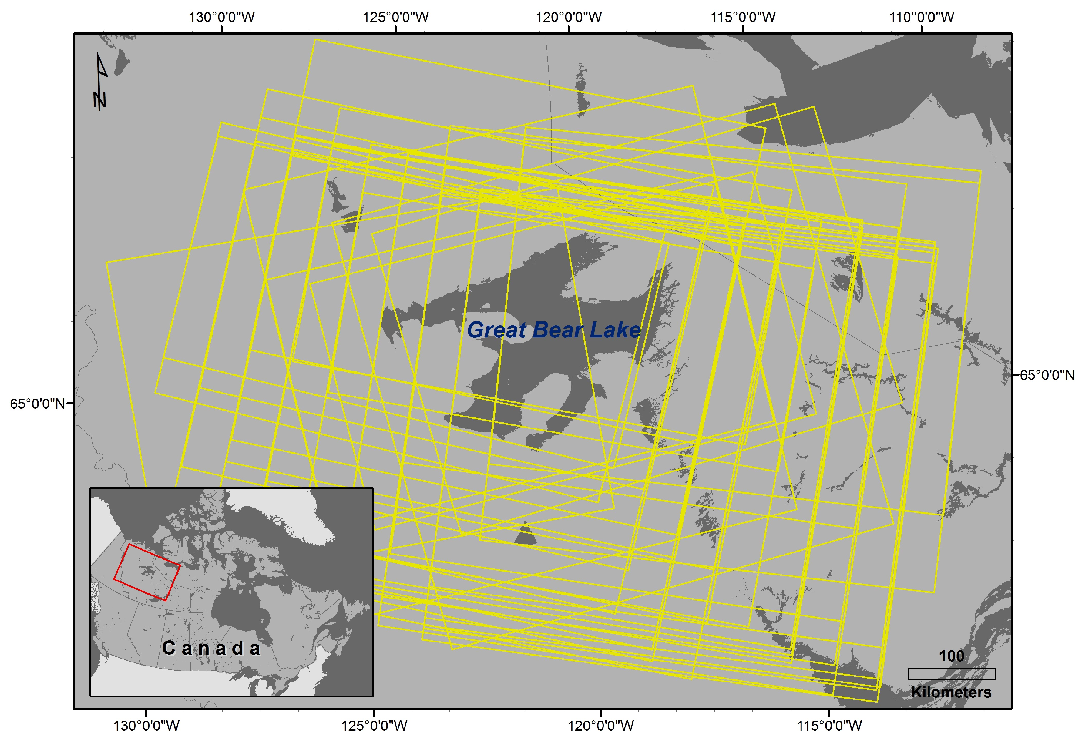
2. Data
2.1. Synthetic Aperture Radar Data
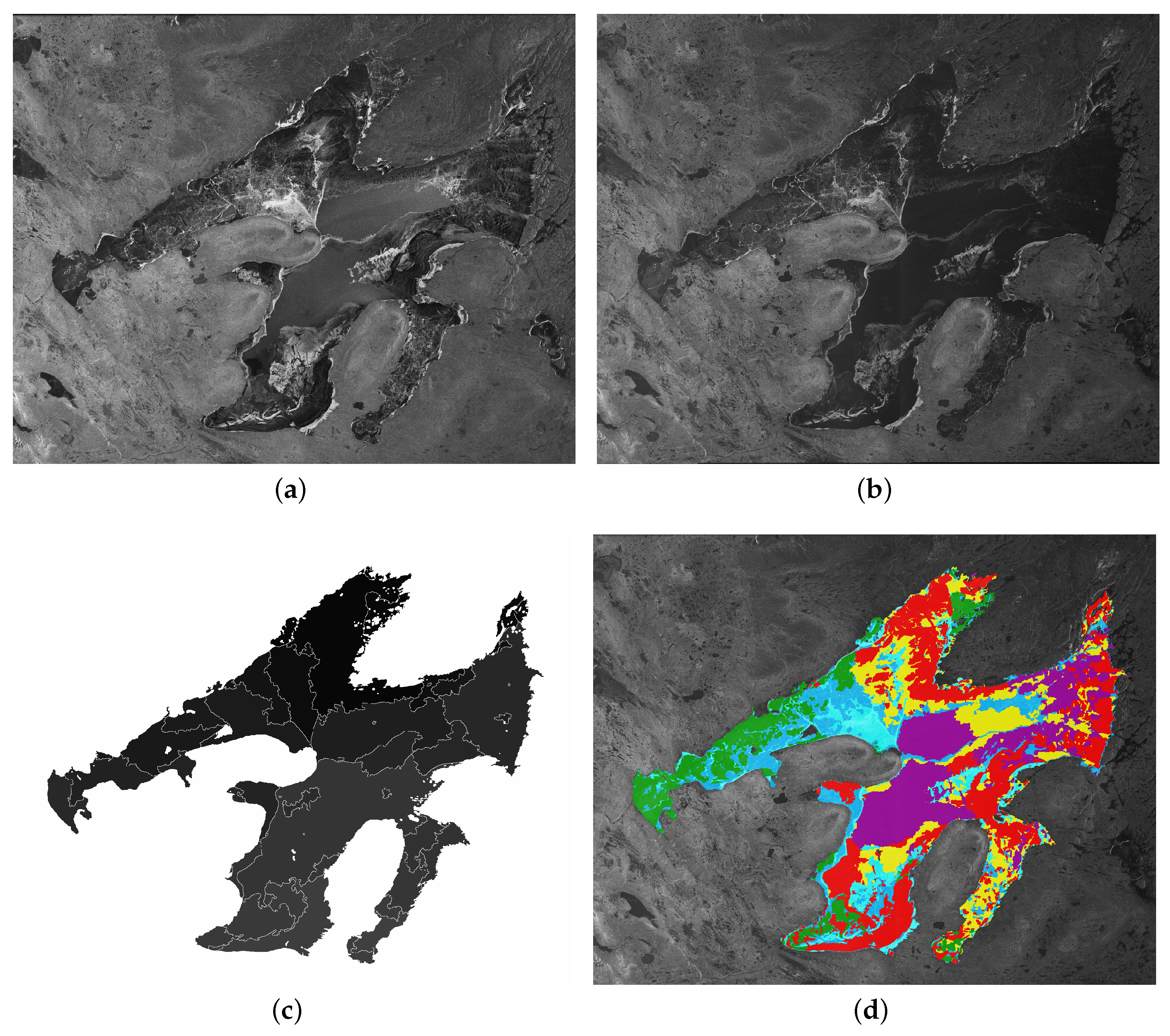
2.2. Reference Data
3. Methodology
3.1. IRGS Segmentation
3.2. IRGS-Manual Semi-Automated Classification
3.3. Automated Classification
3.3.1. Features
- Contrast Group: contrast (CON), dissimilarity (DIS), homogeneity (HOM)
- Orderliness Group: applied second moment (ASM), entropy (ENT), inverse moment (INV)
- Statistics Group: mean (MU), standard deviation (STD), correlation (COR)
3.3.2. Classifiers
Support Vector Machine
Random Forest
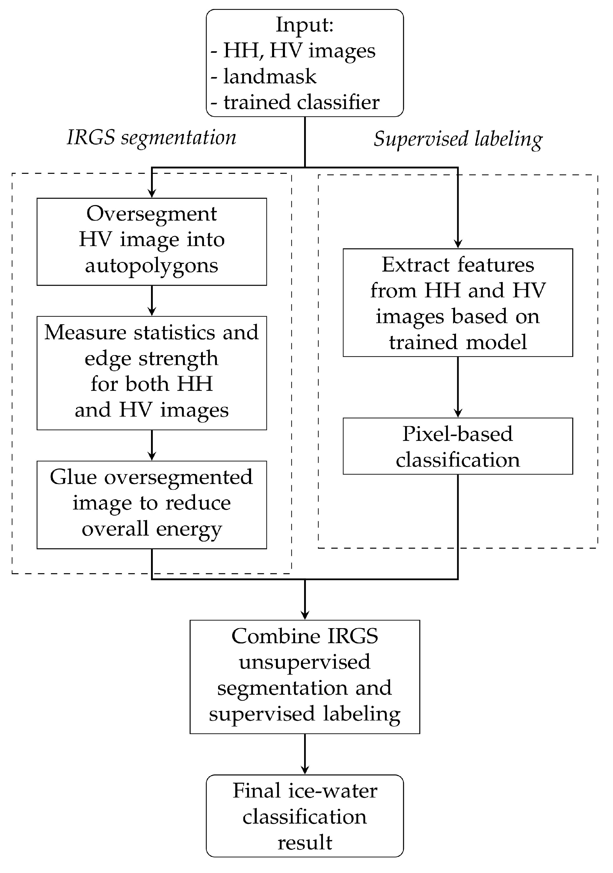
3.4. Integration of Segmentation and Labeling
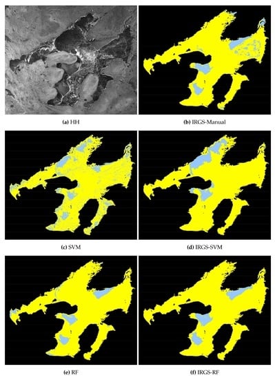
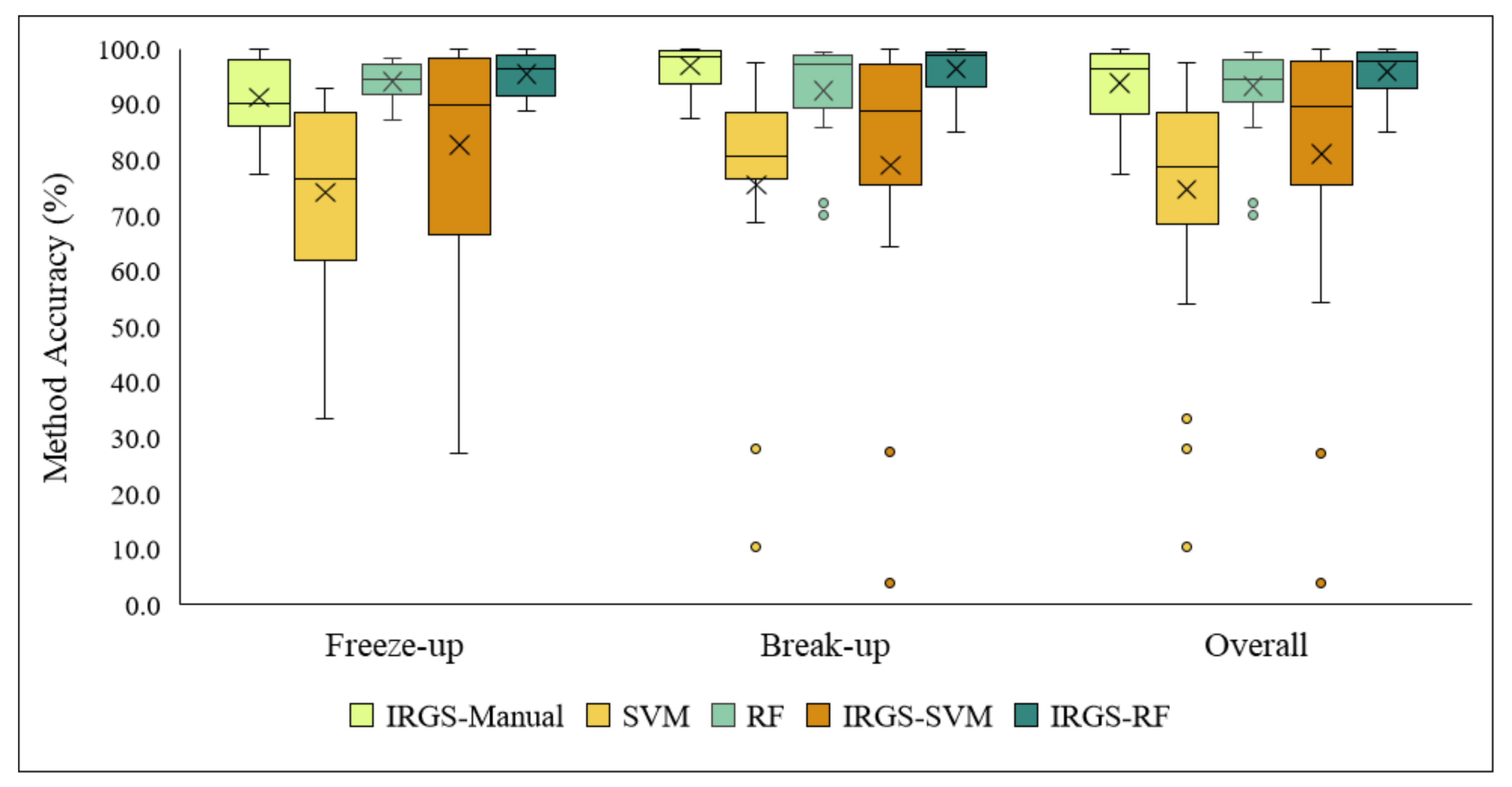
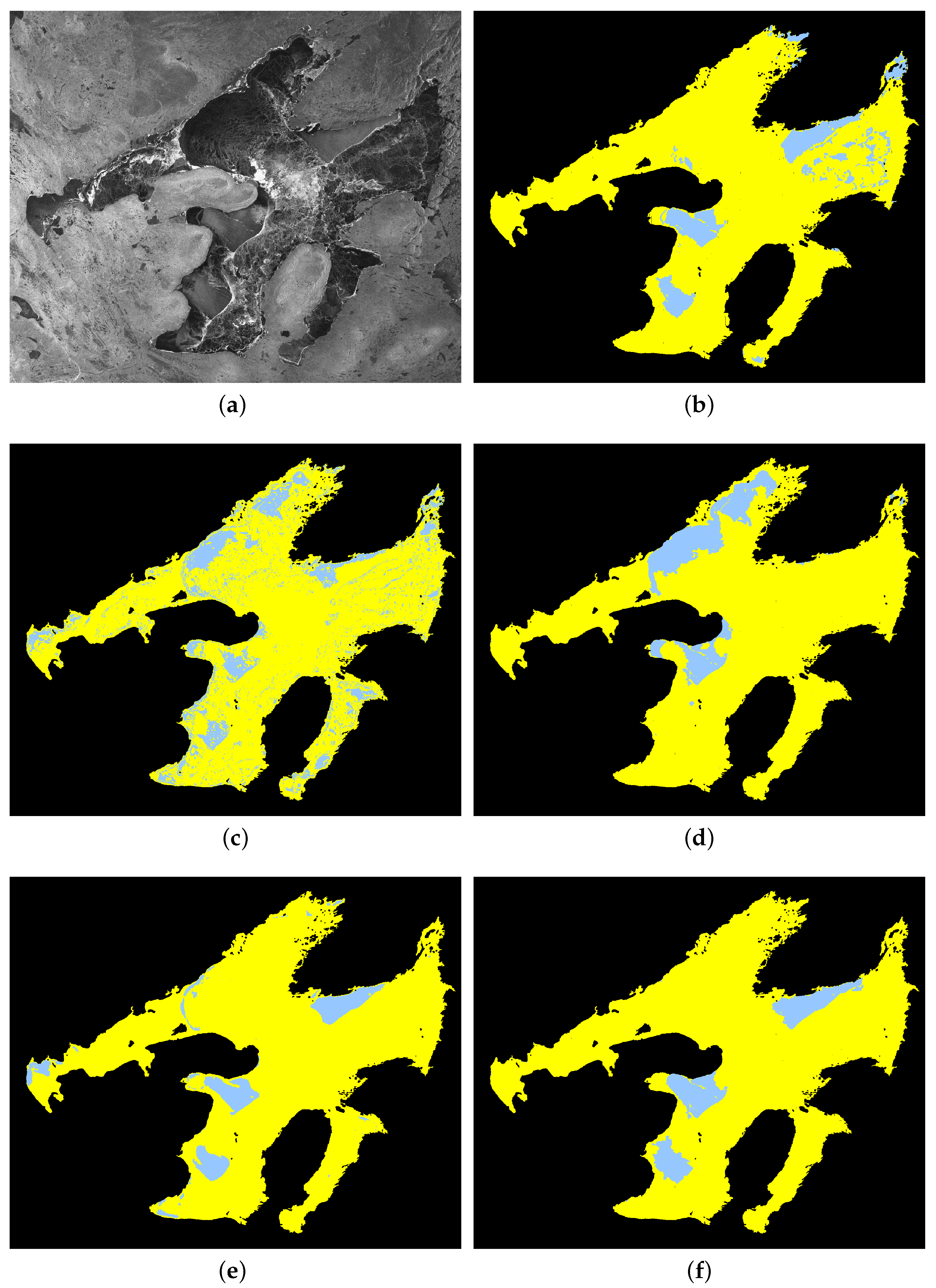
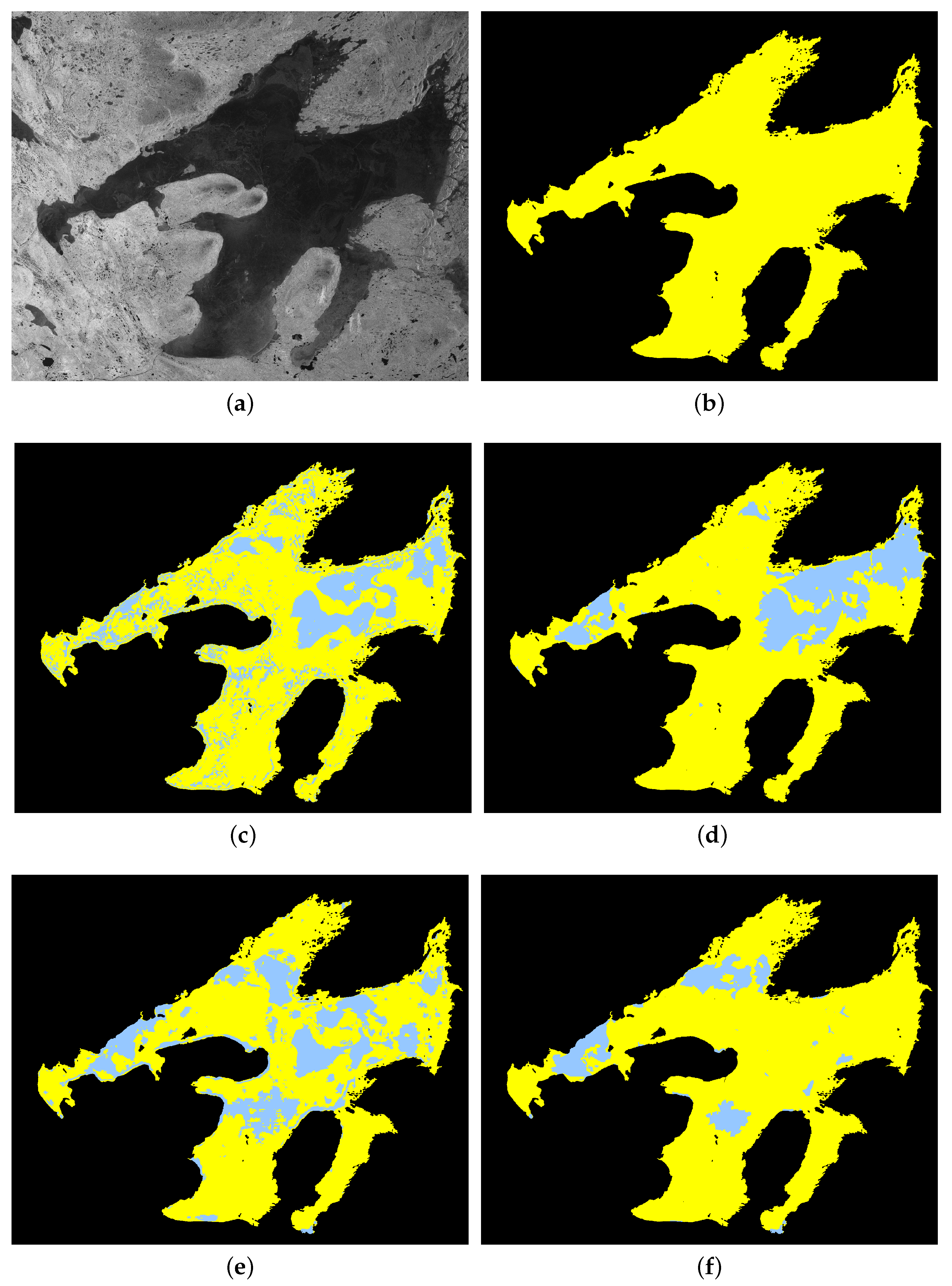
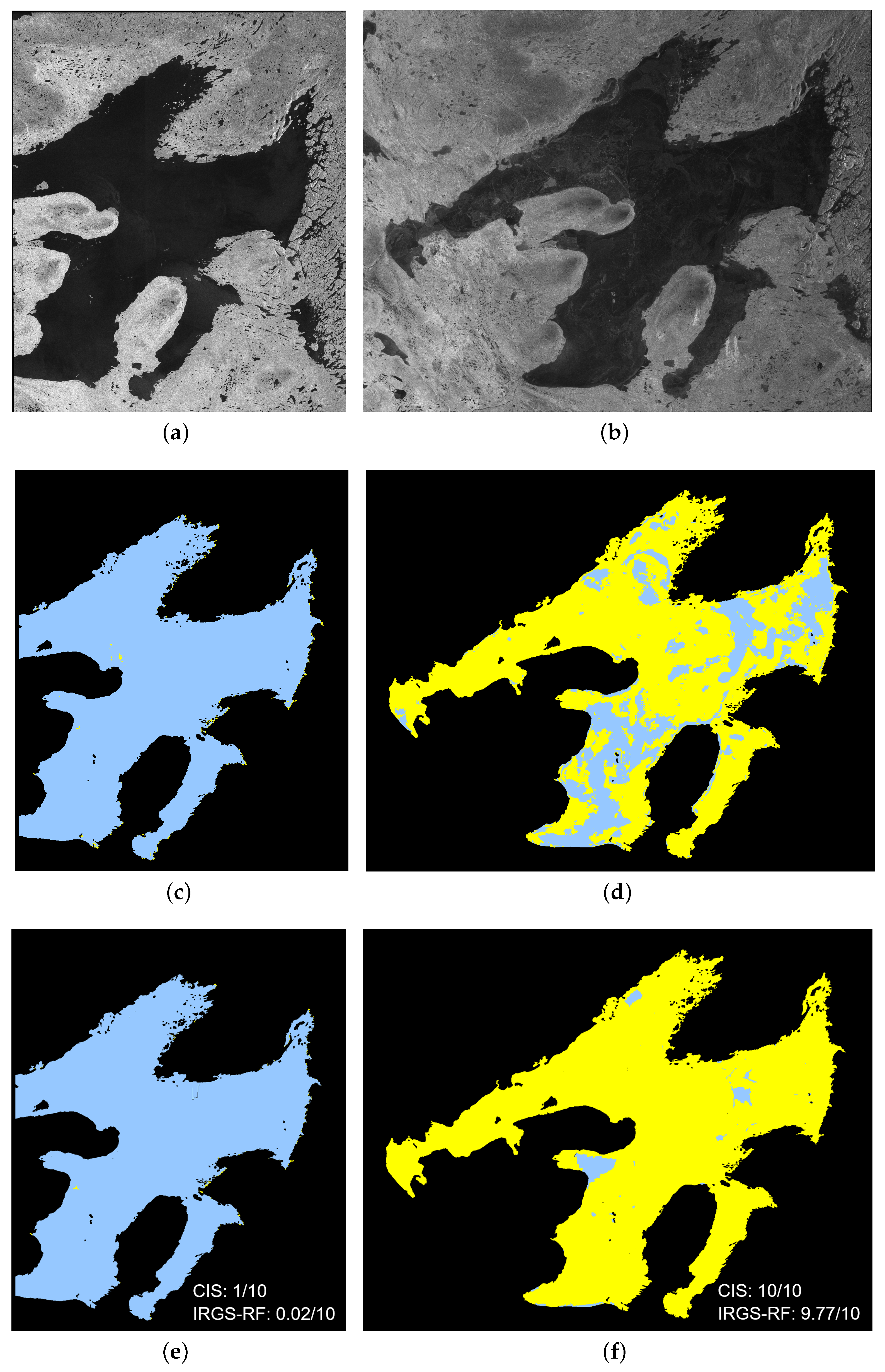
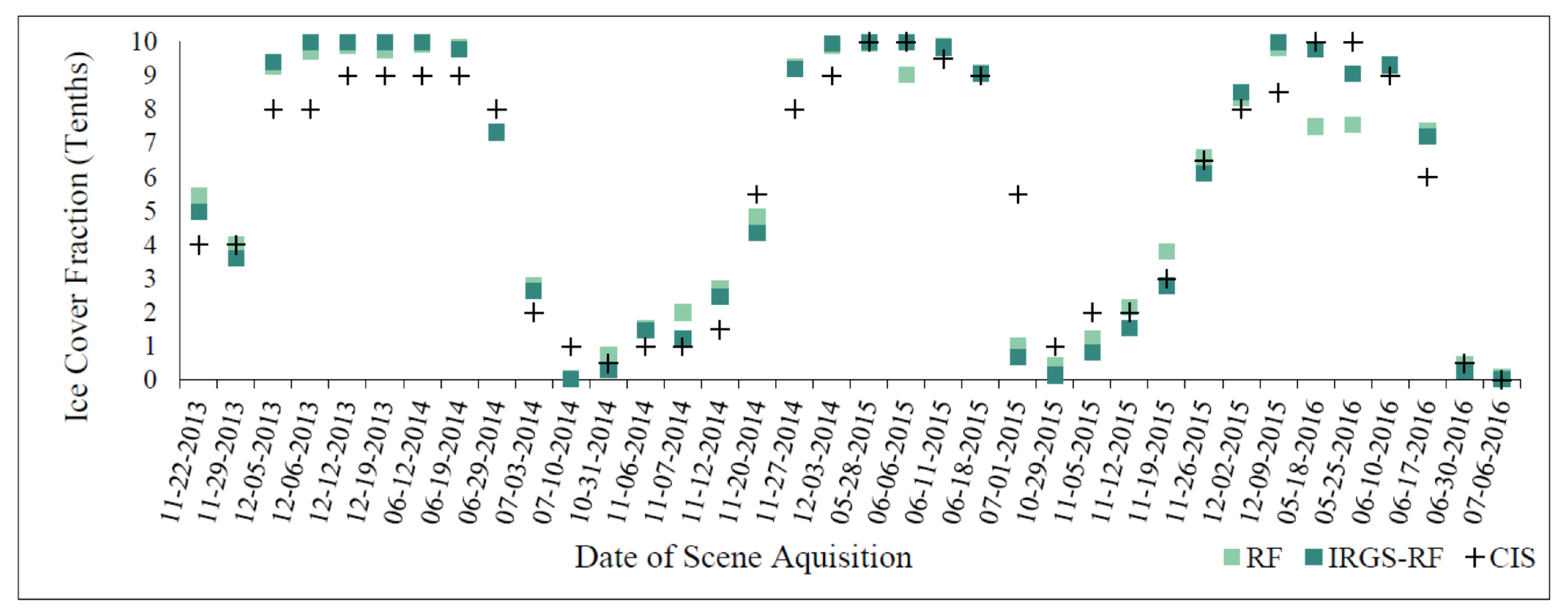
4. Results
5. Discussion
6. Conclusions
Author Contributions
Funding
Acknowledgments
Conflicts of Interest
Appendix A. Software and Hardware Specifications
Appendix A.1. Software
Appendix A.2. Hardware
- For IRGS-Manual classification: Intel i7 4790 with 16 GB RAM
- For RF, SVM, IRGS-RF and IRGS-SVM: Intel i7 6700K with 32 GB RAM
References
- Prowse, T.; Alfredsen, K.; Beltaos, S.; Bonsal, B.; Duguay, C.; Korhola, A.; McNamara, J.; Vincent, W.F.; Vuglinsky, V.; Weyhenmeyer, G.A. Arctic freshwater ice and its climatic role. Ambio 2011, 40, 46–52. [Google Scholar] [CrossRef][Green Version]
- Brown, L.; Duguay, C. The fate of lake ice in the North American Arctic. Cryosphere 2011, 5, 869. [Google Scholar] [CrossRef]
- Hewitt, B.; Lopez, L.; Gaibisels, K.; Murdoch, A.; Higgins, S.; Magnuson, J.; Paterson, A.; Rusak, J.; Yao, H.; Sharma, S. Historical trends, drivers, and future projections of ice phenology in small north temperate lakes in the Laurentian Great Lakes Region. Water 2018, 10, 70. [Google Scholar] [CrossRef]
- Magnuson, J.J.; Robertson, D.M.; Benson, B.J.; Wynne, R.H.; Livingstone, D.M.; Arai, T.; Assel, R.A.; Barry, R.G.; Card, V.; Kuusisto, E.; et al. Historical trends in lake and river ice cover in the Northern Hemisphere. Science 2000, 289, 1743–1746. [Google Scholar] [CrossRef] [PubMed]
- Sharma, S.; Blagrave, K.; Magnuson, J.J.; O’Reilly, C.M.; Oliver, S.; Batt, R.D.; Magee, M.R.; Straile, D.; Weyhenmeyer, G.A.; Winslow, L.; et al. Widespread loss of lake ice around the Northern Hemisphere in a warming world. Nat. Clim. Chang. 2019, 9, 227. [Google Scholar] [CrossRef]
- Brown, L.C.; Duguay, C.R. The response and role of ice cover in lake-climate interactions. Prog. Phys. Geogr. 2010, 34, 671–704. [Google Scholar] [CrossRef]
- Brown, R.D.; Duguay, C.R.; Goodison, B.E.; Prowse, T.D.; Ramsay, B.; Walker, A.E. Freshwater ice monitoring in Canada-an assessment of Canadian contributions for global climate monitoring. In Proceedings of the 16th IAHR International Symposium on Ice, Dunedin, New Zealand, 2–6 December 2002; Volume 1, pp. 368–376. [Google Scholar]
- Geldsetzer, T.; Van Der Sanden, J. Identification of polarimetric and nonpolarimetric C-band SAR parameters for application in the monitoring of lake ice freeze-up. Can. J. Remote Sens. 2013, 39, 263–275. [Google Scholar] [CrossRef]
- Howell, S.E.; Brown, L.C.; Kang, K.K.; Duguay, C.R. Variability in ice phenology on Great Bear Lake and Great Slave Lake, Northwest Territories, Canada, from SeaWinds/QuikSCAT: 2000–2006. Remote Sens. Environ. 2009, 113, 816–834. [Google Scholar] [CrossRef]
- Soh, L.K.; Tsatsoulis, C. Unsupervised segmentation of ERS and RADARSAT sea ice images using multiresolution peak detection and aggregated population equalization. Int. J. Remote Sens. 1999, 20, 3087–3109. [Google Scholar]
- Nghiem, S.V.; Leshkevich, G.A. Satellite SAR remote sensing of Great Lakes ice cover, Part 1. Ice backscatter signatures at C band. J. Great Lakes Res. 2007, 33, 722–735. [Google Scholar] [CrossRef]
- Kwok, R.; Cunningham, G.; Holt, B. An approach to identification of sea ice types from spaceborne SAR data. Microw. Remote Sens. Sea Ice 1992, 68, 355–360. [Google Scholar]
- Sobiech, J.; Dierking, W. Observing lake-and river-ice decay with SAR: Advantages and limitations of the unsupervised k-means classification approach. Ann. Glaciol. 2013, 54, 65–72. [Google Scholar] [CrossRef]
- Yu, Q.; Clausi, D.A. SAR sea-ice image analysis based on iterative region growing using semantics. IEEE Trans. Geosci. Remote Sens. 2007, 45, 3919–3931. [Google Scholar] [CrossRef]
- Yu, Q.; Clausi, D.A. IRGS: Image segmentation using edge penalties and region growing. IEEE Trans. Pattern Anal. Mach. Intell. 2008, 30, 2126–2139. [Google Scholar] [PubMed]
- Haarpaintner, J.; Solbø, S. Automatic ice-ocean discrimination in SAR imagery. Norut IT-Rep. 2007, 6, 28. [Google Scholar]
- Zakhvatkina, N.Y.; Alexandrov, V.Y.; Johannessen, O.M.; Sandven, S.; Frolov, I.Y. Classification of sea ice types in ENVISAT synthetic aperture radar images. IEEE Trans. Geosci. Remote Sens. 2012, 51, 2587–2600. [Google Scholar] [CrossRef]
- Leigh, S.; Wang, Z.; Clausi, D.A. Automated ice–water classification using dual polarization SAR satellite imagery. IEEE Trans. Geosci. Remote Sens. 2013, 52, 5529–5539. [Google Scholar] [CrossRef]
- Liu, H.; Guo, H.; Zhang, L. SVM-based sea ice classification using textural features and concentration from RADARSAT-2 dual-pol ScanSAR data. IEEE J. Sel. Top. Appl. Earth Obs. Remote Sens. 2014, 8, 1601–1613. [Google Scholar] [CrossRef]
- Zakhvatkina, N.; Korosov, A.; Muckenhuber, S.; Sandven, S.; Babiker, M. Operational algorithm for ice–water classification on dual-polarized RADARSAT-2 images. In High Resolution Sea Ice Monitoring Using Space Borne Synthetic Aperture Radar; Copernicus Publications: Göttingen, Germany, 2017. [Google Scholar]
- Han, H.; Hong, S.H.; Kim, H.c.; Chae, T.B.; Choi, H.J. A study of the feasibility of using KOMPSAT-5 SAR data to map sea ice in the Chukchi Sea in late summer. Remote Sens. Lett. 2017, 8, 468–477. [Google Scholar] [CrossRef]
- Shen, X.; Zhang, J.; Zhang, X.; Meng, J.; Ke, C. Sea ice classification using Cryosat-2 altimeter data by optimal classifier–feature assembly. IEEE Geosci. Remote Sens. Lett. 2017, 14, 1948–1952. [Google Scholar] [CrossRef]
- Soh, L.K.; Tsatsoulis, C.; Gineris, D.; Bertoia, C. ARKTOS: An intelligent system for SAR sea ice image classification. IEEE Trans. Geosci. Remote Sens. 2004, 42, 229–248. [Google Scholar] [CrossRef]
- Clausi, D.; Qin, A.; Chowdhury, M.; Yu, P.; Maillard, P. MAGIC: MAp-guided ice classification system. Can. J. Remote Sens. 2010, 36, S13–S25. [Google Scholar] [CrossRef]
- Kim, M.; Im, J.; Han, H.; Kim, J.; Lee, S.; Shin, M.; Kim, H.C. Landfast sea ice monitoring using multisensor fusion in the Antarctic. GIScience Remote Sens. 2015, 52, 239–256. [Google Scholar] [CrossRef]
- Zakhvatkina, N.; Smirnov, V.; Bychkova, I. Satellite sar data-based sea ice classification: An overview. Geosciences 2019, 9, 152. [Google Scholar] [CrossRef]
- Han, H.; Im, J.; Kim, M.; Sim, S.; Kim, J.; Kim, D.j.; Kang, S.H. Retrieval of melt ponds on arctic multiyear sea ice in summer from terrasar-x dual-polarization data using machine learning approaches: A case study in the chukchi sea with mid-incidence angle data. Remote Sens. 2016, 8, 57. [Google Scholar] [CrossRef]
- Geldsetzer, T.; Sanden, J.v.d.; Brisco, B. Monitoring lake ice during spring melt using RADARSAT-2 SAR. Can. J. Remote Sens. 2010, 36, S391–S400. [Google Scholar] [CrossRef]
- Liu, H.; Guo, H.; Li, X.M.; Zhang, L. An approach to discrimination of sea ice from open water using SAR data. In Proceedings of the International Geoscience and Remote Sensing Symposium (IGARSS), Beijing, China, 10–15 July 2016; pp. 4865–4867. [Google Scholar]
- Ochilov, S.; Clausi, D.A. Operational SAR sea-ice image classification. IEEE Trans. Geosci. Remote Sens. 2012, 50, 4397–4408. [Google Scholar] [CrossRef]
- Li, F.; Clausi, D.A.; Wang, L.; Xu, L. A semi-supervised approach for ice-water classification using dual-polarization SAR satellite imagery. In Proceedings of the IEEE Conference on Computer Vision and Pattern Recognition Workshops, Boston, MA, USA, 7–12 June 2015; pp. 28–35. [Google Scholar]
- Wang, J.; Duguay, C.; Clausi, D.; Pinard, V.; Howell, S. Semi-automated classification of lake ice cover using dual polarization RADARSAT-2 imagery. Remote Sens. 2018, 10, 1727. [Google Scholar] [CrossRef]
- MacDonald, D.; Associates Ltd. RADARSAT-2 Product Description. 2018. Available online: https://mdacorporation.com/docs/default-source/technical-documents/geospatial-services/52-1238_rs2_product_description.pdf?sfvrsn=10 (accessed on 23 April 2020).
- Vincent, L.; Soille, P. Watersheds in digital spaces: An efficient algorithm based on immersion simulations. IEEE Trans. Pattern Anal. Mach. Intell. 1991, 6, 583–598. [Google Scholar] [CrossRef]
- Yu, P.; Qin, A.; Clausi, D.A. Feature extraction of dual-pol SAR imagery for sea ice image segmentation. Can. J. Remote Sens. 2012, 38, 352–366. [Google Scholar] [CrossRef]
- Granitto, P.M.; Furlanello, C.; Biasioli, F.; Gasperi, F. Recursive feature elimination with random forest for PTR-MS analysis of agroindustrial products. Chemom. Intell. Lab. Syst. 2006, 83, 83–90. [Google Scholar] [CrossRef]
- Chavan, G.S.; Manjare, S.; Hegde, P.; Sankhe, A. A survey of various machine learning techniques for text classification. Int. J. Eng. Trends Technol. 2014, 15, 288–292. [Google Scholar] [CrossRef][Green Version]
- Shrivastava, R.; Mahalingam, H.; Dutta, N. Application and evaluation of random forest classifier technique for fault detection in bioreactor operation. Chem. Eng. Commun. 2017, 204, 591–598. [Google Scholar] [CrossRef]
- Duguay, C.R.; Pultz, T.J.; Lafleur, P.M.; Drai, D. RADARSAT backscatter characteristics of ice growing on shallow sub-Arctic lakes, Churchill, Manitoba, Canada. Hydrol. Process. 2002, 16, 1631–1644. [Google Scholar] [CrossRef]
- Clausi, D.A. MAGIC System. 2008. Available online: https://uwaterloo.ca/vision-image-processing-lab/research-demos/magic-system (accessed on 23 April 2020).
- Pedregosa, F.; Varoquaux, G.; Gramfort, A.; Michel, V.; Thirion, B.; Grisel, O.; Blondel, M.; Prettenhofer, P.; Weiss, R.; Dubourg, V.; et al. Scikit-learn: Machine Learning in Python. J. Mach. Learn. Res. 2011, 12, 2825–2830. [Google Scholar]


| Scene ID | SAR Acquisition Date (M/D/Y) | Acquisition Time UTC (hh:mm:ss) | Ascending (A)/ Descending (D) |
|---|---|---|---|
| 20131122_142937 | 11/22/2013 | 14:29:37 | D |
| 20131129_142532 | 11/29/2013 | 14:25:32 | D |
| 20131205_145035 | 12/05/2013 | 14:50:35 | D |
| 20131206_142120 | 12/06/2013 | 14:21:21 | D |
| 20131212_144618 | 12/12/2013 | 14:46:18 | D |
| 20131219_144152 | 12/19/2013 | 14:41:52 | D |
| 20140612_143755 | 06/12/2014 | 14:37:55 | D |
| 20140619_143342 | 06/19/2014 | 14:33:42 | D |
| 20140629_144205 | 06/19/2014 | 14:42:05 | D |
| 20140703_142514 | 07/03/2014 | 14:25:14 | D |
| 20140710_142114 | 07/10/2014 | 14:21:14 | D |
| 20141031_142522 | 10/31/2014 | 14:25:22 | D |
| 20141106_145027 | 11/06/2014 | 14:50:27 | D |
| 20141107_142115 | 11/07/2014 | 14:21:15 | D |
| 20141112_013553 | 11/12/2014 | 01:35:53 | A |
| 20141120_144206 | 11/20/2014 | 14:42:06 | D |
| 20141127_143745 | 11/27/2014 | 14:37:45 | D |
| 20141203_012332 | 12/03/2014 | 01:23:32 | A |
| 20150528_142923 | 05/28/2015 | 14:29:23 | D |
| 20150606_012716 | 06/06/2015 | 01:27:16 | A |
| 20150611_142104 | 06/11/2015 | 14:21:04 | D |
| 20150618_141641 | 06/18/2015 | 14:16:41 | D |
| 20150701_143743 | 07/01/2015 | 14:37:43 | D |
| 20151029_143745 | 10/29/2015 | 14:37:45 | D |
| 20151105_143336 | 11/05/2015 | 14:33:36 | D |
| 20151112_142917 | 11/12/2015 | 14:29:17 | D |
| 20151119_142512 | 11/19/2015 | 14:25:12 | D |
| 20151126_142102 | 11/26/2015 | 14:21:02 | D |
| 20151202_144602 | 12/02/2015 | 14:46:02 | D |
| 20151209_144152 | 12/09/2015 | 14:41:52 | D |
| 20160518_144544 | 05/18/2016 | 14:45:44 | D |
| 20160525_144140 | 05/25/2016 | 14:41:40 | D |
| 20160610_013545 | 06/10/2016 | 01:35:45 | A |
| 20160617_013133 | 06/17/2016 | 01:31:33 | A |
| 20160630_015219 | 06/30/2016 | 01:52:19 | A |
| 20160706_141626 | 07/06/2016 | 14:16:26 | D |
| Window Size (Pixels) | Step Size (Pixels) |
|---|---|
| 5 by 5 | 1 |
| 11 by 11 | 1 |
| 25 by 25 | 1 |
| 25 by 25 | 5 |
| 51 by 51 | 5 |
| 51 by 51 | 10 |
| 51 by 51 | 20 |
| 101 by 101 | 10 |
| 101 by 101 | 20 |
| Feature Rank | Polarization | Feature Name | Window Size | Step Size |
|---|---|---|---|---|
| 1 | HV | GLCM ASM | 25 by 25 | 1 |
| 2 | HV | GLCM COR | 25 by 25 | 1 |
| 3 | HV | GLCM ASM | 25 by 25 | 5 |
| 4 | HV | GLCM ENT | 11 by 11 | 1 |
| 5 | HV | GLCM ASM | 11 by 11 | 1 |
| 6 | HH | GLCM HOM | 101 by 101 | 10 |
| 7 | HH | GLCM ASM | 11 by 11 | 1 |
| 8 | HH | GLCM MU | 51 by 51 | 20 |
| 9 | HV | GLCM ASM | 51 by 51 | 5 |
| 10 | HH | GLCM COR | 25 by 25 | 1 |
| 11 | HH | GLCM ASM | 25 by 25 | 1 |
| 12 | HV | GLCM STD | 25 by 25 | 5 |
| 13 | HV | GLCM STD | 11 by 11 | 1 |
| 14 | HH | GLCM INV | 101 by 101 | 10 |
| 15 | HH | GLCM MU | 51 by 15 | 10 |
| 16 | HH | GLCM HOM | 51 by 51 | 5 |
| 17 | HH | GLCM MU | 51 by 51 | 5 |
| 18 | HV | GLCM ASM | 51 by 51 | 10 |
| 19 | HV | GLCM HOM | 25 by 25 | 5 |
| 20 | HH | GLCM ASM | 25 by 25 | 5 |
| 21 | HH | GLCM MU | 101 by 101 | 10 |
| 22 | HH | GLCM ASM | 5 by 5 | 1 |
| 23 | HH | GLCM HOM | 101 by 101 | 20 |
| 24 | HH | GLCM COR | 11 by 11 | 1 |
| 25 | HH | GLCM MU | 5 by 5 | 1 |
| 26 | HH | GLCM HOM | 25 by 25 | 1 |
| 27 | HH | Pixel Average | 25 by 25 | 1 |
| 28 | HV | GLCM ASM | 101 by 101 | 10 |
| 29 | HH | GLCM ASM | 51 by 51 | 5 |
| 30 | HV | GLCM INV | 25 by 25 | 5 |
| 31 | HH | Pixel Average | 5 by 5 | 1 |
| Scene ID | IRGS-Manual | SVM | RF | IRGS-SVM | IRGS-RF |
|---|---|---|---|---|---|
| 20131122_142937 | 81.9 | 68.3 | 87.8 | 83.5 | 88.8 |
| 20131129_142532 | 86.8 | 63.3 | 87.8 | 61.9 | 89.7 |
| 20131205_145035 | 98.8 | 85.8 | 97.8 | 98.5 | 98.0 |
| 20131206_142120 | 97.5 | 90.0 | 97.3 | 97.7 | 97.7 |
| 20131212_144618 | 100.0 | 91.8 | 97.3 | 99.3 | 100.0 |
| 20131219_144152 | 100.0 | 91.3 | 96.8 | 100.0 | 100.0 |
| 20140612_143755 | 99.5 | 90.5 | 98.8 | 99.5 | 99.5 |
| 20140619_143342 | 98.5 | 87.8 | 98.8 | 95.8 | 99.3 |
| 20140629_144205 | 92.3 | 68.8 | 85.8 | 64.3 | 85.0 |
| 20140703_142514 | 93.3 | 76.5 | 90.5 | 90.0 | 92.8 |
| 20140710_142114 | 99.2 | 78.0 | 99.2 | 87.4 | 99.7 |
| 20141031_142522 | 98.3 | 61.5 | 93.8 | 89.0 | 97.5 |
| 20141106_145027 | 92.0 | 33.5 | 95.8 | 27.3 | 95.0 |
| 20141107_142115 | 86.1 | 55.8 | 91.5 | 61.5 | 90.0 |
| 20141112_013553 | 88.5 | 54.0 | 93.8 | 54.3 | 93.8 |
| 20141120_144206 | 84.8 | 83.8 | 94.50 | 85.5 | 92.5 |
| 20141127_143745 | 86.0 | 81.0 | 94.3 | 84.8 | 98.5 |
| 20141203_012332 | 93.0 | 92.8 | 98.4 | 99.7 | 99.5 |
| 20150528_142923 | 98.8 | 88.6 | 99.5 | 100.0 | 100.0 |
| 20150606_012716 | 99.7 | 81.8 | 90.0 | 84.4 | 99.5 |
| 20150611_142104 | 98.5 | 97.5 | 99.3 | 97.8 | 99.5 |
| 20150618_141641 | 99.5 | 94.5 | 98.3 | 93.5 | 98.8 |
| 20150701_143743 | 87.5 | 10.3 | 89.0 | 3.8 | 92.8 |
| 20151029_143745 | 96.5 | 58.0 | 94.5 | 60.8 | 97.5 |
| 20151105_143336 | 96.0 | 74.0 | 92.5 | 80.1 | 95.2 |
| 20151112_142917 | 88.3 | 73.3 | 90.3 | 92.0 | 91.0 |
| 20151119_142512 | 88.3 | 75.8 | 87.3 | 90.5 | 93.8 |
| 20151126_142102 | 77.3 | 77.3 | 93.3 | 91.6 | 91.0 |
| 20151202_144602 | 84.0 | 82.8 | 98.0 | 96.3 | 98.8 |
| 20151209_144152 | 100.0 | 89.5 | 98.0 | 100.0 | 100.0 |
| 20160518_144544 | 100.0 | 84.3 | 72.3 | 99.0 | 95.5 |
| 20160525_144140 | 100.0 | 76.5 | 70.0 | 78.3 | 88.3 |
| 20160610_013545 | 97.5 | 87.8 | 99.0 | 91.2 | 98.5 |
| 20160617_013133 | 95.0 | 79.3 | 94.5 | 75.0 | 94.8 |
| 20160630_015219 | 93.3 | 28.0 | 96.8 | 27.5 | 99.0 |
| 20160706_141626 | 98.8 | 77.0 | 97.8 | 76.8 | 99.0 |
| Overall Accuracy | 93.8 | 74.7 | 93.3 | 81.1 | 95.8 |
| Ice Error | 2.6 | 6.3 | 3.3 | 2.3 | 1.9 |
| Open Water Error | 3.7 | 19.0 | 3.5 | 16.7 | 2.2 |
© 2020 by the authors. Licensee MDPI, Basel, Switzerland. This article is an open access article distributed under the terms and conditions of the Creative Commons Attribution (CC BY) license (http://creativecommons.org/licenses/by/4.0/).
Share and Cite
Hoekstra, M.; Jiang, M.; Clausi, D.A.; Duguay, C. Lake Ice-Water Classification of RADARSAT-2 Images by Integrating IRGS Segmentation with Pixel-Based Random Forest Labeling. Remote Sens. 2020, 12, 1425. https://doi.org/10.3390/rs12091425
Hoekstra M, Jiang M, Clausi DA, Duguay C. Lake Ice-Water Classification of RADARSAT-2 Images by Integrating IRGS Segmentation with Pixel-Based Random Forest Labeling. Remote Sensing. 2020; 12(9):1425. https://doi.org/10.3390/rs12091425
Chicago/Turabian StyleHoekstra, Marie, Mingzhe Jiang, David A. Clausi, and Claude Duguay. 2020. "Lake Ice-Water Classification of RADARSAT-2 Images by Integrating IRGS Segmentation with Pixel-Based Random Forest Labeling" Remote Sensing 12, no. 9: 1425. https://doi.org/10.3390/rs12091425
APA StyleHoekstra, M., Jiang, M., Clausi, D. A., & Duguay, C. (2020). Lake Ice-Water Classification of RADARSAT-2 Images by Integrating IRGS Segmentation with Pixel-Based Random Forest Labeling. Remote Sensing, 12(9), 1425. https://doi.org/10.3390/rs12091425