Neural Network Reflectance Prediction Model for Both Open Ocean and Coastal Waters

Abstract
1. Introduction
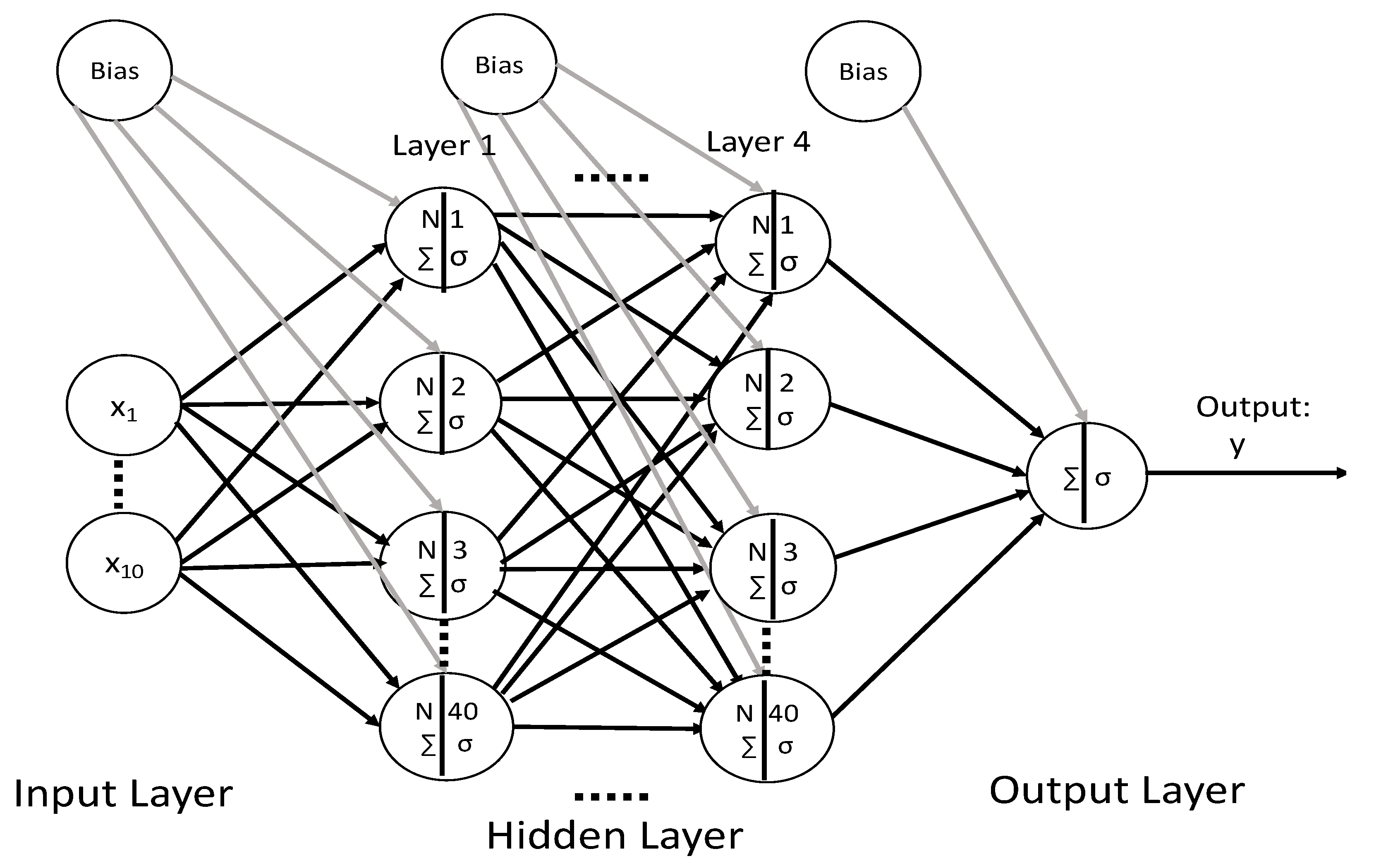
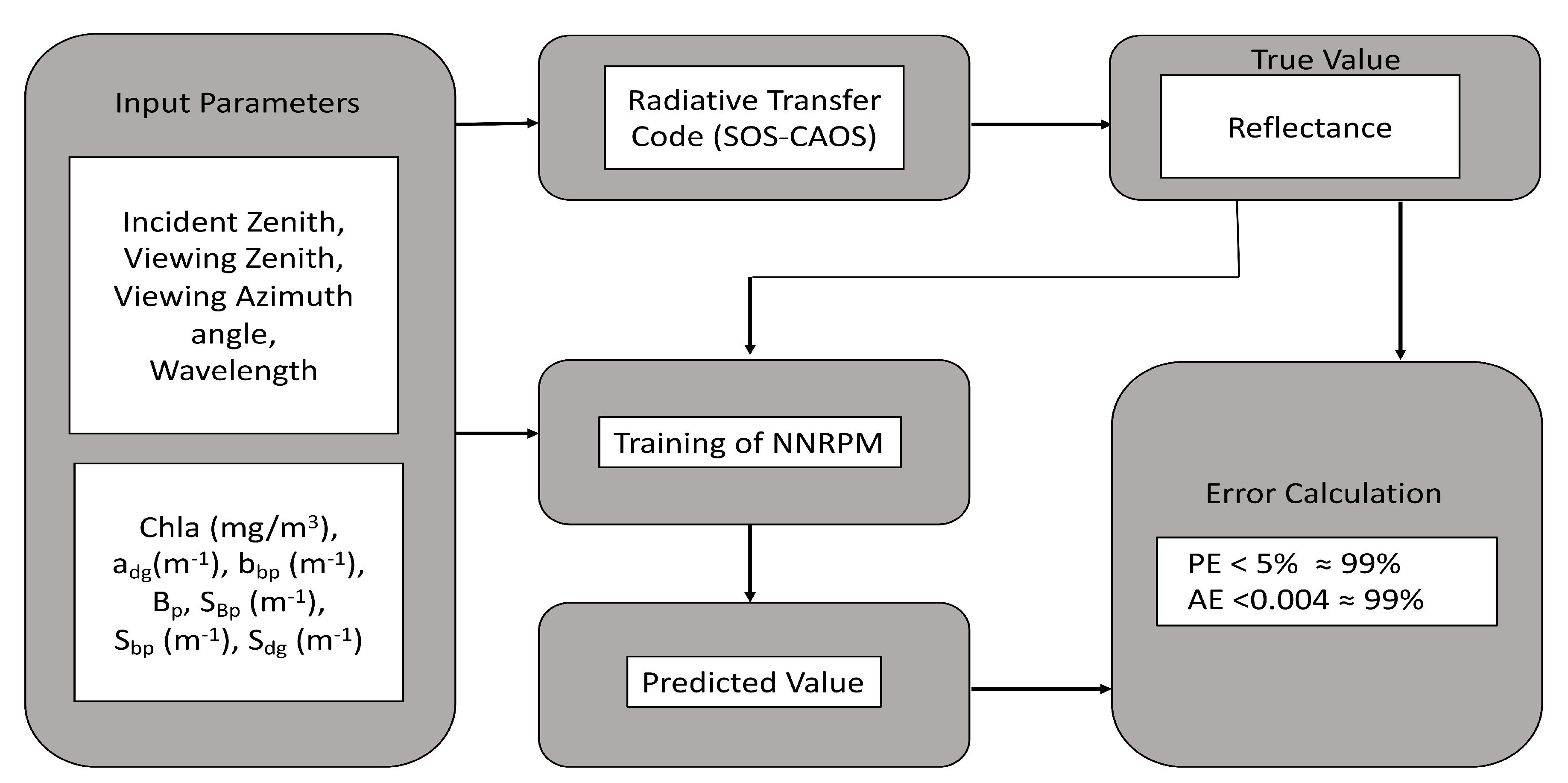
2. Methods
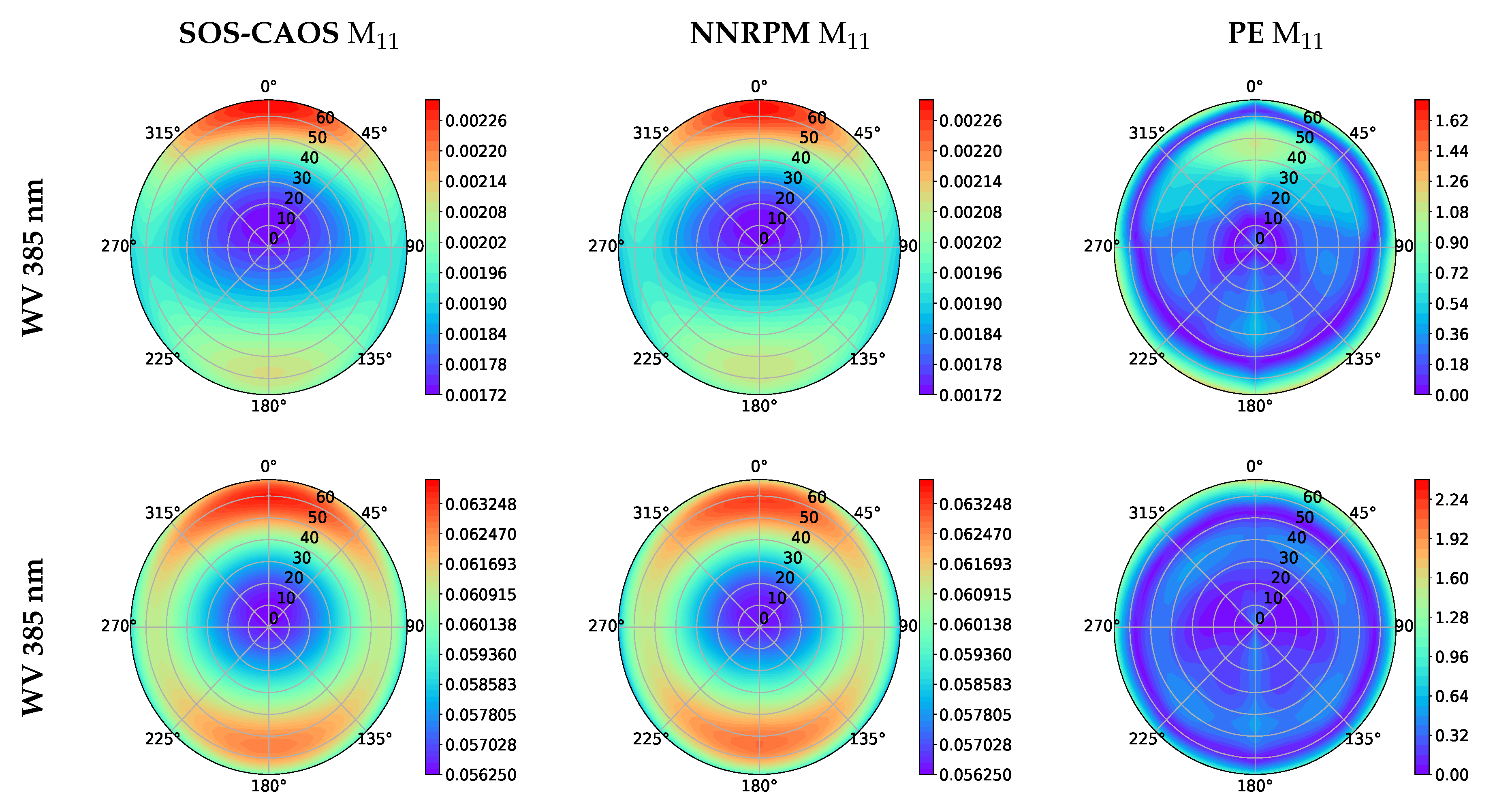
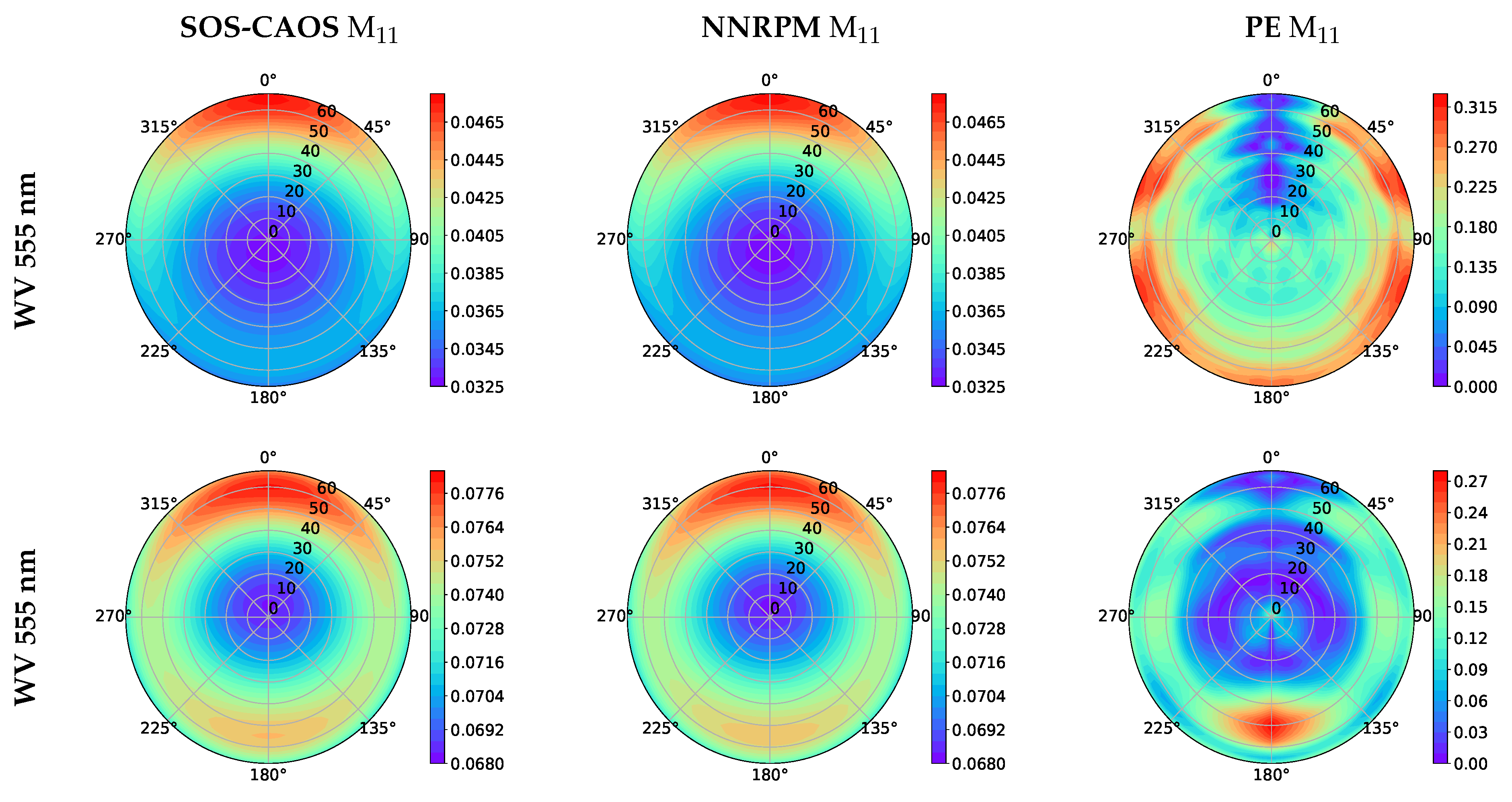
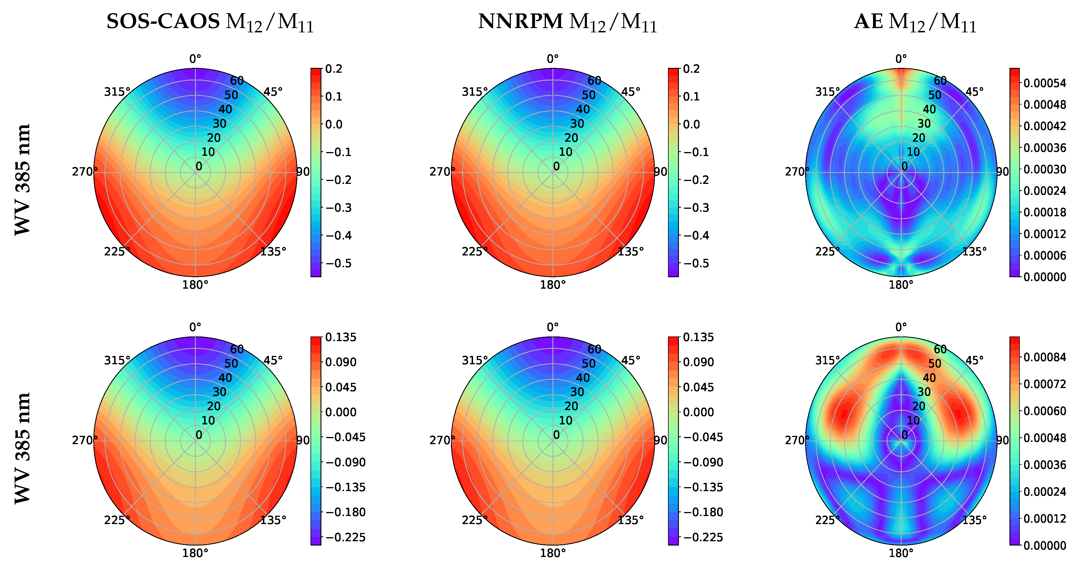
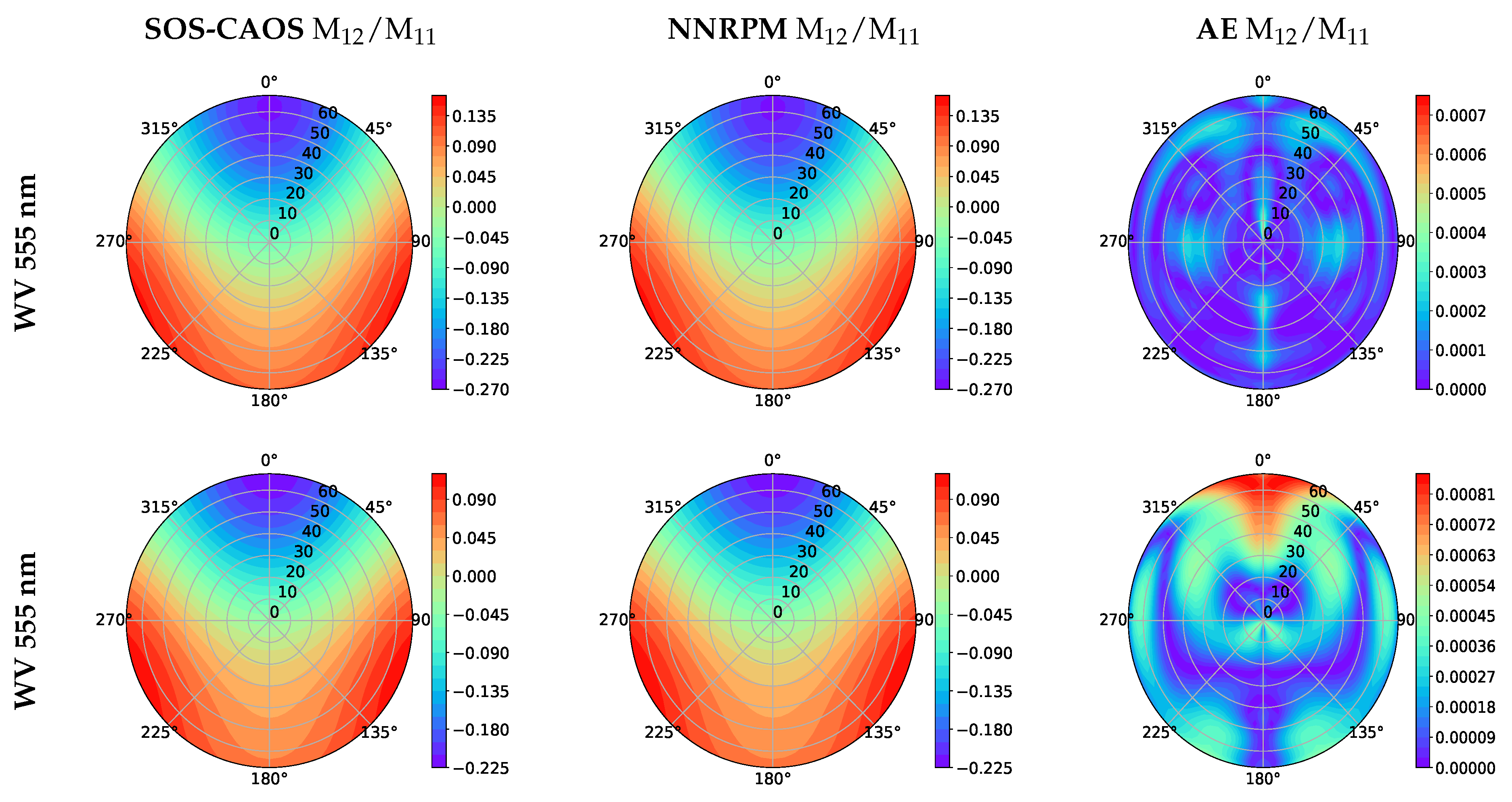
3. Results
- Order of scattering: 40
- Gaussian quadrature for ocean: 80
- Optical depth of the system (for wavelength 555 nm): 6986.19
- Scattering coefficient of phytoplankton and NAP particles, bp: 34.468 m−1
- System specifications: 2.8 GHz Intel Core i7 and memory of 16 GB 1600 MHz DDR3
4. Discussion
5. Conclusions
Author Contributions
Funding
Acknowledgments
Conflicts of Interest
References
- Antoine, D.; Morel, A. A multiple scattering algorithm for atmospheric correction of remotely sensed ocean colour (MERIS instrument): Principle and implementation for atmospheres carrying various aerosols including absorbing ones. Int. J. Remote Sens. 1999, 20, 1875–1916. [Google Scholar] [CrossRef]
- Fukushima, H.; Higurashi, A.; Mitomi, Y.; Nakajima, T.; Noguchi, T.; Tanaka, T.; Toratani, M. Correction of atmospheric effect on ADEOS/OCTS ocean color data: Algorithm description and evaluation of its performance. J. Oceanogr. 1998, 54, 417–430. [Google Scholar] [CrossRef]
- Gordon, H.R.; Wang, M. Retrieval of water-leaving radiance and aerosol optical thickness over the oceans with SeaWiFS: A preliminary algorithm. Appl. Opt. 1994, 33, 443–452. [Google Scholar] [CrossRef] [PubMed]
- Dierssen, H.M. Perspectives on empirical approaches for ocean color remote sensing of chlorophyll in a changing climate. Proc. Natl. Acad. Sci. USA 2010, 107, 17073–17078. [Google Scholar] [CrossRef] [PubMed]
- Hu, C.; Lee, Z.; Franz, B. Chlorophyll aalgorithms for oligotrophic oceans: A novel approach based on three band reflectance difference. J. Geophys. Res. Oceans 2012, 117, 1–25. [Google Scholar] [CrossRef]
- Shanmugam, P.; Ahn, Y.H.; Ryu, J.H.; Sundarabalan, B. An evaluation of inversion models for retrieval of inherent optical properties from ocean color in coastal and open sea waters around Korea. J. Oceanogr. 2010, 66, 815–830. [Google Scholar] [CrossRef]
- Boss, E.; Roesler, C. Over constrained linear matrix inversion with statistical selection. In Remote Sensing of Inherent Optical Properties: Fundamentals, Tests of Algorithms, and Applications; Volume 5 of Reports of the International Ocean Colour Coordinating Group; Lee, Z.P., Ed.; IOCCG: Dartmouth, NS, Canada, 2006; pp. 57–62. [Google Scholar]
- Garver, S.A.; Siegel, D.A. Inherent optical property inversion of ocean color spectra and its biogeochemical interpretation: 1. Time series from the Sargasso Sea. J. Geophys. Res. Oceans 1997, 102, 18607–18625. [Google Scholar] [CrossRef]
- Maritorena, S.; Siegel, D.A.; Peterson, A.R. Optimization of a semianalytical ocean color model for global-scale applications. Appl. Opt. 2002, 41, 2705–2714. [Google Scholar] [CrossRef]
- Gordon, H.R.; Brown, O.B.; Evans, R.H.; Brown, J.W.; Smith, R.C.; Baker, K.S.; Clark, D.K. A semianalytic radiance model of ocean color. J. Geophys. Res. Atmos. 1988, 93, 10909–10924. [Google Scholar] [CrossRef]
- IOCCG. Remote Sensing of Inherent Optical Properties: Fundamentals, Tests of Algorithms, and Applications. In Reports of the International Ocean Colour Coordinating Group; Lee, Z.P., Ed.; IOCCG: Dartmouth, NS, Canada, 2006; Volume 5. [Google Scholar]
- Ligi, M.; Kutser, T.; Kallio, K.; Attila, J.; Koponen, S.; Paavel, B.; Soomets, T.; Reinart, A. Testing the performance of empirical remote sensing algorithms in the Baltic Sea waters with modelled and in situ reflectance data. Oceanologia 2017, 59, 57–68. [Google Scholar] [CrossRef]
- Morel, A.; Gentili, B. A simple band ratio technique to quantify the colored dissolved and detrital organic material from ocean color remotely sensed data. Remote Sens. Environ. 2009, 113, 998–1011. [Google Scholar] [CrossRef]
- Franz, B.A.; Werdell, P.J. A generalized framework for modeling of inherent optical properties in ocean remote sensing applications. Proc. Ocean Opt. Anchorage Alaska 2010, 27, 1–3. [Google Scholar]
- Werdell, P.J.; McKinna, L.I.; Boss, E.; Ackleson, S.G.; Craig, S.E.; Gregg, W.W.; Lee, Z.; Maritorena, S.; Roesler, C.S.; Rousseaux, C.S.; et al. An overview of approaches and challenges for retrieving marine inherent optical properties from ocean color remote sensing. Prog. Oceanogr. 2018, 160, 186–212. [Google Scholar] [CrossRef] [PubMed]
- IOCCG. Remote Sensing of Ocean Colour in Coastal, and Other Optically-Complex, Waters. In Reports of the International Ocean Colour Coordinating Group; Sathyendranath, S., Ed.; IOCCG: Dartmouth, NS, Canada, 2000; Volume 3. [Google Scholar]
- IOCCG. Atmospheric Correction for Remotely-Sensed Ocean-Colour Products. In Reports of the International Ocean Colour Coordinating Group; Wang, M., Ed.; IOCCG: Dartmouth, NS, Canada, 2010; Volume 10. [Google Scholar]
- Deschamps, P.Y.; Bréon, F.M.; Leroy, M.; Podaire, A.; Bricaud, A.; Buriez, J.C.; Seze, G. The POLDER mission: Instrument characteristics and scientific objectives. IEEE Trans. Geosci. Remote Sens. 1994, 32, 598–615. [Google Scholar] [CrossRef]
- Cairns, B.; Russell, E.E.; Travis, L.D. Research scanning polarimeter: Calibration and ground-based measurements. In Polarization: Measurement, Analysis, and Remote Sensing II. Int. Soc. Opt. Photonics 1999, 3754, 186–196. [Google Scholar]
- Diner, D.J.; Xu, F.; Garay, M.J.; Martonchik, J.V.; Rheingans, B.E.; Geier, S.; Davis, A.; Hancock, B.R.; Jovanovic, V.M.; Bull, M.A.; et al. the Airborne Multiangle SpectroPolarimetric Imager (AirMSPI): A new tool for aerosol and cloud remote sensing. Atmos. Meas. Tech. 2013, 6, 2007–2025. [Google Scholar] [CrossRef]
- Snik, F.; Rietjens, J.H.; Van Harten, G.; Stam, D.M.; Keller, C.U.; Smit, J.M.; Laan, E.C.; Verlaan, A.L.; Ter Horst, R.; Navarro, R.; et al. SPEX: The spectropolarimeter for planetary exploration. Space Telescopes and Instrumentation 2010: Optical, Infrared, and Millimeter Wave. Int. Soc. Opt. Photonics 2010, 7731. [Google Scholar] [CrossRef]
- Martins, J.V.; Fernandez-Borda, R.; McBride, B.; Remer, L.; Barbosa, H.M. The Harp Hype Ran Gular Imaging Polarimeter and the Need for Small Satellite Payloads with High Science Payoff for Earth Science Remote Sensing. In Proceedings of the IGARSS 2018— IEEE International Geoscience and Remote Sensing Symposium, Valencia, Spain, 22–27 July 2018; pp. 6304–6307. [Google Scholar]
- Werdell, P.J.; Behrenfeld, M.J.; Bontempi, P.S.; Boss, E.; Cairns, B.; Davis, G.T.; Franz, B.A.; Gliese, U.B.; Gorman, E.T.; Hasekamp, O.; et al. the Plankton, Aerosol, Cloud, ocean Ecosystem mission: Status, science, advances. Bull. Am. Meteorol. Soc. 2019, 100, 1775–1794. [Google Scholar] [CrossRef]
- Chowdhary, J.; Cairns, B.; Mishchenko, M.I.; Hobbs, P.V.; Cota, G.F.; Redemann, J.; Rutledge, K.; Holben, B.N.; Russell, E. Retrieval of aerosol scattering and absorption properties from photopolarimetric observations over the ocean during the CLAMS experiment. J. Atmos. Sci. 2005, 62, 1093–1117. [Google Scholar] [CrossRef]
- Hasekamp, O.P.; Litvinov, P.; Butz, A. Aerosol properties over the ocean from PARASOL multiangle photopolarimetric measurements. J. Geophys. Res. Atmos. 2011, 116, 2156–2202. [Google Scholar] [CrossRef]
- Xu, F.; Dubovik, O.; Zhai, P.W.; Diner, D.J.; Kalashnikova, O.V.; Seidel, F.C.; Litvinov, P.; Bovchaliuk, A.; Garay, M.J.; van Harten, G.; et al. Joint retrieval of aerosol and water-leaving radiance from multispectral, multiangular and polarimetric measurements over ocean. Atmos. Meas. Tech. 2016, 9, 2877–2907. [Google Scholar] [CrossRef]
- Gao, M.; Zhai, P.W.; Franz, B.; Hu, Y.; Knobelspiesse, K.; Werdell, P.J.; Ibrahim, A.; Cairns, B.; Chase, A. Inversion of multi-angular polarimetric measurements over open and coastal ocean waters: A joint retrieval algorithm for aerosol and water leaving radiance properties. Atmos. Meas. Tech. 2019, 12, 3921–3941. [Google Scholar] [CrossRef]
- Fan, C.; Fu, G.; Di Noia, A.; Smit, M.; Rietjens, H.H.J.; Ferrare, A.R.; Burton, S.; Li, Z.; Hasekamp, P.O. Use of a Neural Network-Based Ocean Body Radiative Transfer Model for Aerosol Retrievals from Multi-Angle Polarimetric Measurements. Remote Sens. 2019, 11, 2877. [Google Scholar] [CrossRef]
- Gao, M.; Zhai, P.W.; Franz, B.; Hu, Y.; Knobelspiesse, K.; Werdell, P.J.; Ibrahim, A.; Xu, F.; Cairns, B. Retrieval of aerosol properties and water-leaving reflectance from multi-angular polarimetric measurements over coastal waters. Opt. Express 2018, 26, 8968–8989. [Google Scholar] [CrossRef] [PubMed]
- Kou, L.; Labrie, D.; Chylek, P. Refractive indices of water and ice in the 0.65-to 2.5-μm spectral range. Appl. Opt. 1993, 32, 3531–3540. [Google Scholar] [CrossRef] [PubMed]
- Pope, R.M.; Fry, E.S. Absorption spectrum (380–700 nm) of pure water. II. Integrating cavity measurements. Appl. Opt. 1997, 36, 8710–8723. [Google Scholar] [CrossRef]
- Zhang, X.; Hu, L. Scattering by pure seawater at high salinity. Opt. Express 2009, 17, 12685–12691. [Google Scholar] [CrossRef]
- Morel, A. Optical properties of pure water and pure sea water. Opt. Asp. Oceanogr. 1974, 1, 1–24. [Google Scholar]
- Bricaud, A.; Morel, A.; Babin, M.; Allali, K.; Claustre, H. Variations of light absorption by suspended particles with chlorophyll a concentration in oceanic (case 1) waters: Analysis and implications for bio-optical models. J. Geophys. Res. Oceans 1998, 103, 31033–31044. [Google Scholar] [CrossRef]
- Werdell, P.J.; Franz, B.A.; Bailey, S.W.; Feldman, G.C.; Claustre, H. Generalized ocean color inversion model for retrieving marine inherent optical properties. Appl. Opt. 2013, 52, 2019–2037. [Google Scholar] [CrossRef]
- Werdell, P.J.; McKinna, L.I.W. Sensitivity of Inherent Optical Properties From Ocean Reflectance Inversion Models to Satellite Instrument Wavelength Suites. Front. Earth Sci. 2019, 7, 54. [Google Scholar] [CrossRef] [PubMed]
- Fournier, G.R.; Forand, J.L. Analytic phase function for ocean water. In Ocean Optics XII; International Society for Optics and Photonics: Bergen, Norway, 1994; pp. 194–201. [Google Scholar]
- Sullivan, J.M.; Twardowski, M.S. Angular shape of the oceanic particulate volume scattering function in the backward direction. Appl. Opt. 2009, 48, 6811–6819. [Google Scholar] [CrossRef] [PubMed]
- Mobley, C.D.; Sundman, L.K. Phase function effects on oceanic light fields. Appl. Opt. 2002, 41, 1035–1050. [Google Scholar] [CrossRef] [PubMed]
- Voss, K.J.; Fry, E.S. Measurement of the Mueller matrix for ocean water. Appl. Opt. 1984, 23, 4427–4439. [Google Scholar] [CrossRef]
- Kokhanovsky, A.A. Parameterization of the Mueller matrix of oceanic waters. J. Geophys. Res. Oceans 2003, 108, 3175. [Google Scholar] [CrossRef]
- Zhai, P.W.; Knobelspiesse, K.; Ibrahim, A.; Franz, B.A. Water-leaving contribution to polarized radiation field over ocean. Opt. Express 2017, 25, A689–A708. [Google Scholar] [CrossRef]
- Zhai, P.W.; Hu, Y.; Trepte, C.R.; Lucker, P.L. A vector radiative transfer model for coupled atmosphere and ocean systems based on successive order of scattering method. Opt. Express 2009, 17, 2057–2079. [Google Scholar] [CrossRef]
- Zhai, P.W.; Yongxiang, H.; Chowdhary, J.; Trepte, C.R.; Lucker, P.L.; Josset, D.B. A vector radiative transfer model for coupled atmosphere and ocean systems with a rough interface. J. Quant. Spectrosc. Radiat. Transf. 2010, 111, 1025–1040. [Google Scholar] [CrossRef]
- Lawless, R.; Xie, Y.; Yang, P.; Kattawar, G.W.; Laszlo, I. Polarization and effective Mueller matrix for multiple scattering of light by nonspherical ice crystals. Opt. Express 2006, 14, 6381–6393. [Google Scholar] [CrossRef]
- Kattawar, G.W.; Adams, C.N. Stokes vector calculations of the submarine light field in an atmosphere-ocean with scattering according to a Rayleigh phase matrix: Effect of interface refractive index on radiance and polarization. Limnol. Oceanogr. 1989, 34, 1453–1472. [Google Scholar] [CrossRef]
- MathWorks. Deep Learning Toolbox; The MathWorks Inc.: Natick, MA, USA, 2019. [Google Scholar]
- Smith, J.A. LAI inversion using a back-propagation neural network trained with a multiple scattering model. IEEE Trans. Geosci. Remote Sens. 1993, 31, 1102–1106. [Google Scholar] [CrossRef]
- Smith, J.A. Multilayer feedforward networks are universal approximators. Neural Netw. 1989, 2, 359–366. [Google Scholar]
- Abuelgasim, A.A.; Gopal, S.; Strahler, A.H. Forward and inverse modelling of canopy directional reflectance using a neural network. Int. J. Remote Sens. 1998, 19, 453–471. [Google Scholar] [CrossRef]
- Gron, A. Hands-On Machine Learning with Scikit-Learn and TensorFlow: Concepts, Tools, and Techniques to Build Intelligent Systems, 1st ed.; O’Reilly Media, Inc.: Newton, MA, USA, 2017. [Google Scholar]
- Marquardt, D.W. An algorithm for least-squares estimation of nonlinear parameters. J. Soc. Ind. Appl. Math. 1963, 11, 431–441. [Google Scholar] [CrossRef]
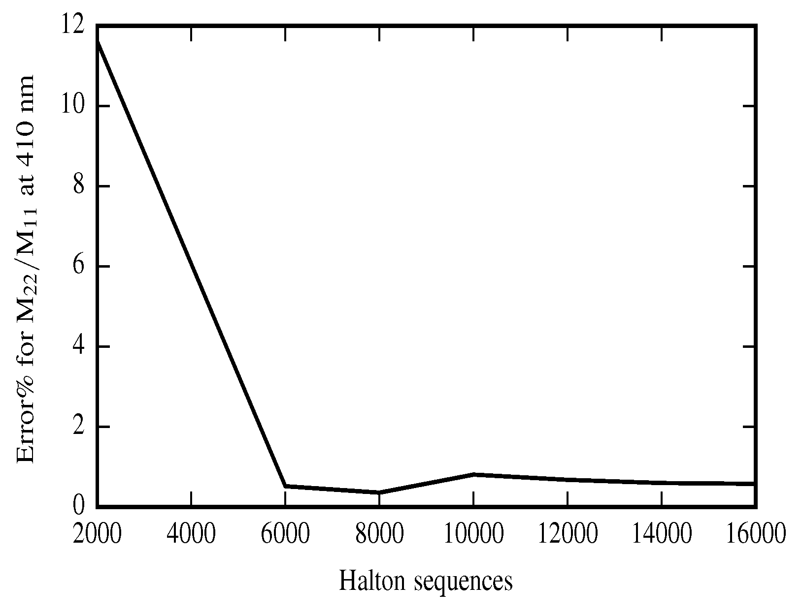
- Loyola, R.; Diego, G.; Pedergnana, M.; Gimeno, S.G. Smart sampling and incremental function learning for very large high dimensional data. Neural Netw. 2016, 78, 75–87. [Google Scholar] [CrossRef]
- Halton, J.H. On the efficiency of certain quasi-random sequences of points in evaluating multi-dimensional integrals. Numer. Math. 1960, 2, 84–90. [Google Scholar] [CrossRef]
- Pernot, P.; Savin, A. Probabilistic performance estimators for computational chemistry methods: The empirical cumulative distribution function of absolute errors. J. Chem. Phys. 2018, 148, 241707. [Google Scholar] [CrossRef]
- James, G.; Witten, D.; Hastie, T.; Tibshirani, R. An Introduction to Statistical Learning: With Applications in R; Springer Publishing Company: Berlin, Germany, 2014. [Google Scholar]
- Gallant, A.R.; White, H. There exists a neural network that does not make avoidable mistakes. In Proceedings of the International Conference on Neural Networks, San Diego, CA, USA, 24–27 July 1988. [Google Scholar]
- Nicodemus, F.E.; Richmond, J.C.; Hsia, J.J.; Ginsberg, I.W.; Limperis, T. Geometrical Considerations and Nomenclature for Reflectance; NBS Monograph; National Bureau of Standards: Washington, DC, USA, 1992. [Google Scholar]


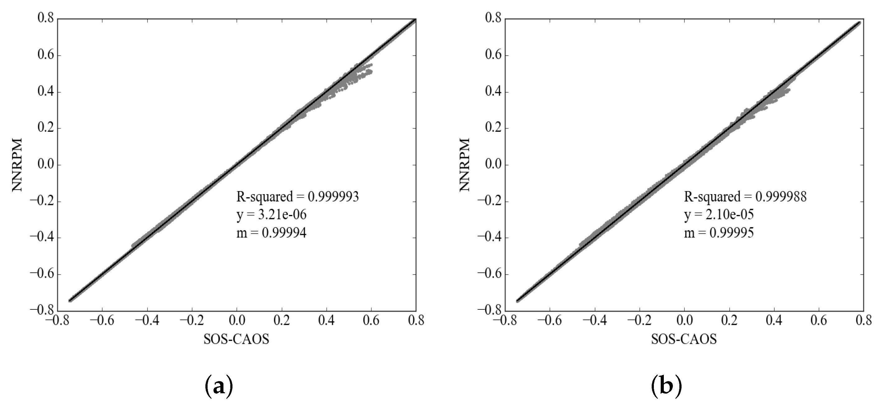
| Parameter | Chla | adg(440) | bbp(660) | Bp(660) | Sdg | Sbp | SBp |
|---|---|---|---|---|---|---|---|
| Unit | mg/m3 | m−1 | m−1 | nm−1 | nm−1 | nm−1 | |
| Min | ∼0.0 | ∼0.0 | ∼0.0 | ∼0.0 | 0.01 | 0.0 | −0.2 |
| Max | 30.0 | 2.5 | 0.1 | 0.05 | 0.02 | 0.5 | 0.2 |
| M11 | M21/M11 | M31/M11 | DoLP | |
|---|---|---|---|---|
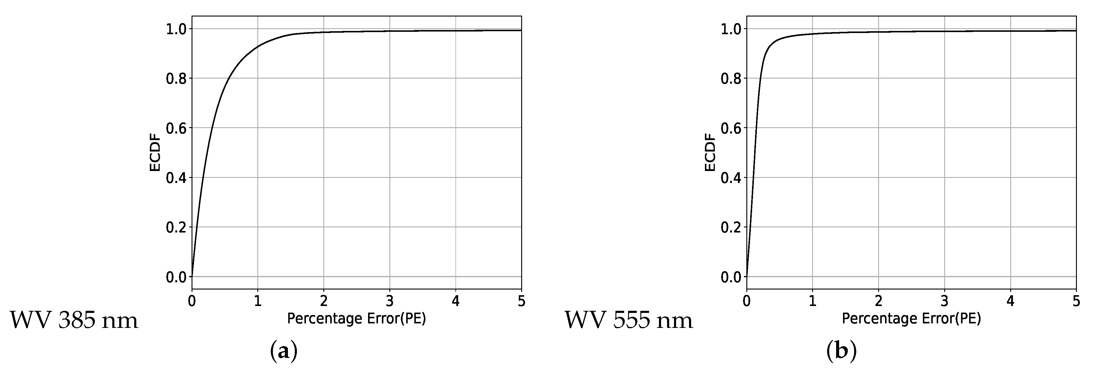
| Wavelength (nm) | PE < 5% | AE < 0.004 | AE < 0.004 | AE < 0.002 |
| 385 | 99.64 | 99.78 | 99.83 | 99.23 |
| 410 | 99.25 | 99.68 | 99.82 | 98.90 |
| 440 | 99.39 | 99.75 | 99.73 | 98.97 |
| 470 | 99.24 | 99.77 | 99.70 | 98.98 |
| 555 | 99.29 | 99.78 | 99.71 | 98.79 |
| 670 | 99.29 | 99.75 | 99.80 | 99.02 |
| 863.5 | 99.57 | 99.93 | 99.92 | 99.71 |
| 870 | 99.55 | 99.94 | 99.92 | 99.72 |
| M12/M11 | M22/M11 | M32/M11 | |
|---|---|---|---|
| Wavelength (nm) | AE < 0.004 | AE < 0.004 | AE < 0.004 |
| 385 | 99.67 | 99.43 | 99.56 |
| 410 | 99.38 | 99.64 | 99.40 |
| 440 | 99.50 | 99.30 | 99.37 |
| 470 | 99.26 | 99.13 | 99.08 |
| 555 | 98.68 | 99.54 | 99.24 |
| 670 | 99.53 | 99.70 | 99.667 |
| 863.5 | 99.97 | 99.68 | 99.79 |
| 870 | 99.92 | 99.71 | 99.72 |
| M13/M11 | M23/M11 | M33/M11 | |
|---|---|---|---|
| Wavelength (nm) | AE < 0.004 | AE < 0.004 | AE < 0.004 |
| 385 | 98.89 | 99.34 | 99.42 |
| 410 | 98.83 | 99.23 | 99.39 |
| 440 | 98.78 | 99.05 | 99.29 |
| 470 | 98.00 | 98.86 | 99.17 |
| 555 | 98.20 | 98.31 | 99.32 |
| 670 | 98.56 | 99.52 | 99.63 |
| 863.5 | 99.95 | 99.73 | 99.74 |
| 870 | 99.92 | 99.69 | 99.74 |
© 2020 by the authors. Licensee MDPI, Basel, Switzerland. This article is an open access article distributed under the terms and conditions of the Creative Commons Attribution (CC BY) license (http://creativecommons.org/licenses/by/4.0/).
Share and Cite
Mukherjee, L.; Zhai, P.-W.; Gao, M.; Hu, Y.; A. Franz, B.; Werdell, P.J. Neural Network Reflectance Prediction Model for Both Open Ocean and Coastal Waters. Remote Sens. 2020, 12, 1421. https://doi.org/10.3390/rs12091421
Mukherjee L, Zhai P-W, Gao M, Hu Y, A. Franz B, Werdell PJ. Neural Network Reflectance Prediction Model for Both Open Ocean and Coastal Waters. Remote Sensing. 2020; 12(9):1421. https://doi.org/10.3390/rs12091421
Chicago/Turabian StyleMukherjee, Lipi, Peng-Wang Zhai, Meng Gao, Yongxiang Hu, Bryan A. Franz, and P. Jeremy Werdell. 2020. "Neural Network Reflectance Prediction Model for Both Open Ocean and Coastal Waters" Remote Sensing 12, no. 9: 1421. https://doi.org/10.3390/rs12091421
APA StyleMukherjee, L., Zhai, P.-W., Gao, M., Hu, Y., A. Franz, B., & Werdell, P. J. (2020). Neural Network Reflectance Prediction Model for Both Open Ocean and Coastal Waters. Remote Sensing, 12(9), 1421. https://doi.org/10.3390/rs12091421