Remote Sensing Retrieval of Total Phosphorus in the Pearl River Channels Based on the GF-1 Remote Sensing Data

Abstract

Total phosphorus (TP) concentration is one of the indicators for surface water quality evaluation. In this study, an indirect algorithm was proposed to retrieve TP concentration. This algorithm retrieves the TP concentration in urban waters based on Gaofen-1 (GF-1) remote sensing data. The algorithm uses the correlation between remote-sensing reflectance, optically significant constituents of water (chlorophyll, suspended sediment, and organic matter (excluding algae)), and TP to establish a retrieval model. First, the concentrations of optically active components are retrieved using a semi-analytical model. Second, the correlation between TP and optically active components is used to retrieve the TP concentration in waters. The GF-1 remote sensing data for 7 August 2015 were used to perform remote sensing retrieval of TP concentration in the Pearl River channels in Guangzhou, China. The results show that the TP concentration in most areas of the Front Channel, Western Channel, Guangzhou Channel, and the western part of the Back Channel was higher than 0.2 mg/L, while the TP concentration in the middle and eastern parts of the Back Channel was generally lower than 0.2 mg/L. The mean absolute percentage error of the retrieval is 24.18%. The experimental results show that the model is suitable for remote sensing retrieval of TP in urban waters in Guangzhou.

1. Introduction

Recently, pollution in coastal waters and inland waters has become increasingly severe. Nitrogen and phosphorus nutrients that enter waters through various channels are important reasons for eutrophication [1,2,3,4]. Conventional water quality sampling and monitoring methods are time-consuming and demand large efforts and costs. Only local water quality information about the monitored section can be obtained. Water quality status and changes in a large area cannot be accurately obtained. Remote sensing technology has the advantages of a broad monitoring range, fast speed, and low costs, which facilitate long-term continuous monitoring. Remote sensing technology can also be used to detect problems such as pollution sources and a pollutant diffusion status, which are hardly possible by using conventional monitoring methods. As a result, remote sensing technology is increasingly employed in water quality monitoring studies [5,6].

Nutrients are not optically active substances. They have weak absorption and scattering energy of light in natural waters. Current remote sensing retrieval studies primarily retrieve nutrients using direct and indirect methods based on empirical models [7]. In general, models are only applicable to waters in a specific study area. Direct methods can be applied to obtain the relationship between nutrients and spectral data by using techniques such as regression analysis and the differential spectrum technique. For example, Huang et al. (2015) employed two bands of the Geostationary Ocean Color Imager (GOCI) remote sensing data to construct a total phosphorus (TP) retrieval model, and discovered that the TP concentration has a certain correlation with chlorophyll and suspended sediment (SS) (R² > 0.52). Moses et al. (2014) established a regression equation between the TP concentration and the reflectance of the red band. The retrieval results showed that the predicted values were well correlated with the measured values (R² = 0.76). Li et al. (2017) used the reflectance of four bands of Landsat 8 OLI to construct an empirical retrieval model for total nitrogen and TP, respectively. Gao et al. (2015) used corresponding combinations of reflectance of four bands of HJ-1A CCD2 images to retrieve the TP in Chaohu Lake. Indirect methods generally establish retrieval models for nutrients based on the relationship between nutrients and chlorophyll, SS, water temperature, etc. For instance, Goes et al. (1999) established a regression model of sea surface temperature and chlorophyll-a (Chla) to retrieve the nitrate concentration of surface waters in the North Pacific. Ana et al. (2008) proposed using the difference between the estimated temperature of upwelling and the sea surface temperature to improve the method of Goes et al. Li et al. (2017) employed the monthly mean rainfall, wind speed, temperature, and cumulative sunshine duration to estimate the monthly mean total nitrogen concentration and TP concentration in the Xin’anjiang Reservoir. Baustian et al. (2018) estimated the TP retention in coastal wetlands around the Laurentian Great Lakes in North America.

Currently, studies of remote sensing retrieval of TP primarily focus on coastal waters or large lakes and large reservoirs [4,6,7,8,9,10,11,12,13]. Relatively few studies address remote sensing retrieval of TP in rivers. Most retrieval models are directly established based on the relationship between TP and water reflectance or the relationship between TP and SS and chlorophyll. Previous studies have indicated that the TP concentration in waters has a strong correlation with optically active substances, such as SS and chlorophyll [6,8,13]. However, for rivers that flow through cities in Guangdong Province, China, organic pollution in urban river channels is usually severe. Therefore, when the indirect method is used to retrieve the TP concentration in urban river channels, the effects of SS, chlorophyll, and organic pollutants should be comprehensively considered.

The purpose of this study is to construct an indirect algorithm suitable for TP concentration retrieval in urban rivers. First, based on the measured water leaving reflectance and water quality analysis results, a semi-analytical algorithm was used to retrieve the concentration of suspended sediment (SS), chlorophyll (Chl, in this study, represented by the chlorophyll-a, Chla), and organic matter (excluding algae, organic pollutants in water mainly refer to the complex organic materials dominated by oxygen-consuming organic matter in water, including dissolved organics and suspended organic particles, which are similar to the organic pollution characterized by Chemical Oxygen Demand (COD). Therefore, the permanganate index (COD_Mn) is used to characterize them in this study in urban river channels. Regression equations between TP concentration and other water quality parameters were then constructed, according to the laboratory test results of water quality. Second, a retrieval model of TP concentration was established. Last, Gaofen-1 (GF-1) remote sensing images were used to retrieve the TP in the Pearl River channels in Guangzhou, and the performance of the retrieval algorithm was evaluated.

2. Materials and Methods

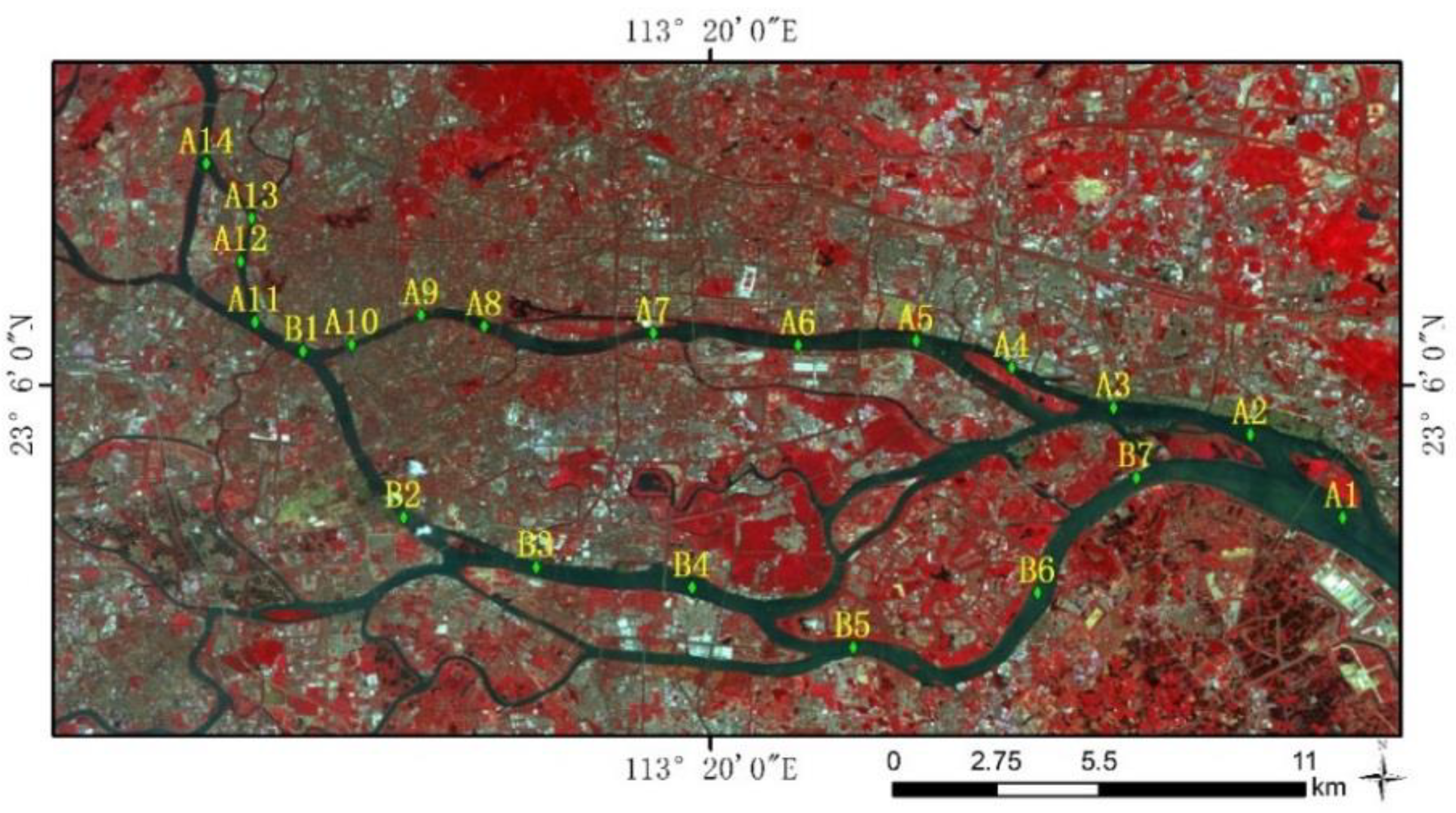
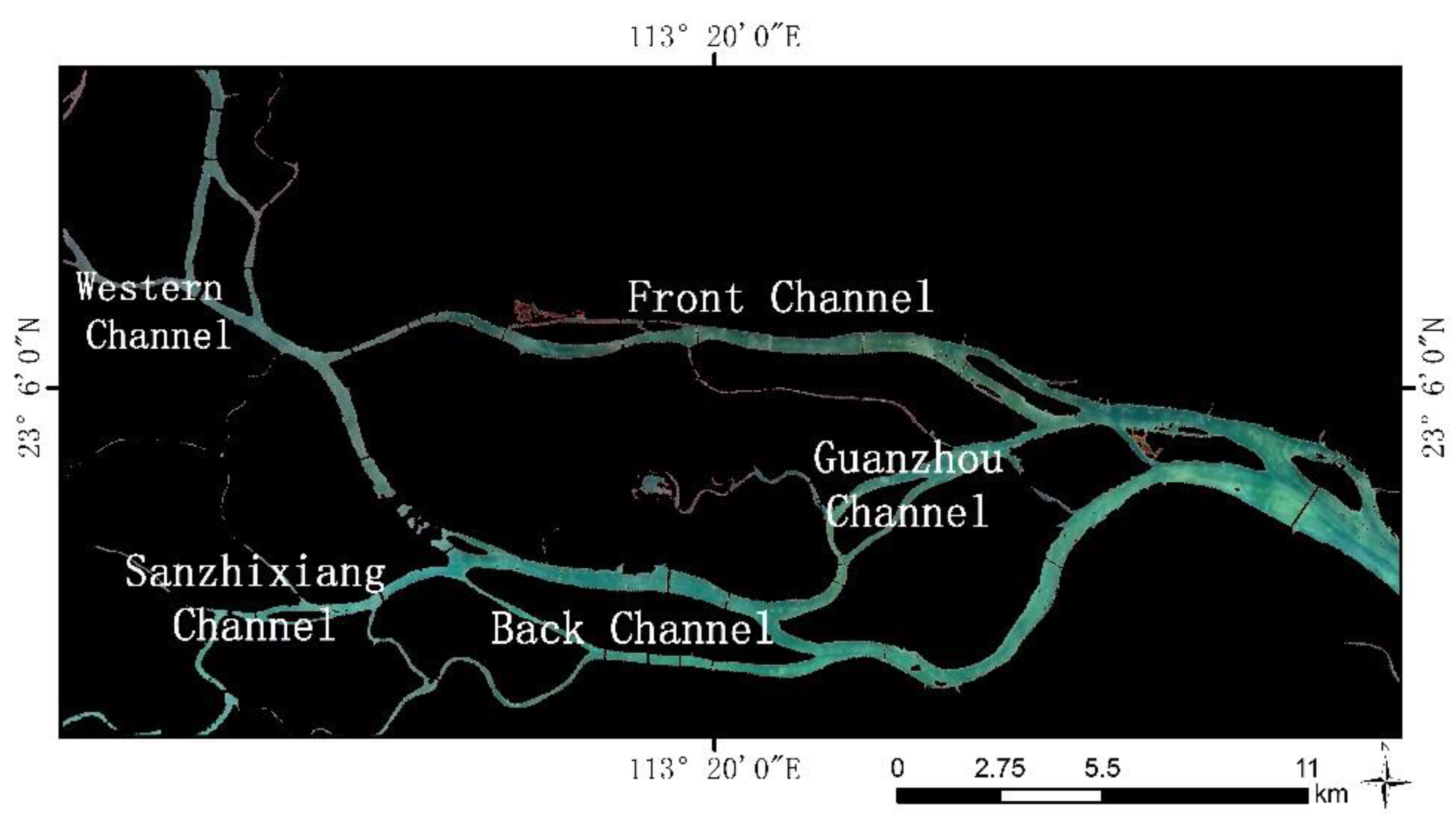
2.1. Study Area

The Pearl River channels in Guangzhou, Guangdong Province, China is selected as the study area, as shown in Figure 1. In Guangzhou City near the Pearl River, the urban population is large, and industry and commerce are well developed. As a result, water pollution is severe in the Pearl River channels, which comprise a typical example of urban river channels.

2.2. Data

2.2.1. Measured Water Leaving Reflectance Data

In the two days prior to the GF-1 satellite imaging (5-6 August 2015), simultaneous water spectral measurement, water quality sampling, and an analysis experiment were performed. In the week prior to the satellite imaging, the weather conditions in Guangzhou were satisfactory with a gentle breeze and no precipitation. The sampling sites of the experiment are shown in Figure 2. The water leaving reflectance curves were measured with a spectrometer (ASD FieldSpec3 spectrometer manufactured by the U.S. Company ASD) with an effective measurement spectral range of 350–2500 nm. Note that A1–A14 denotes the sampling sites on 5 August 2015, and B1–B7 denotes the sampling sites on 6 August 2015. At each sampling site, the measurement of the water spectrum by the Above-Water Method [14] was repeated multiple times when performing the water spectrum measurement to eliminate random errors.

2.2.2. GF-1 Remote Sensing Data

The remote sensing data used in this study is a multispectral remote sensing image of China’s GF-1 satellite, with a spatial resolution of 16 m and an imaging date of 7 August 2015. The GF-1 satellite was launched by the China Aerospace Science and Technology Corporation (CASC) in April 2013. The wide field of view (WFV) imaging system is one of the key instruments operating onboard the GF-1 satellite, which includes four integrated cameras with a 16-m spatial resolution [15]. The satellite parameters of GF-1 are shown in

Table 1. The satellite parameters of GF-1.

Orbit Parameters		16-m Multispectral Data Parameters
Items	Parameters	Bands	Spectral Range (μm)	Swath Width (km)	Temporal Resolution
Orbit type	Sun Synchronous orbit	Band1	0.45–0.52	800 (four cameras combined)	2 (day)
Orbit height	645 km	Band2	0.52–0.59
Orbit inclination	98.0506°	Band3	0.63–0.69
Descending node	10:30 AM at local time	Band4	0.77–0.89
Return period	41 (day)

[16].

The steps to obtain GF-1 remote sensing data of the Pearl River channels in Guangzhou are shown in Figure 3. First, the remote sensing data were preprocessed. By using Equation (1) [17], radiometric calibration of the GF-1 multispectral remote sensing data was performed to convert the satellite-based observation values into radiance.

$$L_e\left({\lambda }_e\right)=Gain·DN+Offset$$

(1)

where ${\mathit{L}}_{\mathit{e}}\left({\mathit{\lambda }}_{\mathit{e}}\right)$ is the converted radiance, DN is the satellite-based observation value, gain is the calibration slope, and offset is the offset of the absolute calibration coefficient. An image-based automatic inversion algorithm of aerosol optical density proposed by Qin et al. (2015) is employed for atmospheric correction to obtain multispectral reflectance data [18]. Second, water extraction is performed. The Multilayer Perceptron (MLP) neural network model is used to extract the water bodies in Guangzhou from the reflectance data in the study area obtained after data preprocessing [19]. The water extraction results are shown in Figure 4.

2.2.3. Water Quality Analysis Data

During the experiment of the Guangzhou section of the Pearl River on 5–6 August 2015, water samples were collected at each sampling site of the experiment after the measurement of the water leaving reflectance spectrum of the water. Five liters of the surface water was collected at each sampling point and stored in a plastic sampling bottle, which was sent to the laboratory within 24 hours for water quality detection and analysis. The detection methods of water quality parameters are shown in

Table 2. The detection methods of water quality parameters.

Items	Measurement Units	Detection Limits	Detection Methods
CODMn	mg/L	0.5	Volumetric method, Water quality--Determination of permanganate index (GB/T 11892-1989) [This standard refers to the international standard ISO 8467:1986 (revised to ISO 8467:1993): Water quality--Determination of permanganate index]
Chla	μg/L	0.025	Photometry method, water and waste water monitoring and analysis method, 4th Edition (compiled by State Environmental Protection Administration, published by China Environmental Science Press, 2002), Chapter I, Section V (I), Part V
SS	mg/L	4	Gravimetric method
TP	mg/L	0.01	Ammonium molybdate spectrophotometric method, Water quality--Determination of total phosphorus--Ammonium molybdate spectrophotometric method (GB/T 11893-1989)

. (Note: The water quality test was performed by the China National Analytical Center, Guangzhou).

2.2.4. Optical Parameters of Water Components

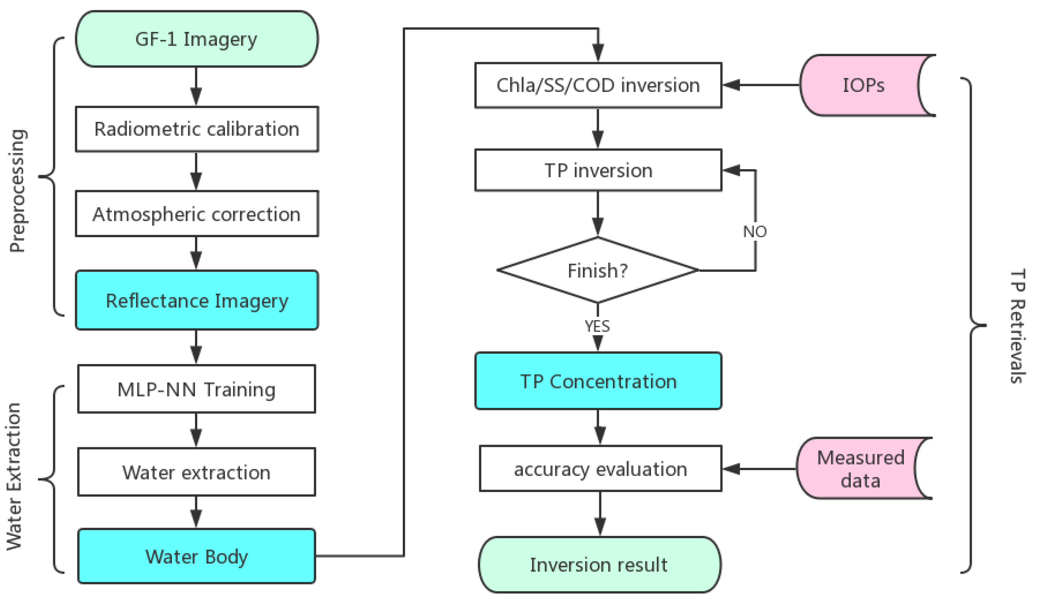
To establish semi-analytical models for retrieving concentrations of Chl, SS, and organic matter components, the inherent optical properties (IOPs) of each component are required. In the study of ocean color remote sensing, the optically active components in water are usually divided into suspended particles, photosynthetic pigments, and colored dissolved organic matter (CDOM or Gelbstoff, yellow substances) [20,21,22,23]. The IOPs of pure water, SS, Chl, CDOM, and other components can be obtained from relevant research literature [24,25,26,27,28,29,30,31,32,33,34]. However, for the urban reach of the Pearl River channels in Guangzhou, the organic pollution is usually serious and the composition of organic pollutants is complex. Li et al. (2002) used Gas Chromatography-Mass Spectrometry (GC-MS) to determine the Haiyin section water of the Pearl River channel in Guangzhou [35]. The results show that there were many kinds of organic pollutants in the water with a large concentration. Sixty organic compounds were separated and identified, including alkanes, alcohols, ketones, aromatics, polycyclic aromatic hydrocarbons, phenols, acids, and amines, which were from different pollution sources. Zheng et al. (2016) analyzed the water samples of the Back Channel of the Pearl River in Guangzhou and found that the dissolved organic matter (DOM) was more enriched in carbohydrate, amide, carboxylic, and aliphatic compounds [36]. CDOM (historically referred to as Gelbstoff, humic matter, or yellow substances due to its high humic matter content [33,37,38]) is a part of DOM. For the water body of the Back Channel of the Pearl River channel in Guangzhou, analysis results of Shong et al. (2013) show that only about 10% of DOM is humic matter (CDOM) [39]. The composition of organic pollutants in urban river channels in Guangzhou is complex and cannot be simply characterized by the optical parameters of CDOM. Therefore, it is necessary to measure the absorption coefficient and scattering coefficient of organic matter in urban water bodies with complex organic pollutants such as the water body of the Pearl River in Guangzhou. Brando et al. (2009) proposed a semi-analytical inversion method to estimate the concentration of optically active components (chlorophyll, CDOM, and non-algal particles (NAP)) in water. In this study, considering the serious organic pollution in the water body of the Pearl River in Guangzhou and the low content of CDOM in the dissolved organic matter, a semi-analytical inversion method for estimating the concentration of chlorophyll, organic matter, and non-algal particles (in this study, represented by the suspended sediment, SS) in the water is constructed based on the improved Brando algorithm. In the algorithm, the optical parameters of Chl are obtained from the results of Brando [27,28], and the optical parameters of pure water and SS are obtained from the results of Deng [30] and He [31]. The optical parameters of Chl, pure water, and SS are shown in Figure 5. The absorption coefficient and scattering coefficient of organic matter were measured using the measurement method proposed by He et al. (2011). Water samples from heavily polluted waters in the urban area of Guangzhou were collected, and then the optical parameters of organic matter were measured.

2.3. Methods

2.3.1. TP Regression Analysis

Currently, the retrieval of TP in waters is primarily carried out by establishing a relationship between TP and remote-sensing reflectance or other water quality parameters (such as Chla and SS) [4,6,7,8,9,12]. In this study, regression analysis of TP concentration in the Pearl River channel in Guangzhou with the water sample quality analysis results and the measured spectral data shows that TP in the Pearl River channels in Guangzhou is well correlated with other water quality parameters. The correlation coefficient between TP concentration and a combination of COD_Mn, Chl, and SS is the highest (R² = 0.9056, F value for F-test = 47.886). Therefore, the regression in Equation (2) is selected for TP retrieval.

$$C_{TP}=coe{f}_c*C_c+coe{f}_s*C_s+coe{f}_0*C_0+coe{f}_{\mathsf{\epsilon }}$$

(2)

where $C_{TP}$, $C_c$, $C_s,$ and $C_0$ represent the concentration of TP, Chl, SS, and COD_Mn, respectively, in water. $coe{f}_c$, $coe{f}_s$, $coe{f}_0$, and $coe{f}_{\mathsf{\epsilon }}$ are the retrieval coefficients.

2.3.2. Semi-Analytical Model for Water Quality Retrieval

To retrieve TP concentration using Equation (2), the concentration of optically active components, such as Chl, SS, and DOM (organic pollutant composition, represented by the permanganate index, COD_Mn), must be obtained by the corresponding water quality retrieval models. Water quality retrieval models include empirical models, semi-analytical models, and analytical models [40]. Empirical models directly establish the relationship between water quality and remote sensing spectra, which cannot be directly used for water bodies with different water quality conditions. Analytical models are based on clear physical concepts. However, obtaining many parameters is difficult. Semi-analytical models are based on radiative transfer theory and appropriately simplified for solution. Semi-analytical models are highly adaptable and have been extensively investigated. In general, water reflectance can be expressed as a function of optical parameters, observation geometry, and bottom reflectance of the relevant components of water bodies [20].

$$R_{rs}\left(\lambda \right)=f\left[\alpha \left(\lambda \right),\beta \left(\lambda \right),\rho \left(\lambda \right),H,{\theta }_w,\theta ,\mathsf{\phi }\right]$$

(3)

where $R_{rs}\left(\lambda \right)$ is the water-leaving reflectance, $\alpha \left(\lambda \right)$ is the absorption coefficient, $\beta \left(\lambda \right)$is the volume scattering function, $\rho \left(\lambda \right)$ is the bottom albedo, H is the bottom depth, and ${\theta }_w$ is subsurface solar zenith angle. $\theta$ is the subsurface viewing angle from nadir, and $\mathsf{\phi }$ is the viewing azimuth angle from the solar plane [20], respectively. Gordon constructed a semi-analytical model of water quality retrieval based on the IOPs of water quality components when studying ocean water color remote sensing [21,22,23,41].

$$R_{rs}\left(\lambda \right)=f\frac{b_b\left(\lambda \right)}{\alpha \left(\lambda \right)+b_b\left(\lambda \right)}=f\frac{b_b\left(\lambda \right)}{k\left(\lambda \right)}$$

(4)

where $f=0.0949+0.0794\frac{b_b\left(\lambda \right)}{\alpha \left(\lambda \right)+b_b\left(\lambda \right)}$ [21,22,41,42], $\alpha \left(\lambda \right)$ and $b_b\left(\lambda \right)$ are the total absorption coefficient and the total backscattering coefficient, $k$ is the extinction coefficient, $k\left(\lambda \right)=\alpha \left(\lambda \right)+b_b\left(\lambda \right)$, respectively, and $\lambda$ is the frequency of the corresponding spectral bands [27,42,43,44].

$$\alpha \left(\lambda \right)=a_w\left(\lambda \right)+{\displaystyle \sum }_{j=1}^n{a}_j\left(\lambda \right)*C_j$$

(5)

$$b_b\left(\lambda \right)=b_{bw}\left(\lambda \right)+{\displaystyle \sum }_{j=1}^n{b}_{bj}\left(\lambda \right)*C_j$$

(6)

where $a_w\left(\lambda \right)$ and $b_{bw}\left(\lambda \right)$ represent the absorption coefficient and backscattering coefficient of pure water, respectively, and $a_j\left(\lambda \right)$, $b_{bj}\left(\lambda \right)$, and $C_j$ represent the absorption coefficient, scattering coefficient, and concentration of the $j^{th}$ water quality component at unit concentration. Substituting Equations (5) and (6) into Equation (4) and disregarding the scattering effect of organic matter [21,28], the expression of the optical water-leaving reflectance $R_{rs}$ can be obtained.

$$R_{rs}(\lambda )=f\frac{b_{bw}\left(\lambda \right)+C_c{b}_{bc}\left(\lambda \right)+C_s{b}_{bs}\left(\lambda \right)}{{\alpha }_w\left(\lambda \right)+C_c{\alpha }_c\left(\lambda \right)+C_s{\alpha }_s\left(\lambda \right)+C_o{\alpha }_o\left(\lambda \right)+b_{bw}\left(\lambda \right)+C_c{b}_{bc}\left(\lambda \right)+C_s{b}_{bs}\left(\lambda \right)}$$

(7)

where $C_{comp}$ is the concentration of the water components, The subscript $comp$ can be $W$, $C$, $S,$ and $O$ represent pure water, Chla, SS, and COD_Mn, respectively.

2.3.3. TP Retrieval Model

After the optical parameters of each water component are obtained, the remote sensing retrieval model of optical water-leaving reflectance can be solved. From Equation (7), in order to express conciseness, the frequency $\lambda$ in Equation (7) and the subscript rs of the water leaving reflectance $R_{rs}$ are omitted, and the following equation can be established.

$$\begin{array}{c}\left[R_i{k}_{c_i}-f_i{b}_{b{c}_i}\right]C_C+\left[R_i{k}_{S_i}-f_i{b}_{b{S}_i}\right]C_S+R_i{\alpha }_{o_i}{C}_O=f_i{b}_{b{w}_i}-R_i{k}_{w_i}\end{array}$$

(8)

where $R$ is the water leaving reflectance at the corresponding band, $k$ is the extinction coefficient, $k_{comp}={\alpha }_{comp}+b_{comp}$. The subscript $comp$ can be $W$, $C$, $S$, and $O$, which represent pure water, Chl, SS, and organic matter (represented by the permanganate index, COD_Mn), respectively. The subscript $i$ corresponds to remote sensing data at the $i^{th}$ band. For the GF-1 multispectral remote sensing data, four multispectral bands exist. Selecting three of the four bands (in this study, band2-band4, i.e., green, red, and near-infrared bands are selected) and, substituting relevant parameters into Equation (8), a set of equations for the concentration of three water quality components is established, namely, Chl, SS, and COD_Mn. The concentration of each water quality component in the water can be solved.

$$\{\begin{array}{l}\left[R_1{k}_{c_1}-f_1{b}_{b{c}_1}\right]C_C+\left[R_1{k}_{S_1}-f_1{b}_{b{S}_1}\right]C_S+R_1{\alpha }_{o_1}{C}_O=f_1{b}_{b{w}_1}-R_1{k}_{w_1}\hfill \\ \left[R_2{k}_{c_2}-f_2{b}_{b{c}_2}\right]C_C+\left[R_2{k}_{S_2}-f_2{b}_{b{S}_2}\right]C_S+R_2{\alpha }_{o_2}{C}_O=f_2{b}_{b{w}_2}-R_2{k}_{w_2}\\ \left[R_3{k}_{c_3}-f_3{b}_{b{c}_3}\right]C_C+\left[R_3{k}_{S_3}-f_3{b}_{b{S}_3}\right]C_S+R_3{\alpha }_{o_3}{C}_O=f_3{b}_{b{w}_3}-R_3{k}_{w_3}\end{array}$$

(9)

Equation (9) can be rewritten as a linear matrix inversion method proposed by Hoge & Lyon [42,45,46,47]. The Hoogenboom et al. (1998) study, which used the linear matrix inversion method for inland water study on the Dutch Lake Braassem, is referred to as the Matrix Inversion Method (MIM) [46,47]:

$$\left[\begin{array}{c}{R}_1{k}_{c_1}-f_1{b}_{b{c}_1} R_1{k}_{S_1}-f_1{b}_{b{S}_1} R_1{\alpha }_{o_1}\\ R_2{k}_{c_2}-f_2{b}_{b{c}_2} R_2{k}_{S_2}-f_2{b}_{b{S}_2} R_2{\alpha }_{o_2}\\ R_3{k}_{c_3}-f_3{b}_{b{c}_3} R_3{k}_{S_3}-f_3{b}_{b{S}_3} R_3{\alpha }_{o_3}\end{array}\right]\left[\begin{array}{c}{C}_{\mathrm{c}}\\ C_{\mathrm{s}}\\ C_{\mathrm{o}}\end{array}\right]=\left[\begin{array}{c}{f}_1{b}_{b{w}_1}-R_1{k}_{w_1}\\ f_2{b}_{b{w}_2}-R_2{k}_{w_2}\\ f_3{b}_{b{w}_3}-R_3{k}_{w_3}\end{array}\right]$$

(10)

To simplify the expression, let

$$\mathit{R}=\left[\begin{array}{ccc}{\mathit{R}}_1& \mathbf{0}& \mathbf{0}\\ \mathbf{0}& {\mathit{R}}_2& \mathbf{0}\\ \mathbf{0}& \mathbf{0}& {\mathit{R}}_3\end{array}\right]$$

(11)

$${\mathit{K}}_{\mathit{c}\mathit{o}\mathit{n}}=\left[\begin{array}{ccc}{\mathit{k}}_{\mathit{c}1}& {\mathit{k}}_{\mathit{s}\mathbf{1}}& {\mathit{\alpha }}_{\mathit{o}\mathbf{1}}\\ {\mathit{k}}_{\mathit{c}\mathbf{2}}& {\mathit{k}}_{\mathit{s}\mathbf{2}}& {\mathit{\alpha }}_{\mathit{o}\mathbf{2}}\\ {\mathit{k}}_{\mathit{c}\mathbf{3}}& {\mathit{k}}_{\mathit{s}\mathbf{3}}& {\mathit{\alpha }}_{\mathit{o}\mathbf{3}}\end{array}\right]$$

(12)

$$\mathit{F}=\left[\begin{array}{ccc}{\mathit{f}}_{\mathbf{1}}& \mathbf{0}& \mathbf{0}\\ \mathbf{0}& {\mathit{f}}_{\mathbf{2}}& \mathbf{0}\\ \mathbf{0}& \mathbf{0}& {\mathit{f}}_{\mathbf{3}}\end{array}\right]$$

(13)

$${\mathit{B}}_{\mathit{b}}=\left[\begin{array}{ccc}{\mathit{b}}_{\mathit{b}\mathit{c}}{}_{\mathbf{1}}& {\mathit{b}}_{\mathit{b}\mathit{s}}{}_{\mathbf{1}}& \mathbf{0}\\ {\mathit{b}}_{\mathit{b}\mathit{c}}{}_{\mathbf{2}}& {\mathit{b}}_{\mathit{b}\mathit{s}}{}_{\mathbf{2}}& \mathbf{0}\\ {\mathit{b}}_{\mathit{b}\mathit{c}}{}_{\mathbf{3}}& {\mathit{b}}_{\mathit{b}\mathit{s}}{}_{\mathbf{3}}& \mathbf{0}\end{array}\right]$$

(14)

$${\mathit{b}}_{\mathit{b}\mathit{w}}={\left[\begin{array}{ccc}{\mathit{b}}_{\mathit{b}\mathit{w}}{}_{\mathbf{1}}& {\mathit{b}}_{\mathit{b}\mathit{w}}{}_{\mathbf{2}}& {\mathit{b}}_{\mathit{b}\mathit{w}}{}_{\mathbf{3}}\end{array}\right]}^{\prime }$$

(15)

$${\mathit{K}}_{\mathit{w}}={\left[\begin{array}{ccc}{\mathit{k}}_{\mathit{w}}{}_{\mathbf{1}}& {\mathit{k}}_{\mathit{w}}{}_{\mathbf{2}}& {\mathit{k}}_{\mathit{w}}{}_{\mathbf{3}}\end{array}\right]}^{\prime }$$

(16)

$$A=\begin{array}{c}\mathit{R}{\mathit{K}}_{\mathit{c}\mathit{o}\mathit{n}}-\mathit{F}{\mathit{B}}_{\mathit{b}}\end{array}$$

(17)

$$X=\mathit{F}{\mathit{b}}_{\mathit{b}\mathit{w}}-\mathit{R}{\mathit{k}}_{\mathit{w} }$$

(18)

$$Y={\left[\begin{array}{ccc}{\mathit{C}}_{\mathit{C}}& {\mathit{C}}_{\mathit{S}}& {\mathit{C}}_{\mathit{O}}\end{array}\right]}^{\prime }$$

(19)

$$\mathit{G}={\left[\begin{array}{ccc}{\mathit{G}}_{\mathbf{1}}& {\mathit{G}}_{\mathbf{2}}& {\mathit{G}}_{\mathbf{3}}\end{array}\right]}^{\prime }$$

(20)

$$\epsilon ={\left[\begin{array}{ccc}{\mathbf{\epsilon }}_{\mathbf{1}}& {\mathbf{\epsilon }}_{\mathbf{2}}& {\mathbf{\epsilon }}_{\mathbf{3}}\end{array}\right]}^{\prime }$$

(21)

where $\mathit{R}$ is a diagonal matrix of water leaving reflectance, and the main diagonal element ${\mathit{R}}_{\mathit{i}}$ is the water leaving reflectance of remote sensing data at the $i^{th}$ band. ${\mathit{K}}_{\mathit{c}\mathit{o}\mathit{n}}$ and $\mathit{F}$ are $3\times 3$ matrices, where each column of the ${\mathit{K}}_{\mathit{c}\mathit{o}\mathit{n}}$ represents the extinction coefficient (or absorption coefficient for organic matter) of a water component (i.e., Chl, SS, organic matter). The element at the $i^{th}$ row and $j^{th}$ column is the extinction coefficient (or absorption coefficient for organic matter) of the $j^{th}$ water quality component for the remote sensing data at the $i^{th}$ band. The coefficient matrix $\mathit{F}$ is a diagonal matrix, and the main diagonal element in the $i^{th}$ line represents the inversion coefficient ${\mathit{f}}_{\mathit{i}}$ corresponding to the $i^{th}$ band of remote sensing data, which is calculated by Equation (7). ${\mathit{b}}_{\mathit{b}{\mathit{w}}_{\mathit{i}}}$, ${\mathit{b}}_{\mathit{b}{\mathit{c}}_{\mathit{i}}}$, and ${\mathit{b}}_{\mathit{b}{\mathit{s}}_{\mathit{i}}}$ are the backscattering coefficients of the corresponding remote sensing data of the water components (i.e., pure water, Chl, SS) at the $i^{th}$ band.${\mathit{k}}_{\mathit{w}}{}_{\mathit{i}}$ is the extinction coefficient of the corresponding remote sensing data of pure water at the $i^{th}$ band. The subscripts, $W$, $C$, $S$, and $O$ represent pure water, Chl, SS, and organic matter (represented by the permanganate index, COD_Mn), respectively. Taking into account the measurement errors of the relevant optical parameters and the influence caused by other factors, the comprehensive retrieval coefficient $\mathit{G}$ and correction coefficient $\mathbf{\epsilon }$ of water components obtained by regression analysis of the measured water spectral in the study area are introduced. The remote sensing retrieval model of the concentration of Chl, SS, and COD_Mn is obtained.

$$\mathit{Y}=\mathit{G}{\mathit{A}}^{-\mathbf{1}}\mathit{X}+\mathbf{\epsilon }$$

(22)

Substituting Equation (22) into Equation (2), we obtain the retrieval model for the TP concentration ${\mathit{C}}_{\mathit{T}\mathit{P}}$:

$${\mathit{C}}_{\mathit{T}\mathit{P}}=\left[\mathit{c}\mathit{o}\mathit{e}{\mathit{f}}_{\mathit{c}} \mathit{c}\mathit{o}\mathit{e}{\mathit{f}}_{\mathit{s}} \mathit{c}\mathit{o}\mathit{e}{\mathit{f}}_{\mathit{o}}\right]\left(\mathit{G}{\mathit{A}}^{-\mathbf{1}}\mathit{X}+\mathbf{\epsilon }\right)+\mathit{c}\mathit{o}\mathit{e}{\mathit{f}}_{\mathbf{\epsilon }}$$

(23)

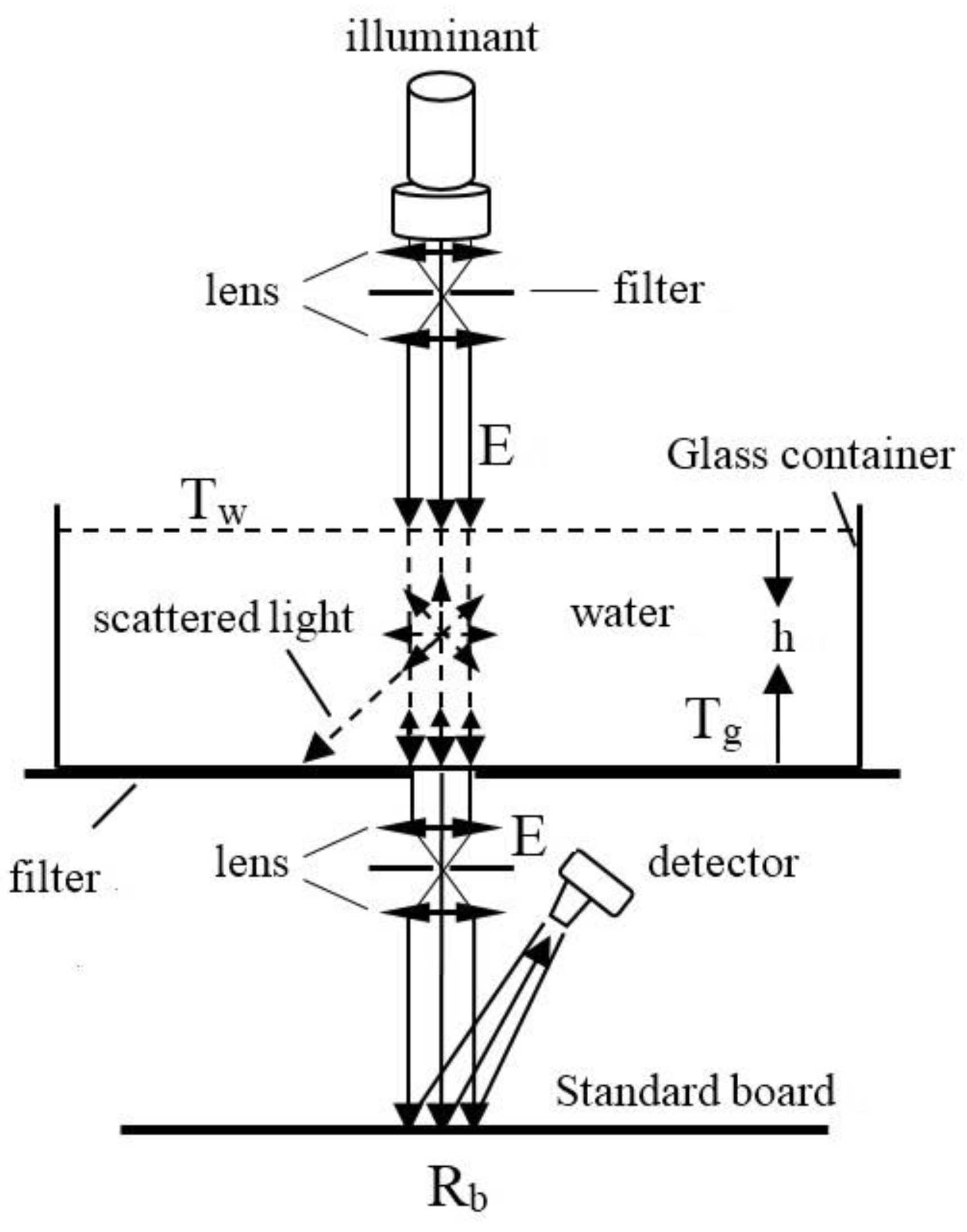
2.3.4. Optical Parameters Measurement of Organic Matter

The optical parameters of organic matter were measured using the method proposed by He [31]. The schematic diagram of the measuring device is shown in Figure 6. During the measurement, the light from a 65w constant light source passes through a set of lenses and filters to form a beam of parallel light that enters a certain height of the water sample to be measured in a high-transmittance glass container. After the parallel light passes through the bottom of the glass container, the downward scattered light is filtered by another group of lenses and filters, and the downward parallel light is irradiated onto the standard board. The radiance of the downward parallel light is measured by a spectrometer (ASD FieldSpec3 spectrometer manufactured by the U.S. Company ASD). The whole set of devices is installed in a closed multi-layer black cabinet, and the experiment is performed in a completely dark indoor environment, which makes the environment of each experiment almost unchanged and reduces the influence of external environmental factors.

The radiance detected by the spectrometer shown in Figure 6 as follows:

$$L=\frac{1}{\pi }{D}_{path}E{T}_w{e}^{-\tau }{T}_g{R}_b$$

(24)

where $D_{path}$is the path attenuation factor, i.e., the proportion of the irradiance of the incident light decreasing with the increase of the distance, $E$is the irradiance of the incident light source, $T_w$, $T_g$are the transmittance of the water surface and the bottom of the glass container, respectively, $R_b$ is the reflectance of the standard board, $e^{-\tau }$ is the transmittance of the water layer to be measured, and $\tau$is the optical thickness of the water layer:

$$\tau =d*k$$

(25)

where $d$ is the thickness of the water layer and $k$ is the extinction coefficient of the measured water body.

Equation (24) contains multiple unknown parameters. In order to eliminate systematic errors and avoid directly calculating $T_w$ and$T_g$, the ratio method is used to solve the extinction coefficient. The concentration of high organic pollution water collected in the field is a certain value. During measurement, the radiance of water bodies of different thicknesses is obtained by changing the thickness of the water body, and then the extinction coefficient of the water body is obtained by comparing the radiance information of different thicknesses. The ratio of the radiance $L_1$and $L_2$ measured by two water layers with different thicknesses $d_1$and $d_2$is as follows:

$$\frac{L_1}{L_2}=\frac{\frac{1}{\pi }{D}_{path}E{T}_w{e}^{-d_{1}k}{T}_g{R}_b}{\frac{1}{\pi }{D}_{path}E{T}_w{e}^{-d_{2}k}{T}_g{R}_b}$$

(26)

Equation (26) is sorted as follows.

$$k=\frac{1}{d_2-d_1}\ln \left(\frac{L_1}{L_2}\right)$$

(27)

In Equation (27),$L_1$ and $L_2$are directly measured by the spectrometer while$d_1$ and $d_2$can be accurately measured in the experiment. Thereby, the extinction coefficient $k$ of the measured water body can be calculated.

For a typical organic polluted water body, the total extinction coefficient$k_{total}={\alpha }_{total}+b_{btotal}$, which is measured in the laboratory, includes the contributions of various water components such as suspended sediment, chlorophyll, organic matter, and pure water. By substituting the total extinction coefficient $k_{total}$ into Equation (4), the total scattering coefficient $b_{btotal}$ can be obtained.

$$b_{btotal}=\frac{k_{total}*R_{rs}}{f}$$

(28)

In Equation (28), the water leaving reflectance $R_{rs}$of the water body was obtained through a simultaneous measurement by spectrometer during field sampling, and the total extinction coefficient $k_{total}$ of the water body was calculated by Equation (27) after conducting a measurement of the water sample collected from the field in the laboratory. Then, the total absorption coefficient ${\alpha }_{total}$of the water sample is shown below.

$${\alpha }_{total}=k_{total}-b_{btotal}$$

(29)

After the concentration of each component $C_{comp}$of the water body (subscript comp: c, s, and o represents Chl, SS, and organic matter) obtained through water sample analysis, the absorption coefficient ${\alpha }_o$ and backscatter coefficient $b_{bo}$ of the organic matter in the water sample can be obtained from Equations (5) and (6).

$${\alpha }_o=\frac{{\alpha }_{total}-\left({\alpha }_w+C_c{\alpha }_c+C_s{\alpha }_s\right)}{C_o}$$

(30)

$$b_{bo}=\frac{b_{btotal}-\left(b_{bw}+C_c{b}_{bc}+C_s{b}_{bs}\right)}{C_o}$$

(31)

2.3.5. Model Verification and Error Analysis

The accuracy of the retrieval model can be evaluated by calculating the mean absolute percentage error (MAPE) using the following equation [48].

$$MAPE=\frac{1}{n}{{\displaystyle \sum }}_{j=1}^n\left|\frac{C_j^{\prime }-C_j}{C_j}\right|*100\%$$

(32)

where $n$ is the number of the in situ measured samples, $C_j^{\prime }$ and $C_j$ are the retrieved value and the measured value of the concentration of the relevant water quality component of the $j^{th}$ sample.

3. Results

3.1. Water Quality Analysis Results and Measured Spectrum

3.1.1. Water Quality Analysis Results

The water quality analysis results of the water samples collected at each sampling site in the Pearl River channel experiment are shown in

Table 3. Water quality analysis results for each sampling site.

Sampling Sites	Longitude	Latitude	CODMn (mg/L)	Chla (μg/L)	SS (mg/L)	TP (mg/L)
A1	113.48527E	23.06805N	3.6	37.3	13	0.2
A2	113.46309E	23.08804N	4.8	40.3	32	0.32
A3	113.43014E	23.09443N	4.5	93.2	10	0.25
A4	113.40438E	23.10433N	5.6	83.2	35	0.4
A5	113.38273E	23.11063N	7	70.3	50	0.36
A6	113.35436E	23.10951N	5.2	57.8	22	0.26
A7	113.31902E	23.11102N	4.7	55.9	22	0.23
A8	113.27800E	23.11368N	5.7	95.5	11	0.25
A9	113.26353E	23.11598N	6.4	100	16	0.28
A10	113.24763E	23.10958N	6.7	94.7	15	0.27
A11	113.23928E	23.10695N	7.2	93.2	14	0.28
A12	113.22384E	23.11511N	6.4	93.2	14	0.28
A13	113.22289E	23.13993N	7.2	83.2	21	0.38
A14	113.21097E	23.15210N	7.2	70.3	30	0.37
B1	113.23506E	23.10697N	5.5	81	10	0.22
B2	113.25994E	23.06813N	3.7	31.1	9	0.13
B3	113.29135E	23.05522N	2.8	16.3	11	0.13
B4	113.32910E	23.04997N	2.8	16.7	8	0.11
B5	113.36762E	23.03687N	3	20.1	9	0.12
B6	113.41188E	23.05005N	2.9	14	8	0.12
B7	113.43564E	23.07768N	3.3	16	12	0.12

. The analysis results show that, among the 21 sampling sites in the simultaneous measurement of the Pearl River channels in Guangzhou, compared with B3-B7 sampling sites in the east part of the back channel, the concentration values of the water quality components in the A1-A14, B1, and B2 sampling sites in the front channel, the west channel, and the west part of the back channel are much higher, among which the concentration differences of Chl and permanganate index (COD_Mn) are the most clear. The concentrations of Chla and permanganate index of A1-A14, B1, and B2 sampling sites were higher than 30 μg/L and 3.5 mg/L, respectively, while those of B3-B7 were lower than 21 μg/L and 3.4 mg/L, respectively.

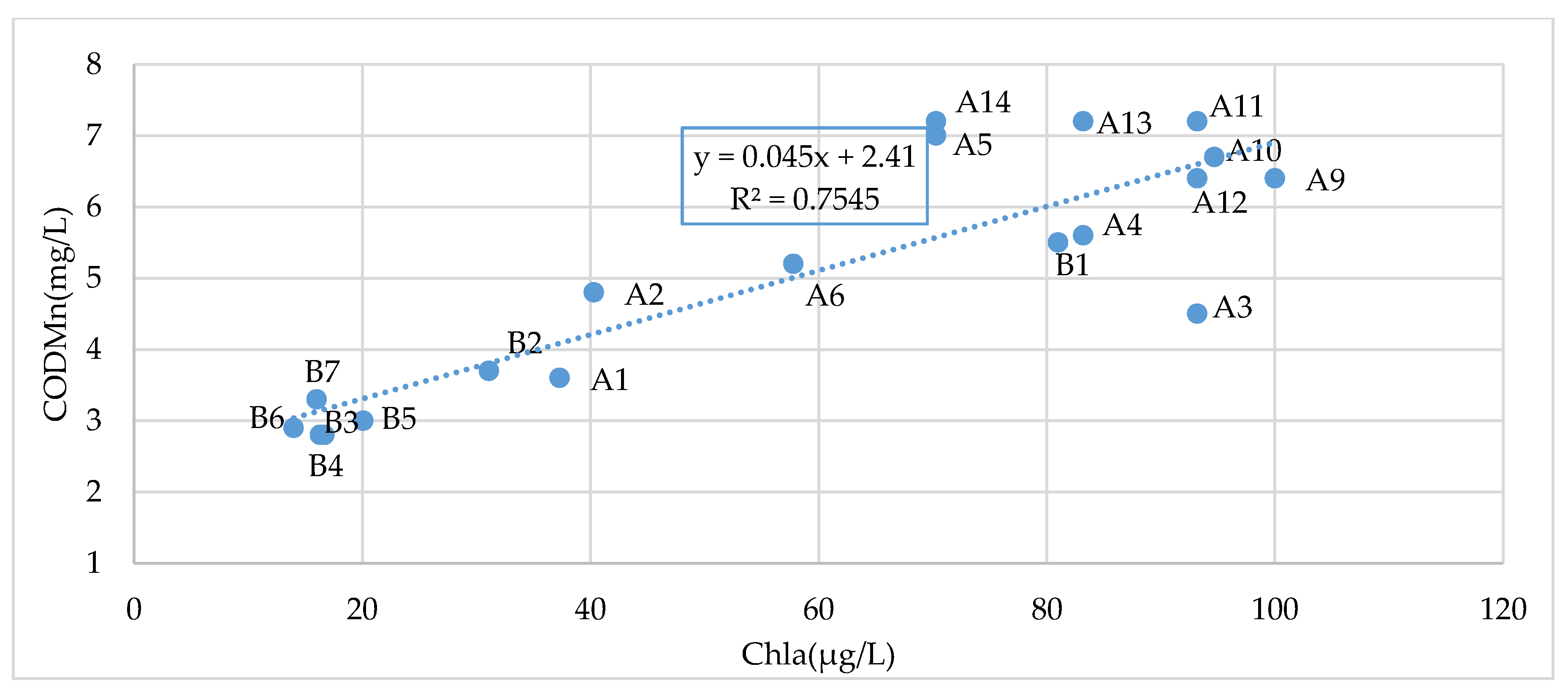
3.1.2. IOPs of Organic Matter in the Pearl River Channels in Guangzhou

For the typical organic polluted water samples collected from the Pearl River channels in Guangzhou, the absorption coefficient and backscatter coefficient of organic matter calculated by Equations (30) and (31) are shown in Figure 7 after using the water leaving reflectance measured during sampling. The water quality analysis results and the extinction coefficient were measured in the laboratory. The scattering coefficient of organic matter is very low compared with its absorption coefficient, and its absorption spectrum decays exponentially with the increase of the wavelength. The absorption of organic matter includes the absorption of dissolved organic matter and the absorption of suspended organic particles, which has a strong absorption effect on visible light. Therefore, the reflectance of heavily organic polluted water is very low, and the water appears black.

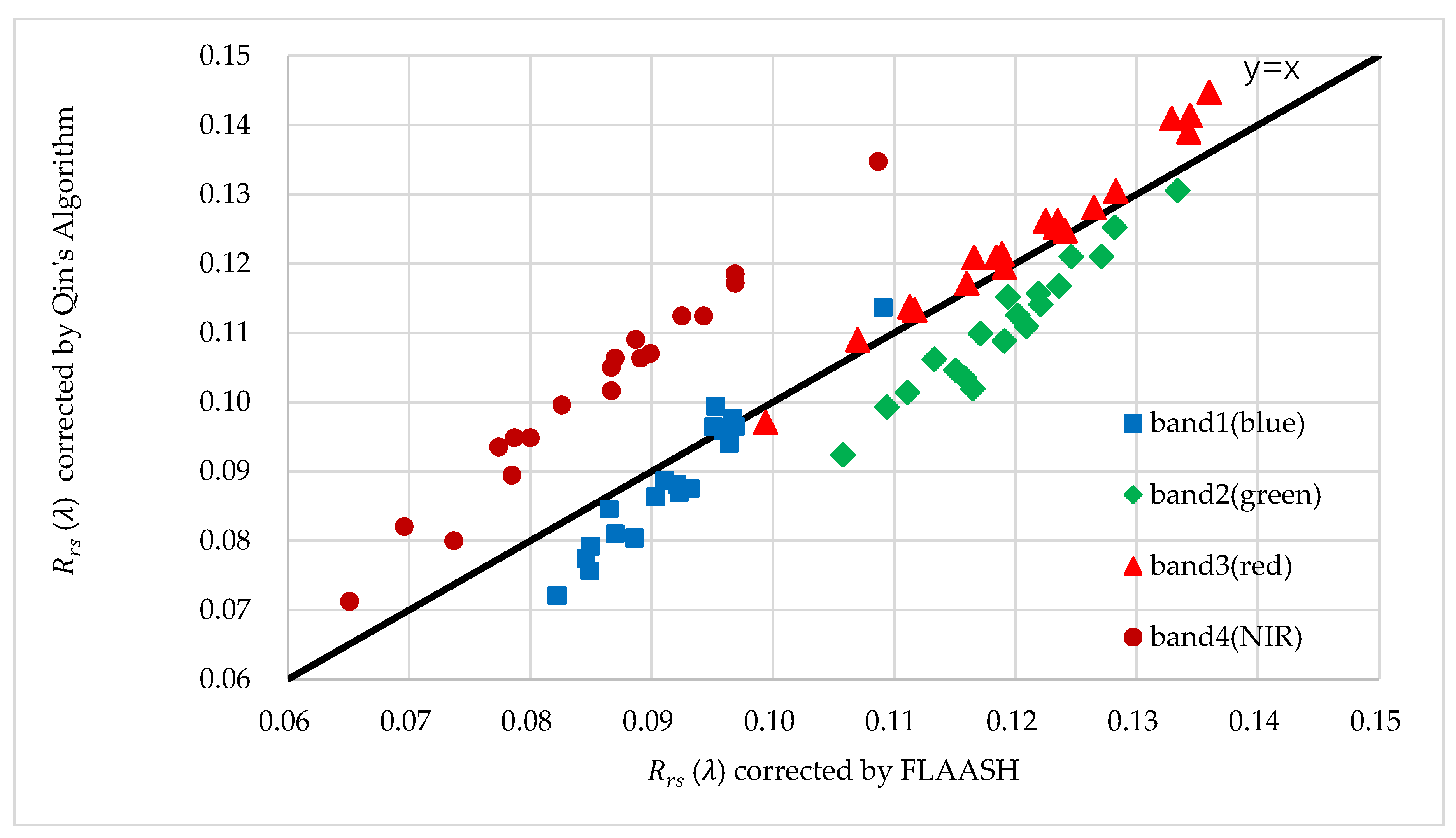
3.1.3. Measured Water Leaving Reflectance

Figure 8 shows the water leaving reflectance curves of the waters at the sampling sites in the Pearl River channel experiment on 5-6 August 2015. The figure shows the measured water leaving reflectance spectra in a wavelength ranging from 400 to 900 nm at each sampling site because the direct sunlight is blocked by the clouds. No measured spectra were obtained for the sampling sites of A7 and A8. As shown in

Table A1. The integral value of measured water leaving reflectance of GF-1 multispectral bands.

Sampling Sites	Integral Value of Measured Water Leaving Reflectance
	band1	band2	band3	band4
A1	0.04064	0.06152	0.05667	0.01759
A2	0.03656	0.06358	0.05995	0.01702
A3	0.03079	0.05039	0.03994	0.01003
A4	0.03220	0.05427	0.05264	0.02059
A5	0.03412	0.05628	0.05765	0.02996
A6	0.03873	0.06205	0.05350	0.01857
A9	0.05585	0.08819	0.05753	0.02525
A10	0.03671	0.05863	0.03938	0.01090
A11	0.03018	0.05501	0.03781	0.01133
A12	0.02930	0.04644	0.03401	0.00835
A13	0.03937	0.06086	0.05056	0.02361
A14	0.03048	0.05200	0.04170	0.01420
B1	0.02568	0.04692	0.03729	0.01070
B2	0.03566	0.06258	0.05010	0.01017
B3	0.03319	0.05866	0.05566	0.01121
B4	0.04270	0.07186	0.05841	0.00809
B5	0.04354	0.07140	0.06928	0.01715
B6	0.05271	0.08434	0.06819	0.01068
B7	0.05030	0.08101	0.07788	0.01944

, by using the GF-1 satellite spectral response function [49], the measured water leaving reflectance spectra are integrated to obtain the water leaving reflectance values, which correspond to the four GF-1 spectral bands at each sampling site. As shown in Figure 8, for the water samples with a high concentration of Chla and COD_Mn, A1-A14, B1, and B2, there is a clear reflection valley near 670 nm and a clear reflection peak near 700 nm, which corresponds to the absorption peak near 670 nm of the Chla absorption coefficient curve and the absorption valley near 700 nm of the absorption coefficient curve of organic matter. For B3-B7, water samples with low Chla and COD_Mn concentrations, their spectral curves did not have clear absorption valleys and absorption peaks around 670 nm and 700 nm.

3.2. Verification of the TP Inversion Model

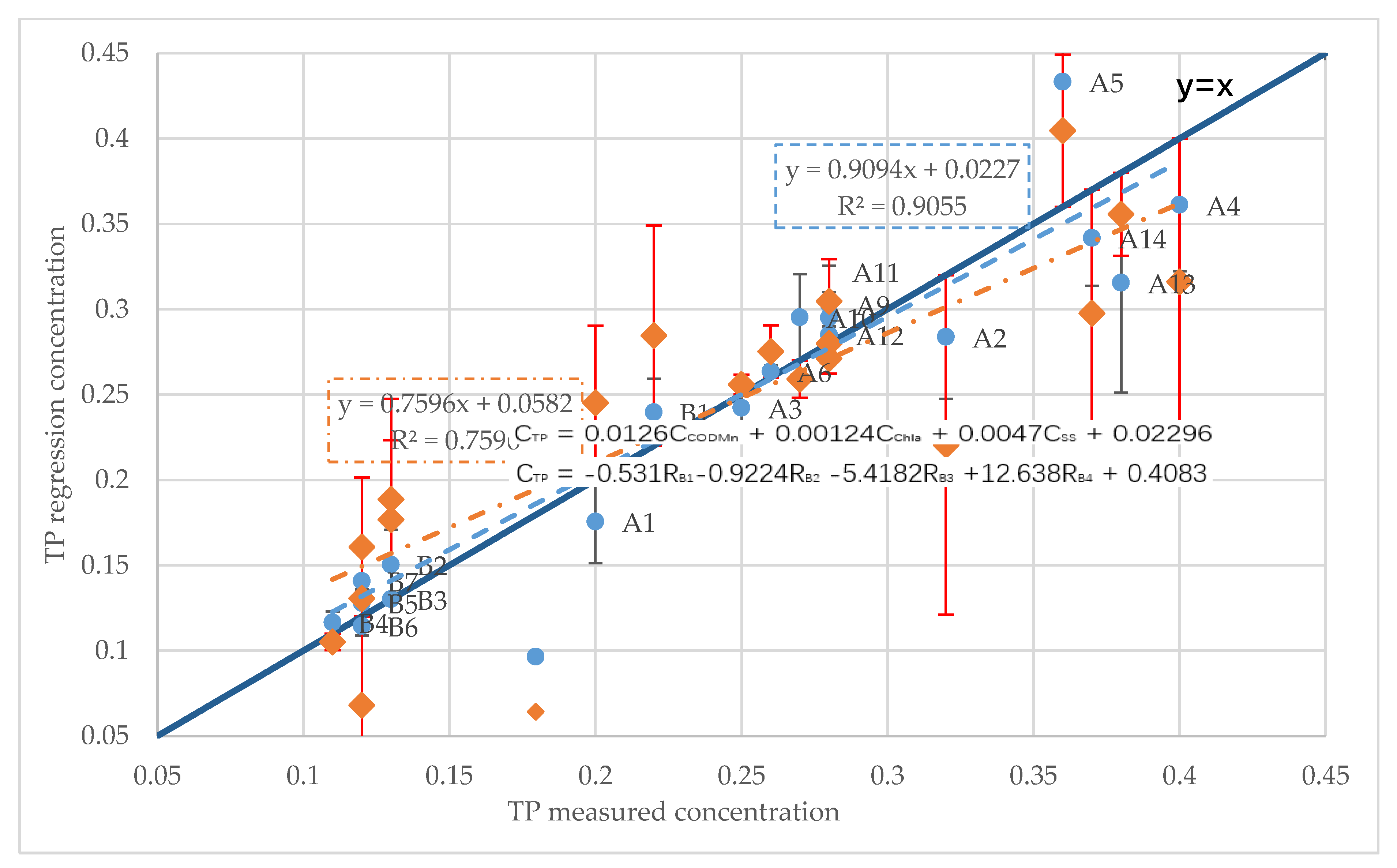
3.2.1. TP Inversion Model

The regression of TP concentration in the Pearl River channel in Guangzhou with the water sample quality analysis results and the measured spectral data are shown in

Table 4. Regression analysis of total phosphorus (TP) and other water quality parameters.

Water Quality Parameters	Regression Equations	R2	F
CODMn	CTP= 0.05063X − 0.0132	0.7437	49.333
Chla	CTP = 0.00228X + 0.10855	0.5636	21.953
SS	CTP = 0.00672X + 0.12229	0.5974	25.225
CODMn + Chla	CTP = 0.05029X1 + 0.000002X2 − 0.01264	0.7437	23.217
CODMn + SS	CTP = 0.03682X1 + 0.00373X2 − 0.01009	0.8727	54.828
Chla + SS	CTP = 0.00174X1 + 0.005258X2 + 0.0462	0.8985	70.823
CODMn + Chla + SS	CTP = 0.0126X1 + 0.00124X2 + 0.0047X3 + 0.02296	0.9055	47.886

and

Table 5. Regression analysis of TP and the measured water leaving reflectance (R² > 0.3).

GF-1 Wavebands	Regression Equations	R2	F
B1, B4	CTP = −7.4893RB1 + 10.90179RB4 + 0.35623	0.5877	11.405
B2, B4	CTP = −5.27644RB2 + 10.34687RB4 + 0.4109	0.6215	13.135
B3, B4	CTP = −6.46467RB3 + 12.76875RB4 + 0.38358	0.7507	24.084
B1, B2, B3	CTP = 15.1327RB1 − 12.7831RB2 − 1.57399RB3 + 0.5503	0.3121	2.2681
B1, B2, B4	CTP = 3.9819RB1 − 7.8961RB2 + 9.5857RB4 + 0.42982	0.6259	8.3647
B1, B3, B4	CTP = −1.7354RB1 − 5.5486RB3 + 12.7926RB4 + 0.40073	0.7592	15.764
B2, B3, B4	CTP = −1.2906RB2 − 5.3924RB3 + 12.5756RB4 + 0.4108	0.7595	15.794
B1, B2, B3, B4	CTP = −0.531RB1 − 0.9224RB2 − 5.4182RB3 + 12.638RB4 + 0.4083	0.7596	11.06

. In the regression analysis of various combinations of water sample quality parameters, which are shown in Table 4, the correlation coefficient between TP concentration and a combination of COD_Mn, Chla, and SS is the highest (R² = 0.9055, F value for F-test = 47.886). Similarly, in the regression analysis of various combinations of measured spectral data shown in Table 5, the correlation coefficient between TP concentration and a combination of four bands is the highest (R² = 0.7596, F value for F-test = 11.06). The two regression equations with the highest correlation in Table 4 and Table 5 are used to calculate the TP concentration of 19 sampling sites in Table 3 (excluding A7 and A8). The results are shown in Figure 9. The MAPE of the combination of COD_Mn, Chla, and SS is 8.77%, which is better than that of the combination of four bands (the MAPE is 17.8%).

3.2.2. Inversion Results Based on Measured Data

Figure 10 shows the retrieved concentration from the in situ measured spectra, measured concentration, and relative retrieval errors of TP, COD_Mn, SS, and Chla at the 19 sampling sites. First, by using the GF-1 satellite spectral response function, the measured spectra are integrated to obtain the water leaving reflectance values, which correspond to the four GF-1 spectral bands at each sampling site (Table A1). Using Equations (22) and (23), the concentration of the relevant water quality components is obtained, and the relative retrieval error at each sampling site and MAPE of the model are calculated. For the in situ measured data, the MAPEs of the retrieved concentrations TP, COD_Mn, SS, and Chla relative to the measured values are 17.98%, 30.98%, 54.06%, and 51.2%, respectively.

3.3. Remote Sensing Retrieval of Water Quality Parameters in the Pearl River Channels

3.3.1. Water Leaving Reflectance of Remote Sensing Data

The remote sensing retrieval process of TP in the Pearl River Channels is shown in Figure 3. By using Equation (1), radiometric calibration of the GF-1 multispectral remote sensing data was performed to convert the satellite-based observation values into radiance. Then, an image-based automatic inversion algorithm of aerosol optical density proposed by Qin et al. (2015) was used for atmospheric correction. First, partition the entire image to select the dark pixels of shady vegetation, and estimate the phase function and scattering ratio of aerosol in the red and blue channels based on the path radiance. Second, on the basis of Gilabert’s algorithm [50], the consideration of diffuse reflection on the surface is added, and the simplified radiative transfer equation is used to calculate the aerosol optical density of shading vegetation and dense vegetation dark pixels. Lastly, Kriging interpolation is used to calculate the aerosol optical density of multiple dark image elements for the distribution of the entire scene image, and then an atmospheric correction is carried out. The remote sensing water leaving reflectance corresponding to each sampling site is shown in Figure 11 and

Table A2. The remote sensing reflectance of GF-1 image corresponding to sampling sites.

Sampling Sites	Remote Sensing Reflectance of GF-1 Image
	band1	band2	band3	band4
A1	0.07740	0.10619	0.120927	0.07999
A2	0.0756208	0.101952	0.12474	0.0894474
A3	0.07205	0.09242	0.09709	0.0711984
A4	0.080971	0.103542	0.121404	0.109048
A5	0.0881046	0.115195	0.130462	0.118511
A6	0.0791876	0.101423	0.11330	0.0948545
A9	0.0845378	0.09930	0.109008	0.101613
A10	0.09762	0.11096	0.12617	0.11716
A11	0.0940492	0.109898	0.120927	0.106345
A12	0.0993994	0.114135	0.119497	0.107021
A13	0.088699	0.104601	0.11378	0.112428
A14	0.0964271	0.112546	0.11711	0.104993
B1	0.0964271	0.116784	0.12617	0.112428
B2	0.113666	0.13056	0.14476	0.134732
B3	0.0958326	0.12526	0.14095	0.09350
B4	0.0863212	0.115725	0.12522	0.0820126
B5	0.08692	0.121022	0.139043	0.0995858
B6	0.0875101	0.121022	0.141427	0.106345
B7	0.08038	0.10884	0.12808	0.09485

. As an example, Figure 12 shows the water leaving reflectance curves of the A1 sampling site. According to the atmospheric correction results, the Qin’s algorithm is similar to the Fast Line-of-Sight Atmospheric Analysis of Hypercubes (FLAASH) algorithm. In the blue and green bands, the water leaving reflectance of Qin’s algorithm is slightly lower than the FLAASH algorithm, while, in the red and near-infrared bands, it is the opposite. The water leaving reflectance of the algorithm is higher than that of the FLAASH algorithm. Compared with the measured water leaving reflectance, the results of the two atmospheric correction algorithms are higher than the measured values. Except for the green band, the MAPE of the other bands exceeds 100%, especially in the near infrared band. The MAPE of the two algorithms are more than 500%.

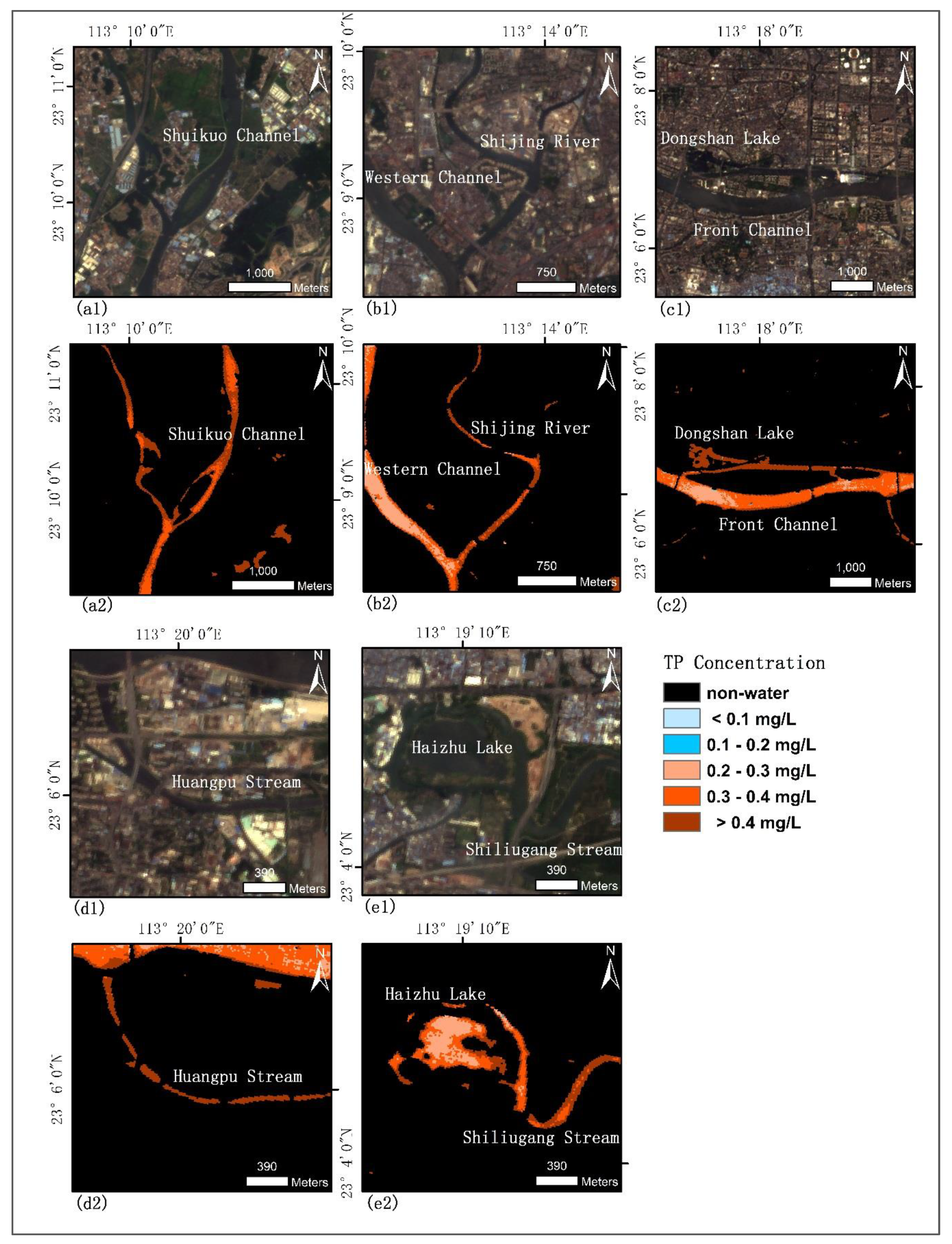
3.3.2. Remote Sensing Retrieval Result of TP in the Pearl River Channels

By substituting the remote sensing water leaving reflectance of the three bands of water pixels and the IOPs of each water quality component in Equations (22) and (23), the TP concentration of each water pixel is retrieved (Figure 13). The details of five areas with high TP concentration indicated in Figure 13a are shown in Figure 14.

Figure 15 shows the retrieved concentration from the GF-1 remote sensing data, measured concentration, and relative retrieval errors of TP, COD_Mn, SS, and Chla at the 19 sampling sites. First, by using the geographical coordinates of each sampling site, the remote sensing water leaving reflectance of each band corresponding to each pixel of sampling sites is extracted from the GF-1 remote sensing image (Table A2). Second, using Equations (22) and (23), the concentration of the relevant water quality components is obtained, and the relative retrieval error at each sampling site and MAPE of the model are calculated. For the GF-1 remote sensing data, the MAPEs of the retrieved concentrations TP, COD_Mn, SS, and Chla are 24.18%, 31.45%, 42.21%, and 71.99%, respectively.

Figure 13a shows the inversion results on 7 August 2015. The MAPE is 24.18% based on the measured values. The retrieval results show that the TP concentration of most waters in the Front Channel, Western Channel, Guanzhou Channel, and western part of the Back Channel of the Pearl River is larger than 0.2 mg/L. The TP concentration of waters in the east part of the Back Channel is primarily less than 0.2 mg/L. This concentration distribution is attributed to the notion that the Western Channel and the western parts of the Front and Back Channels are administered by the Baiyun District of Guangzhou and Foshan City (Figure 14a1,a2,b1,b2), while the middle part of the Front Channel and Guanzhou Channel are located in Guangzhou’s downtown area (Figure 14c1,c2,d1,d2,e1,e2). There are numerous industrial enterprises and a dense urban population around these areas. Industrial pollution, and urban sewage increase the TP concentration of these waters. There are also some vegetable planting areas around the Shuikou Channel and Shiliugang Stream. The phosphorus emission caused by fertilization may also be one of the reasons for the high concentration of TP in these two areas. The possibility of the increase of the TP concentration in the water body caused by such fertilization is based on the fact that, at present, in the vegetable planting in South China, almost no vegetable growers will carry out "soil testing and formula fertilization." Over fertilization is a common phenomenon. Moreover, in Guangzhou, the temperature is very high in August, so the vegetable planting must be frequently watered to ensure the normal growth of vegetables, but part of the phosphorus in the artificial fertilizer will also be leached and lost due to watering and enter the nearby water body. Due to the dilution effect of the Sanzhixiang channel with low TP concentration, the TP concentration of waters in the middle and rear part of the back channel is relatively low. The TP retrieval’s statistical results show that the TP concentration of most waters (approximately 66%) of the Pearl River channels in Guangzhou ranges between 0.1 mg/L and 0.3 mg/L, and the TP concentration of approximately 32% of the waters is larger than 0.3 mg/L.

Figure 13b shows the inversion results on 24 October 2015. The results show that the TP concentration in most water bodies of the Pearl River channels in Guangzhou at the time of imaging is greater than 0.4 mg/L. Because there are no synchronized measured values, the inversion accuracy evaluation corresponding to the water quality monitoring data of Guangzhou in October 2015 queried in the Guangzhou Environmental Protection Geographic Information System was used [51]. The MAPE was 22.34%.

4. Discussion

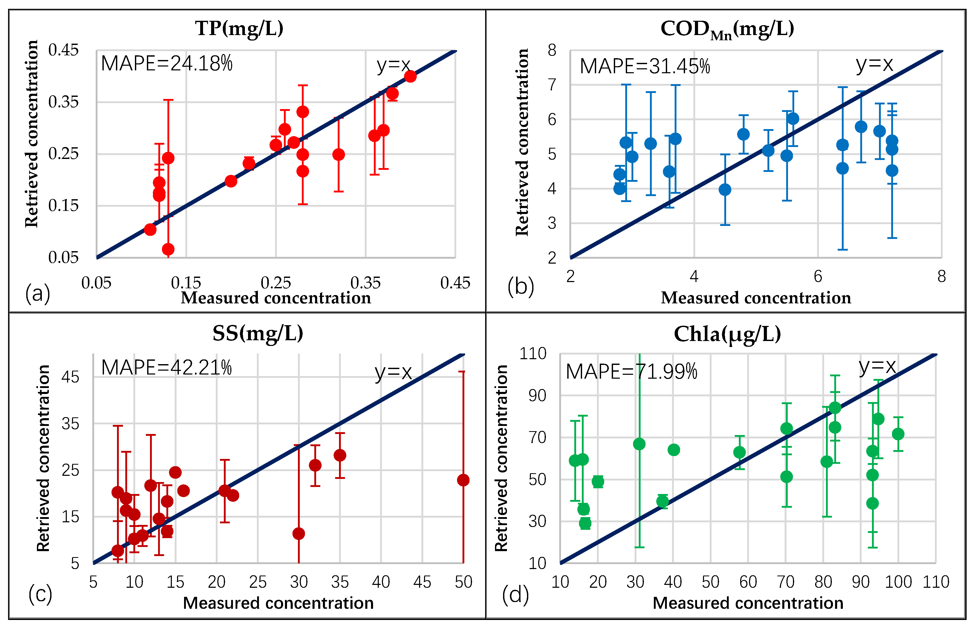
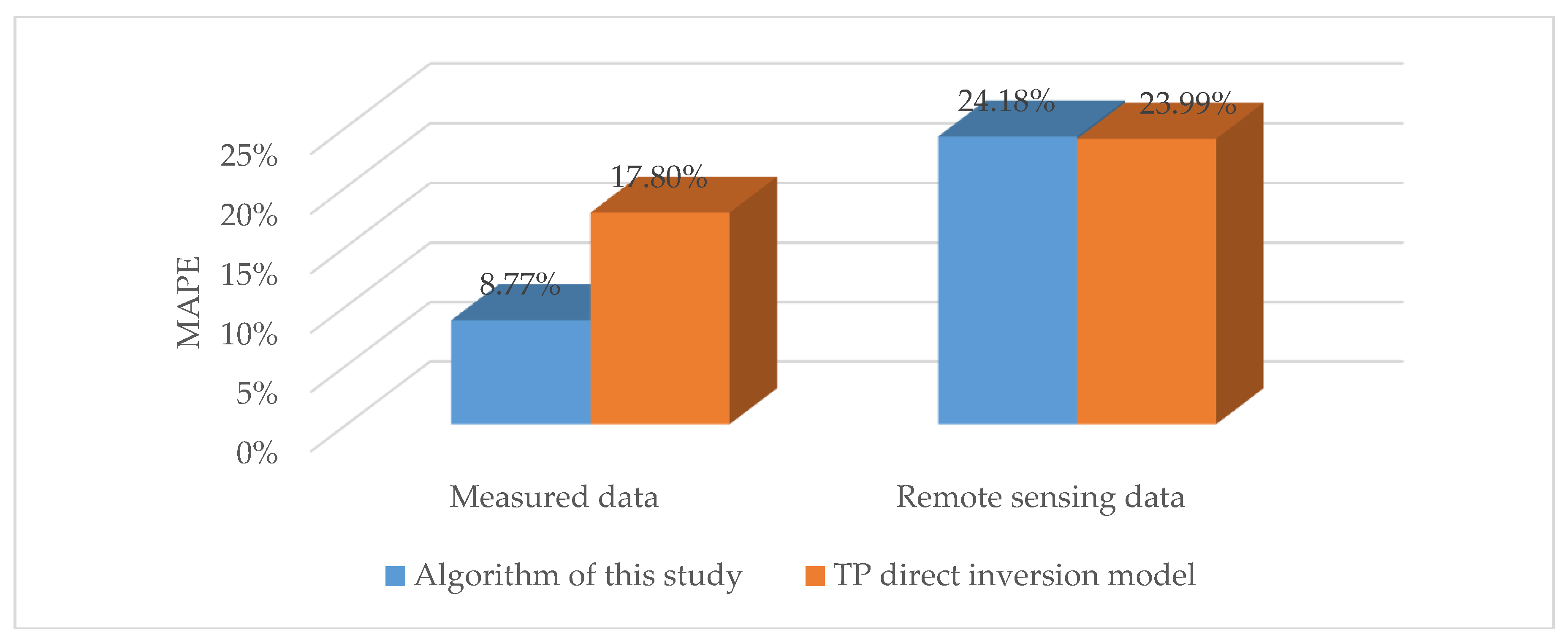
4.1. Error Analysis of the Retrieval Results

The retrieval error analysis of the model is shown in Figure 16. The retrieval of TP is affected by a combined effect of Chla, SS, and COD_Mn, but is insensitive to the retrieval accuracy of the individual components. As shown in Figure 16, when the inversion error of any water quality component in Chla, SS, and COD_Mn increases to 60% or 70%, or the inversion error of any two components exceeds ± 35%, or the inversion error of three components exceeds ± 20%, the MAPE of TP will increase from 8.7% to 20%. Therefore, as shown in Figure 10 and Figure 15, when the retrieval MAPE of Chla, SS, and COD_Mn change by 20.79%, 11.85%, and 0.47%, respectively, the MAPE of TP increases by 6.38%. The relative errors of Chla, COD_Mn, and TP retrieved from the remote sensing data were larger than those of the in situ measured data, among which the retrieved errors of Chla at B2-B7 sites are all more than 100%, which produces a sharp increase in the retrieval of the MAPE of Chla. When B2-B7 are disregarded, the MAPE of Chla based on the in situ measured data and the GF-1 remote sensing data decreases to 19.18% and 25.01%, respectively. It is found that the measured concentrations of Chla, SS, and COD_Mn in B2-B7 sites are much lower than those in other sites in Table 3. However, the comprehensive inversion coefficient introduced in this study will overestimate the concentration of water components in the site with low measured concentration (Figure 10 and Figure 15), which makes the relative retrieval errors of the site with low measured concentration become larger. How to improve the inversion accuracy of water with low concentration of Chla and SS needs further study.

4.2. Applicability of the Model

Figure 13a,b show the results of TP inversion of the Pearl River channels in Guangzhou by GF-1 remote sensing image with imaging time of 7 August 2015 and 24 October 2015, respectively. It can be seen from the figure that, on 24 October 2015, the TP concentration of the Pearl River channels in Guangzhou was mostly higher than 0.4 mg/L, while on 7 August 2015, the TP concentration was relatively low, with the concentration of most water bodies less than 0.4 mg/L. This is because August is the wet season of the Pearl River. The replenishment of a large number of clean water bodies in the main stream of the Pearl River, Xijiang River, and Beijiang River has diluted the TP concentration of the water body. However, October has entered the normal water period, and the replenishment of clean water bodies in the middle and upper reaches has been continuously reduced and the dilution effect has been weakened, so that the TP concentration in the water body of the Pearl River channels in Guangzhou remains at a high level.

As shown in Figure 17, compared with the TP inversion model established by directly using the reflectance of four bands, the inversion accuracy of the TP indirect inversion model proposed in this study is higher, and COD_Mn, which is another water quality index for the surface water environmental quality assessment, can also be obtained by inversion. The TP indirect inversion model is an empirical inversion model based on the measured data of the water body in the Pearl River channels in Guangzhou. This kind of model is usually only applicable to specific water bodies. When applying it to other types of water bodies, the measured data should be used for model calibration to obtain appropriate inversion parameters. According to the analysis results of Zheng et al. (2016), the proportion of the dissolved organic matter (DOM) in the water bodies of the Pearl River channels in Guangzhou in different seasons is somewhat similar. The category of DOM in the water bodies does not change much, except that the concentration is low in the summer during the wet season. Therefore, it is feasible to use this model to retrieve the TP concentration in the water bodies of the Pearl River channels in Guangzhou in different seasons. The water quality analysis results of each sampling site used to build the model in this study show that the concentration of Chla has a high correlation with the concentration of COD_Mn (R² = 0.75), but the concentration distribution is uneven, which accounts for 52.63% of Chla > 70 μg/L and COD_Mn > 4.5 mg/L, 36.84% of Chla < 40 μg/L and COD_Mn < 4 mg/L. The number of samples with medium concentration distribution is small, with only A2 and A6, which accounts for 10.53% (Figure 18). It can be seen that the inversion error of Chla and COD_Mn for low-concentration water bodies in the model constructed from these samples will be higher, which, thereby, increases the TP inversion error (Figure 10 and Figure 16). In the following work, attention should be paid to the reasonable selection of sampling sites and the study of constructing the TP inversion model, according to the concentration distribution of water quality components.

It can be seen from Figure 10 and Figure 11 that the atmospheric correction algorithm used in this paper is similar to the FLAASH algorithm in atmospheric correction, and the corrected water leaving reflectance is very different from the measured value. Although Qin et al. applications of this algorithm have achieved good results in retrieving the aerosol optical thickness of Hong Kong, China using the multispectral remote sensing image of Ziyuan-3 [18], to be successfully applied to GF-1 remote sensing image, the selection of dark pixels and the inversion algorithm of aerosol optical thickness in urban areas need to be further optimized.

5. Conclusions

TP concentration is one of the indicators for surface water quality evaluation. In this study, an indirect retrieval algorithm for TP concentration was proposed. Based on the GF-1 remote sensing data, the TP concentration in urban waters was retrieved. The algorithm establishes a retrieval model that is based on the relationship among remote-sensing reflectance, optically significant constituents of water (chlorophyll, SS, organic matter), and TP. First, the concentration of optically active components was obtained by retrieval analysis using a semi-analytical model. Second, the TP concentration of waters is retrieved by using the correlation between TP and optically active components. The retrieval results of TP using GF-1 remote-sensing water leaving reflectance on 7 August 2015 illustrated the distribution of TP concentration in the Pearl River channels in Guangzhou on this day. The TP concentration of most waters in the Front Channel, the Western Channel, the Guanzhou Channel, and the western part of the Back Channel of the Pearl River was larger than 0.2 mg/L. The TP concentration of waters in the east part of the back channel was generally less than 0.2 mg/L. Using TP concentration as an evaluation index, most waters in Guangzhou’s river channels are classified as Class III and Class IV water bodies, according to the Environmental Quality Standards for Surface Water (GB 3838-2002). These waters satisfy the standards for general industrial water and entertainment water, which does not directly contact human bodies. The retrieval MAPE of TP concentration is 24.18%. This model is suitable for the retrieval of TP concentration in Guangzhou’s urban waters.

References

1. Gulati, R.D.; Van Donk, E. Lakes in the Netherlands, their origin, eutrophication and restoration: State-of-the-art review. Hydrobiologia 2002, 478, 73–106. [Google Scholar] [CrossRef]
2. Sileika, A.S.; Wallin, M.; Gaigalis, K. Assessment of nitrogen pollution reduction options in the river Nemunas (Lithuania) using FyrisNP model. J. Environ. Eng. Landsc. Manag. 2012, 21, 141–151. [Google Scholar] [CrossRef]
3. Zafar, M.; Tiecher, T.; de Castro Lima, J.A.M.; Schaefer, G.L.; Santanna, M.A.; Dos Santos, D.R. Phosphorus seasonal sorption-desorption kinetics in suspended sediment in response to land use and management in the Guaporé Catchment, Southern Brazil. Environ. Monit. Assess. 2016, 188, 643. [Google Scholar] [CrossRef]
4. Li, Y.; Zhang, Y.; Shi, K.; Zhu, G.; Zhou, Y.; Zhang, Y.; Guo, Y. Monitoring spatiotemporal variations in nutrients in a large drinking water reservoir and their relationships with hydrological and meteorological conditions based on Landsat 8 imagery. Sci. Total Environ. 2017, 599–600, 1705–1717. [Google Scholar] [CrossRef]
5. Wu, C.; Wu, J.; Qi, J.; Zhang, L.; Huang, H.; Lou, L.; Chen, Y. Empirical estimation of total phosphorus concentration in the mainstream of the Qiantang River in China using Landsat TM data. Int. J. Remote Sens. 2010, 31, 2309–2324. [Google Scholar] [CrossRef]
6. Gao, Y.; Gao, J.; Yin, H.; Liu, C.; Xia, T.; Wang, J.; Huang, Q. Remote sensing estimation of the total phosphorus concentration in a large lake using band combinations and regional multivariate statistical modeling techniques. J. Environ. Manag. 2015, 151, 33–43. [Google Scholar] [CrossRef]
7. Hui, J.; Yao, L. Analysis and inversion of the nutritional status of China’s Poyang lake using MODIS data. J. Indian Soc. Remote. Sens. 2016, 44, 837–842. [Google Scholar] [CrossRef]
8. Huang, C.; Guo, Y.; Yang, H.; Li, Y.; Zou, J.; Zhang, M.; Lyu, H.; Zhu, A.; Huang, T. Using remote sensing to track variation in phosphorus and its interaction with chlorophyll-a and suspended sediment. IEEE J. Sel. Top. Appl. Earth Obs. Remote. Sens. 2015, 8, 4171–4180. [Google Scholar] [CrossRef]
9. Moses, S.A.; Janaki, L.; Joseph, S.; Kandathil, R.K. Determining the spatial variation of phosphorus in a lake system using remote sensing techniques. Lakes Reserv. Res. Manag. 2014, 19, 24–36. [Google Scholar] [CrossRef]
10. Goes, J.I.; Saino, T.; Oaku, H.; Jiang, D.L. A method for estimating sea surface nitrate concentrations from remotely sensed SST and chlorophyll a-a case study for the north Pacific Ocean using OCTS/ADEOS data. IEEE Trans. Geosci. Electron. 1999, 37, 1633–1644. [Google Scholar] [CrossRef]
11. Silió-Calzada, A.; Bricaud, A.; Gentili, B. Estimates of sea surface nitrate concentrations from sea surface temperature and chlorophyll concentration in upwelling areas: A case study for the Benguela system. Remote Sens. Environ. 2008, 112, 3173–3180. [Google Scholar] [CrossRef]
12. Baustian, J.J.; Kowalski, K.P.; Alex, C. Using turbidity measurements to estimate total phosphorus and sediment flux in a great lakes coastal wetland. Wetlands 2018, 38, 1059–1065. [Google Scholar] [CrossRef]
13. Guildford, S.J.; Hecky, R.E. Total nitrogen, total phosphorus, and nutrient limitation in lakes and oceans: Is there a common relationship? Limnol. Oceanogr. 2000, 45, 1213–1223. [Google Scholar] [CrossRef] [Green Version]
14. Tang, J.; Tian, G.; Wang, X.Y.; Wang, X.M.; Song, Q. The Methods of Water Spectra Measurement and Analysis Ⅰ: Above-Water Method. J. Remote Sens. 2004, 8, 37–44. [Google Scholar] [CrossRef]
15. Li, Z.; Shen, H.; Li, H.; Xia, G.; Gamba, P.; Zhang, L. Multi-feature combined cloud and cloud shadow detection in GF-1 WFV imagery. Remote Sens. Environ. 2016, 191, 342–358. [Google Scholar] [CrossRef] [Green Version]
16. China Centre for Resources Satellite Data and Application. Available online: http://218.247.138.119/CN/Satellite/3076.shtml (accessed on 15 October 2014).
17. China Centre for Resources Satellite Data and Application. Available online: http://218.247.138.119/CN/Downloads/dbcs/6709.shtml (accessed on 14 October 2015).
18. Qin, Y.; Deng, R.; He, Y.; Liu, X.; Liang, Y. Automatic retrieval of aerosol optical depth over Hong Kong using ZY-3 MUX. Acta Sci. Circum. 2015, 35, 1512–1519. [Google Scholar] [CrossRef]
19. Jiang, W.; He, G.; Long, T.; Ni, Y.; Liu, H.; Peng, Y.; Lu, K.; Wang, G. Multilayer Perceptron Neural Network for Surface Water Extraction in Landsat 8 OLI Satellite Images. Remote Sens. 2018, 10, 755. [Google Scholar] [CrossRef] [Green Version]
20. Lee, Z.; Carder, K.L.; Mobley, C.D.; Steward, R.G.; Patch, J.S. Hyperspectral remote sensing for shallow waters. 2. deriving bottom depths and water properties by optimization. Appl. Opt. 1999, 38, 31–43. [Google Scholar] [CrossRef] [Green Version]
21. Gordon, H.R.; Brown, O.B.; Evans, R.H.; Brown, J.W.; Smith, R.C.; Baker, K.S.; Clark, D.K. A semianalytic radiance model of ocean color. J. Geophys. Res. 1988, 93, 10909–10924. [Google Scholar] [CrossRef]
22. Lee, Z.P.; Carder, K.L.; Arnone, R.A. Deriving inherent optical properties from water color: A multiband quasi-analytical algorithm for optically deep waters. Appl. Opt. 2002, 41, 5755–5772. [Google Scholar] [CrossRef]
23. Wang, P.; Boss, E.S.; Roesler, C. Uncertainties of inherent optical properties obtained from semianalytical inversions of ocean color. Appl. Opt. 2005, 44, 4074–4085. [Google Scholar] [CrossRef]
24. Pegau, W.S.; Gray, D.; Zaneveld, J.R.V. Absorption and attenuation of visible and near-infrared light in water: Dependence on temperature and salinity. Appl. Opt. 1997, 36, 6035–6046. [Google Scholar] [CrossRef] [PubMed] [Green Version]
25. Pope, R.M.; Fry, E.S. Absorption spectrum (380–700 nm) of pure water. Ⅱ. Integrating cavity measurements. Appl. Opt. 1997, 36, 8710–8723. [Google Scholar] [CrossRef] [PubMed]
26. Volpe, V.; Silvestri, S.; Marani, M. Remote sensing retrieval of suspended sediment concentration in shallow waters. Remote Sens. Environ. 2011, 115, 44–54. [Google Scholar] [CrossRef]
27. Brando, V.E.; Dekker, A.G. Satellite hyperspectral remote sensing for estimating estuarine and coastal water quality. IEEE Trans. Geosci. Electron. 2003, 41, 1378–1387. [Google Scholar] [CrossRef]
28. Brando, V.E.; Anstee, J.M.; Wettle, M.; Dekker, A.G.; Phinn, S.R.; Roelfsema, C. A physics based retrieval and quality assessment of bathymetry from suboptimal hyperspectral data. Remote Sens. Environ. 2009, 113, 755–770. [Google Scholar] [CrossRef]
29. Gons, H.J.; Burger-Wiersma, T.; Otten, J.H.; Rijkeboer, M. Coupling of phytoplankton and detritus in a shallow, eutrophic lake (Lake Loosdrecht, the Netherlands). Hydrobiologia 1992, 233, 51–59. [Google Scholar] [CrossRef]
30. Deng, R.; He, Y.; Qin, Y.; Cheng, Q.; Cheng, L. Pure water absorption coefficient measurement after eliminating the impact of suspended substance in spectrum from 400 nm to 900 nm. J. Remote Sens. 2012, 16, 174–191. [Google Scholar]
31. He, Y.; Deng, R.; Cheng, Q.; Cheng, L.; Qin, Y. Diffuse Attenuation Coefficient of Suspended Sediment based on ASD Spectrometer. Acta Sci. Nat. Univ. Sunyatseni Nat. Sci. 2011, 50, 134–140. [Google Scholar]
32. Bricaud, A.; Morel, A.; Prieur, L. Absorption by dissolved organic matter of the sea (yellow substance) in the uv and visible domains. Limnol. Oceanogr. 1981, 26, 43–53. [Google Scholar] [CrossRef]
33. Kheireddine, M.; Ouhssain, M.; Calleja, M.L.; Morán, X.A.G.; Sarma, Y.; Tiwari, S.P.; Jones, B.H. Characterization of light absorption by chromophoric dissolved organic matter (CDOM) in the upper layer of the red sea. Deep Sea Res. Part. I Oceanogr. Res. Pap. 2018, 133, 72–84. [Google Scholar] [CrossRef] [Green Version]
34. Siegel, D.A.; Behrenfeld, M.J.; Maritorena, S.; Mcclain, C.R.; Antoine, D.; Bailey, S.W.; Bontempi, P.S.; Boss, E.S.; Dierssen, H.M.; Doney, S.C.; et al. Regional to global assessments of phytoplankton dynamics from the SeaWiFS mission. Remote Sens. Environ. 2013, 135, 77–91. [Google Scholar] [CrossRef] [Green Version]
35. Li, D.; Wu, H.; Huang, F.; Lin, X. Determination of Organic Compounds in Pear River Water by Gas Chromatography- Mass Spectrometry. J. Instrum. Anal. 2002, 21, 86–88. [Google Scholar]
36. Zheng, L.; Song, Z.; Meng, P.; Fang, Z. Seasonal characterization and identification of dissolved organic matter (DOM) in the pearl river, China. Environ. Sci. Pollut. Res. 2016, 23, 7462–7469. [Google Scholar] [CrossRef] [PubMed]
37. Rochelle-Newall, E.J.; Fisher, T.R. Chromophoric dissolved organic matter and dissolved organic carbon in Chesapeake Bay. Mar. Chem. 2002, 77, 23–41. [Google Scholar] [CrossRef]
38. Kowalczuk, P.; Cooper, W.J.; Whitehead, R.F.; Durako, M.J.; Sheldon, W. Characterization of CDOM in an organic-rich river and surrounding coastal ocean in the South Atlantic bight. Aquat. Sci. 2003, 65, 384–401. [Google Scholar] [CrossRef]
39. Shong, Z.; Fang, Z. Characteristics of dissolved organic matter in Guangzhou reach of the Pearl River. Light Ind. Sci. Technol. 2013, 118–120, 156. [Google Scholar]
40. André, Y.M.; Gordon, H.R. Report of the working group on water color. Bound. Layer Meteor. 1980, 18, 343–355. [Google Scholar] [CrossRef]
41. Yang, W.; Chen, J.; Matsushita, B.; Fukushima, T. A relaxed matrix inversion method for retrieving water constituent concentrations in case II waters: The case of Lake Kasumigaura, Japan. IEEE Trans. Geosci. Electron. 2011, 49, 3381–3392. [Google Scholar] [CrossRef]
42. Ali, K.; Witter, D.; Ortiz, J. Application of empirical and semi-analytical algorithms to MERIS data for estimating chlorophylla in Case 2 waters of Lake Erie. Environ. Earth Sci. 2014, 71, 4209–4220. [Google Scholar] [CrossRef]
43. Alberotanza, L.; Braga, F.; Cavalli, R.M.; Pignatti, S.; Santini, F. Hyperspectral techniques for water quality monitoring: Application to the “Sacca di Goro”—Italy. In Proceedings of the Hyperspectral Image and Signal Processing: Evolution in Remote Sensing (WHISPERS), 2010 2nd Workshop on IEEE, Reykjavik, Iceland, 14–16 June 2010. [Google Scholar] [CrossRef]
44. Vadakke-Chanat, S.; Shanmugam, P.; Ahn, Y.H. A model for deriving the spectral backscattering properties of particles in Inland and marine waters from in situ and remote sensing data. IEEE Trans. Geosci. Electron. 2017, 55, 1–16. [Google Scholar] [CrossRef]
45. Hoge, F.E.; Lyon, P.E. Satellite retrieval of inherent optical properties by linear matrix inversion of oceanic radiance models: An analysis of model and radiance measurement errors. J. Geophys. Res. 1996, 101, 16631–16648. [Google Scholar] [CrossRef]
46. Hoogenboom, H.; Dekker, A.; De Haan, J. Retrieval of chlorophyll and suspended matter in inland waters from CASI data by matrix inversion. Can. J. Remote Sens. 1998, 24, 144–152. [Google Scholar] [CrossRef]
47. Campbell, G.; Phinn, S.R.; Dekker, A.G.; Brando, V.E. Remote sensing of water quality in an Australian tropical freshwater impoundment using matrix inversion and MERIS images. Remote Sens. Environ. 2012, 115, 2402–2414. [Google Scholar] [CrossRef] [Green Version]
48. Yepez, S.; Laraque, A.; Martinez, J.-M.; De Sá, J.; Carrera, J.M.; Castellanos, B.; Gallay, M.; Lopez, J.L. Retrieval of suspended sediment concentrations using Landsat-8 OLI satellite images in the Orinoco River (Venezuela). C. R. Geosci. 2018, 350, 20–30. [Google Scholar] [CrossRef]
49. China Centre for Resources Satellite Data and Application. Available online: http://218.247.138.119/CN/Downloads/gpxyhs/5836.shtml (accessed on 12 August 2005).
50. Gilabert, M.A.; Conese, C.; Maselli, F. An atmospheric correction method for the automatic retrieval of surface reflectances from TM images. Int. J. Remote Sens. 1994, 15, 2065–2086. [Google Scholar] [CrossRef]
51. Guangzhou Environmental Protection Geographic Information System. Available online: http://210.72.1.33:8022/index.html#M2.gismodel:{title:%22%E5%9C%B0%E7%90%86%E4%BF%A1%E6%81%AF%E7%B3%BB%E7%BB%9F%22} (accessed on 1 November 2014).
Figure 1. Map of the study area.
Remotesensing 12 01420 g001
Figure 2. Distribution of the sampling sites during the simultaneous in situ observation experiment (5–6 August 2015).
Remotesensing 12 01420 g002
Figure 3. Flow chart of remote sensing retrieval of total phosphorus (TP).
Remotesensing 12 01420 g003
Figure 4. The GF-1 remote sensing data of the Guangzhou Pearl River channels (pseudo-color image).
Remotesensing 12 01420 g004
Figure 5. Inherent optical properties (IOPs) of SS, Chl, and pure water.
Remotesensing 12 01420 g005
Figure 6. Schematic diagram of an optical parameter measuring device.
Remotesensing 12 01420 g006
Figure 7. Absorption coefficient and backscatter coefficient of organic matter (represented by the permanganate index, CODMn).
Remotesensing 12 01420 g007
Figure 8. In situ observed spectral curves of water leaving reflectance at the sampling sites.
Remotesensing 12 01420 g008
Figure 9. TP regression concentration of sampling sites.
Remotesensing 12 01420 g009
Figure 10. Measured and retrieved concentrations (using measured spectral data) and the mean absolute percentage error (MAPE) of water quality components at each sampling site: (a) TP, (b) CODMn, (c) SS, (d) Chla.
Remotesensing 12 01420 g010
Figure 11. Water leaving reflectance (Rrs (λ)) of GF-1 remote sensing data at each sampling site.
Remotesensing 12 01420 g011
Figure 12. Water leaving reflectance of the A1 sampling site.
Remotesensing 12 01420 g012
Figure 13. Remote sensing retrieval results of TP concentration in the Pearl River channels: (a) Imaging date: 2015-08-07, (b) Imaging date: 2015-10-24.
Remotesensing 12 01420 g013
Figure 14. Local details of areas with high TP inversion concentration: (a1,a2) Shuikuo Channel (Nanhai District, Foshan), (b1,b2) Shijing River (Baiyun District, Guangzhou), (c1,c2) Dongshan Lake (Yuexiu District, Guangzhou), (d1,d2) Huangpu Stream (Haizhu District, Guangzhou), (e1,e2) Haizhu Lake and Shiliugang Stream (Haizhu District, Guangzhou).
Remotesensing 12 01420 g014
Figure 15. Measured and retrieved concentrations (using GF-1 remote sensing data) and the mean absolute percentage error (MAPE) of water quality components at each sampling site: (a) TP, (b) CODMn, (c) SS, (d) Chla.
Remotesensing 12 01420 g015
Figure 16. The mean absolute percentage error (MAPE) analysis of the TP retrieval results.
Remotesensing 12 01420 g016
Figure 17. MAPE analysis of the TP retrieval results.
Remotesensing 12 01420 g017
Figure 18. Chla and CODMn concentrations of the sampling sites.
Remotesensing 12 01420 g018